Abstract
There are many optimization problems in the different disciplines of science that must be solved using the appropriate method. Population-based optimization algorithms are one of the most efficient ways to solve various optimization problems. Population-based optimization algorithms are able to provide appropriate solutions to optimization problems based on a random search of the problem-solving space without the need for gradient and derivative information. In this paper, a new optimization algorithm called the Group Mean-Based Optimizer (GMBO) is presented; it can be applied to solve optimization problems in various fields of science. The main idea in designing the GMBO is to use more effectively the information of different members of the algorithm population based on two selected groups, with the titles of the good group and the bad group. Two new composite members are obtained by averaging each of these groups, which are used to update the population members. The various stages of the GMBO are described and mathematically modeled with the aim of being used to solve optimization problems. The performance of the GMBO in providing a suitable quasi-optimal solution on a set of 23 standard objective functions of different types of unimodal, high-dimensional multimodal, and fixed-dimensional multimodal is evaluated. In addition, the optimization results obtained from the proposed GMBO were compared with eight other widely used optimization algorithms, including the Marine Predators Algorithm (MPA), the Tunicate Swarm Algorithm (TSA), the Whale Optimization Algorithm (WOA), the Grey Wolf Optimizer (GWO), Teaching–Learning-Based Optimization (TLBO), the Gravitational Search Algorithm (GSA), Particle Swarm Optimization (PSO), and the Genetic Algorithm (GA). The optimization results indicated the acceptable performance of the proposed GMBO, and, based on the analysis and comparison of the results, it was determined that the GMBO is superior and much more competitive than the other eight algorithms.
1. Introduction
There are many optimization problems in the different sciences and real-life problems that should be optimized and solved using the appropriate methods. Optimization is a science that offers a feasible solution from among the many solutions that exist to an optimization problem. Each optimization problem has three main parts: decision variables, primary objectives (including constraints and limitations), and secondary objectives (including objective functions). Therefore, the decision variables of an optimization problem must be determined in such a way that the objective function is optimized according to the constraints of the problem. After an optimization problem is defined and its various parts are identified, it must be modeled mathematically. In the next step, the designed optimization problem must be solved using the appropriate method.
Optimization problem-solving techniques are generally classified into two groups: definite deterministic and stochastic methods. Deterministic methods include two groups of gradient-based and non-gradient-based methods. Gradient-based methods, which apply information of derivatives and gradients for finding a global optimal solution, are mathematical programming techniques that consist of nonlinear and linear programming, while non-gradient-based methods use conditions other than the gradient information for finding a global optimal solution [1]. The main disadvantage of gradient-based techniques is a high probability of getting stuck in local optimal solution areas when the search space is nonlinear. On the other hand, the main disadvantage of non-gradient-based techniques is that the implementation of these methods is not easy and applying them requires a high level of mathematical readiness.
Another way to solve optimization problems is to use population-based optimization algorithms, which is a stochastic method. Population-based optimization algorithms are one of the most powerful and effective tools in solving various optimization problems. Population-based optimization algorithms use random variables and operators for scanning the problem-solving space globally, and they avoid getting caught in areas with local optimal solutions. The implementation and understanding of population-based optimization algorithms are easier than with other optimization methods. The important point is that population-based optimization algorithms do not necessarily provide global optimal solutions. However, these methods have advantages that have made them widely used and popular [2]. The quasi-optimal solutions, gradient-free nature, flexibility, and independence to the problem of these methods are important features and advantages of population-based optimization algorithms.
Optimization algorithms have been developed based on simulations of various processes and phenomena of nature, animal behaviors, plants, laws of physics, and rules of games in which there are signs of optimization and progress [3]. For example, the behavior of ants is simulated in the design of the Ant Colony Algorithm (ACO) [4], the simulation of Hooke’s physical law is used in the design of the Spring Search Algorithm (SSA) [5], and the simulation of the rules of darts game is used in the design of the Darts Game Optimizer (DGO) [6]. Optimization algorithms are able to provide a suitable solution to optimization problems based on a random scan of the problem search space.
The important point is that each optimization problem has a specific basic optimal solution called the global optimal. On the other hand, the solutions obtained using optimization algorithms are not necessarily the same as the global optimal. However, these solutions are acceptable because they are close to the global optimal. Hence, the solutions provided by the optimization algorithms are called quasi-optimal solutions. According to this concept, in optimizing an optimization problem using several optimization algorithms, an algorithm that can provide a quasi-optimal solution closer to global optimization is a better algorithm. For this reason, various optimization algorithms have been developed by researchers to provide better quasi-optimal solutions. In this regard, optimization algorithms have been applied by scientists in various fields such as video game playing [7] and wireless sensor networks [8] to achieve the appropriate quasi-optimal solution. In addition, optimization techniques can be used to automate generating models that are normally tedious to do one by one. It is also good for structural engineering and mechanical problems [9].
Optimization algorithms can be divided into four main groups—swarm-based, physics-based, game-based, and evolutionary-based optimization algorithms—based on the design idea.
Swarm-based optimization algorithms have been developed based on simulations of natural phenomena, group behaviors of animals, living organisms, and other swarm-based approaches. One of the most famous algorithms in this group is Particle Swarm Optimization (PSO), which was developed based on the simulation of the behavior of a group of birds [10]. PSO has a high convergence speed and can be easily implemented in various optimization problems. However, one of the most important drawbacks of the PSO is premature convergence. This is the result of an inadequate balance mechanism between global and local searches. Modeling the social behavior of gray wolves during hunting is based on three main hunting steps, including search for prey, siege of prey, and attack on prey, used in designing the Grey Wolf Optimizer (GWO) [11]. The GWO has a high speed in providing a quasi-optimal solution, especially for optimization problems that lack local optimal solutions. However, in complex optimization problems with local optimizations, the GWO gets stuck in local optimal solutions. The Whale Optimization Algorithm (WOA) is an optimization algorithm inspired by the bubble-net hunting method of whales. The WOA is performed into three phases: (i) encircling prey, (ii) bubble-net attack, and (iii) searching for prey [12]. In the WOA, population members rely too much on the optimal population member to find the optimal position, and if the target member is close to the local optimal, the population members are misled, and the algorithm converges to the local optimal instead of converging to the global optimal. The Tunicate Swarm Algorithm (TSA) is designed based on the imitation of jet propulsion and swarm behaviors of tunicates during navigation and foraging processes [13]. The main disadvantages of the TSA are that it has many computations and does not provide good performance for complex problems with high dimensions. The Marine Predators Algorithm (MPA) was developed based on inspiration from the widespread foraging strategy, namely, Lévy and Brownian movements in ocean predators and the optimal encounter rate policy in biological interactions between predator and prey [14]. The MPA has several regulatory and control parameters, where the determination of these parameters is an important challenge.
Physics-based optimization algorithms have been developed based on simulations of various physical laws. Simulated Annealing (SA) is one of the most famous algorithms in this group, which is based on the simulation of the process of gradual heating and cooling of metals [15]. SA offers appropriate solutions in solving simple optimization problems due to its greater focus on local search. However, the main problem of SA is that it depends a lot on the initial value of the parameters. If an inappropriate value is selected for the initial temperature parameter, this algorithm is likely to get stuck in the local optimal. The Gravitational Search Algorithm (GSA) is a physics-based optimization algorithm that was developed based on the modeling of the law of gravity between objects [16]. The high computational complexity of equations and difficulty of implementation are the most important disadvantages of the GSA. The long time required to run the GSA due to its high computations is another disadvantage of this algorithm. Simulation of the law of motion and the law of momentum in a system consisting of bullets of different weights was used in designing the Momentum Search Algorithm (MSA) [17]. Although the MSA has acceptable performance for simple optimization problems without local optimization areas, it is incapable of optimizing complex optimization problems with local optimization areas.
Game-based optimization algorithms have been developed based on the simulation of different rules of individual and group games. Football-Game-Based Optimization (FGBO) was developed based on the mathematical modeling of football league rules as well as the performance and behavior of clubs [18]. The number of population update phases in the FGBO is high, and this leads to a longer implementation time of this algorithm in solving optimization problems. Simulation of the game rules and the behavior of players in the hidden-object finding game was used in the design of Hide Objects Game Optimization (HOGO) [19].
Evolutionary-based optimization algorithms are developed based on the simulation of the laws of evolution and the concepts of genetics science. The Genetic Algorithm (GA) is the most famous and widely used evolutionary-based optimization algorithm, which was developed based on the simulation of reproduction and Darwin’s theory of evolution [20]. The concepts of the GA are very simple and, therefore, can be easily implemented in solving optimization problems. The low speed of the GA is one of the biggest disadvantages of this algorithm. The inability to solve complex optimization problems and getting caught up in local optimal solutions are other disadvantages of this algorithm.
Numerous optimization algorithms have been developed by researchers and have been used to solve various optimization problems. However, the important point about these optimization algorithms is that one optimization algorithm may perform well in solving one optimization problem but fail to provide a suitable quasi-optimal solution for another optimization problem. Therefore, a unique optimization algorithm cannot be considered the best optimizer for all optimization problems. The contribution of this paper is in designing a new optimizer that offers quasi-optimal solutions that are much more suitable than the existing methods and is very close to the optimal solutions.
In this paper, a new optimization algorithm called the Group Mean-Based Optimizer (GMBO) is presented to provide quasi-optimal solutions close to the global optimal for various optimization problems. The main idea of the GMBO is to create two composite members based on the mean of two selected good and bad groups of population members of the algorithm and then use these two composite members to update the population matrix. The various steps of the proposed GMBO are described and then mathematically modeled for implementation in optimization problems. The feature of the proposed GMBO is that it has no control parameter and, therefore, does not need to adjust the parameter. The performance of the GMBO in solving optimization problems is tested on a set of 23 standard objective functions, and then its results are compared with 8 other optimization algorithms.
The rest of the paper is organized in such a way that the proposed GMBO is introduced in Section 2. Then, simulation studies are presented in Section 3. Section 4 analyzes the simulation results. The application of the proposed GMBO in solving real-life problems is tested in Section 5. Finally, conclusions and suggestions for future studies of this research are presented in Section 6.
2. Group Mean-Based Optimizer
In this section, the proposed Group Mean-Based Optimizer (GMBO) algorithm is presented. GMBO is a population-based optimization algorithm designed based on the more effective use of the population members’ information in updating the algorithm population. In each iteration of the GMBO, two groups, named the good and bad groups, with a certain number of members, are selected. The main idea in designing the proposed GMBO is to use the two obtained combined members by averaging the two selected groups, the good group and the bad group, in updating the population.
The population members in the proposed GMBO algorithm are identified using a matrix called the population matrix. The number of rows in the population matrix indicates the number of algorithm members, and the number of columns in the population matrix indicates the number of problem variables. Each row of the population matrix as a population member is actually a proposed solution to the optimization problem. The population matrix is defined in the GMBO using Equation (1).
Here, is the population matrix, is the i’th population member, is the value of the d’th variable proposed by the i’th population member, is the number of population members, and is the number of problem variables.
Based on the values proposed by each population member for the problem variables, the objective function is evaluated. Thus, the values of the objective function are determined using a vector using Equation (2).
Here, is the vector of objective function, and is the objective function value based on the i’th population member.
In this step of modeling, the good and bad groups are selected based on the values of the objective function. The good group consists of a certain number of members with the best values of the objective function, and the bad group consists of a certain number of members with the worst values of the objective function. The selection of these two groups is simulated using Equations (3)–(6).
Here, is the sorted objective function vector based on the objective function value that is sorted from best member to worst member, is the sorted population matrix based on the objective function value, is the selected good group, is the selected bad group, is the number of good group members, and is the number of bad group members.
After determining the two selected good and bad groups, in this stage, two composite members are obtained based on the averaging of these groups. This stage is simulated using Equations (7) and (8).
Here, is the composite member based on the mean of the good group, and is the composite member based on the mean of the bad group.
In this step of modeling of the proposed GMBO, the population matrix is updated in three stages based on the two composite members as well as the best member of the population. This update, based on the composite member of the good group, is simulated using Equations (9) and (10).
Here, is the new value for the d’th problem variable, is a random number in the interval of , is the objective function value of the composite member of the good group, is the new position of the i’th population member, and is its objective function value.
In the second stage, the population matrix is updated based on the composite member of the bad group, which is simulated using Equations (11) and (12).
Here, is the new value for the d’th problem variable, is a random number in the interval of , is the objective function value of the composite member of the bad group, is the new position of the i’th population member, and is its objective function value.
In the third stage, the population matrix is also updated based on the best member of the population using Equations (13) and (14).
Here, is the new value for the d’th problem variable, is a random number in the interval of , is the new position of the i’th population member, and is its objective function value.
The process of updating the population matrix is repeated until the end of the algorithm. After the last iteration of the algorithm, the best quasi-optimal solution obtained with the GMBO is available as the output of the algorithm. The various steps of implementing the proposed GMBO algorithm are presented as pseudocode in Algorithm 1 and also as a flowchart in Figure 1.
| Algorithm 1. Pseudocode of the GMBO algorithm. | |
| start GMBO. | |
| 1: | Input problem information: variables, objective function, and constraints. |
| 2: | Set number of population members (N) and iterations (T). |
| 3: | Generate an initial population matrix at random. |
| 4: | Evaluate the objective function. |
| 5: | for t = 1:T |
| 6: | Sort population matrix based on Equations (3) and (4). |
| 7: | Update good group based on Equation (5). |
| 8: | Update bad group based on Equation (6). |
| 9: | Update composite members (MG and MB) based on Equations (7) and (8). |
| 10: | for i = 1:N |
| 11: | Update Xi based on first stage using Equations (9) and (10). |
| 12: | Update Xi based on second stage using Equations (11) and (12). |
| 13: | Update Xi based on third stage using Equations (13) and (14). |
| 14: | end for |
| 15: | Save best quasi-optimal solution obtained with the GMBO so far. |
| 16: | end for |
| 17: | Output best quasi-optimal solution obtained with the GMBO. |
| end GMBO. | |
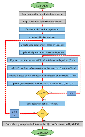
Figure 1.
Flowchart of the GMBO algorithm.
3. Simulation Study and Results
In this section, the simulation studies of the proposed GMBO in terms of providing suitable quasi-optimal solutions and solving various optimization problems are presented. The performance of the GMBO in providing a quasi-suitable solution on a set of 23 standard objective functions of different types of unimodal, high-dimensional multimodal, and fixed-dimensional multimodal functions was evaluated. Detailed information on these 23 standard objective functions is provided in Appendix A to Table A1, Table A2 and Table A3.
In order to analyze the optimization results obtained from the GMBO, these results were compared with the performance of eight other optimization algorithms, including (i) famous methods: Genetic Algorithm (GA) [20], Particle Swarm Optimization (PSO) [10], (ii) popular methods: Gravitational Search Algorithm (GSA) [16], Teaching-Learning-Based Optimization (TLBO) [21], Grey Wolf Optimizer (GWO) [11], Whale Optimization Algorithm (WOA) [12], and (iii) recently methods: Tunicate Swarm Algorithm (TSA) [13] and Marine Predators Algorithm (MPA) [14]. The experimentation was done on MATLAB (R2020a version) using a 64-bit Core i7 processor of 3.20 GHz and 16 GB of main memory. Each of the optimization algorithms was implemented twenty independent times; the optimization results are presented as the average and the standard deviation of the best solutions as “ave” and “std”, respectively.
The values used for the main controlling parameters of the comparative algorithms are specified in Table 1.

Table 1.
Parameter values for the comparative algorithms.
3.1. Evaluation Results on Unimodal Objective Functions
Seven objective functions of unimodal functions, including F1 to F7, have been selected to evaluate the performance of the GMBO in providing a quasi-optimal solution. For this purpose, the GMBO and eight other algorithms are implemented on these functions, and the optimization results are presented in Table 2. The GMBO is able to provide the basic optimal solution for the F1, F2, F3, and F6 objective functions. Additionally, the GMBO has had an acceptable performance in providing quasi-optimal solutions for the F4, F5, and F7 objective functions. The presented results in Table 2 show that the GMBO has an acceptable performance in solving the objective functions of the unimodal type and is more suitable than the eight competing optimization algorithms.
Table 2.
Optimization results of GMBO and other optimization algorithms on unimodal objective functions.
3.2. Evaluation Results on High-Dimensional Multimodal Objective Functions
Six F8 to F13 objective functions were selected to evaluate the performance of the GMBO and eight other optimization algorithms in optimizing high-dimensional multimodal functions. The optimization results of these objective functions are presented in Table 3. Based on this table, the GMBO is able to provide the basic optimal solution for the F9 and F11 objective functions. The GMBO generates the best quasi-optimal solutions for F10 and F12 objective functions. For the F13 objective function, the GSA is the best optimizer, and the GMBO is the second-best optimizer. The optimization results show that the GMBO obtains very competitive results in the majority of high-dimensional multimodal objective functions.
Table 3.
Optimization results of the GMBO and other optimization algorithms on high-dimensional test objective functions.
3.3. Evaluation Results on Fixed-Dimensional Multimodal Objective Functions
Ten objective functions of fixed-dimensional multimodal functions, including F14 to F23, were selected to evaluate the performance of the GMBO in providing quasi-optimal solutions. The results of the implementation of the GMBO and eight other optimization algorithms on this type of objective function are presented in Table 4. Based on this table, the GMBO is able to provide the basic optimal solution for the F14, F17, F18, F19, F20, F21, F22, and F23 objective functions. The GMBO for the F15 and F16 objective functions also provides quasi-optimal solutions that are very close to the global optimal solutions. The simulation results show that the GMBO provides more acceptable and competitive performance in solving this type of optimization problem.
Table 4.
Optimization results of the GMBO and other optimization algorithms on fixed-dimensional objective functions.
Table 2, Table 3 and Table 4 present the optimization results of the F1 to F23 objective functions using the GMBO and eight other compared optimization algorithms. In order to further analyze and visually compare the performance of the optimization algorithms, a boxplot of results for each algorithm and objective function is shown in Figure 2.
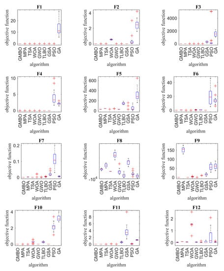
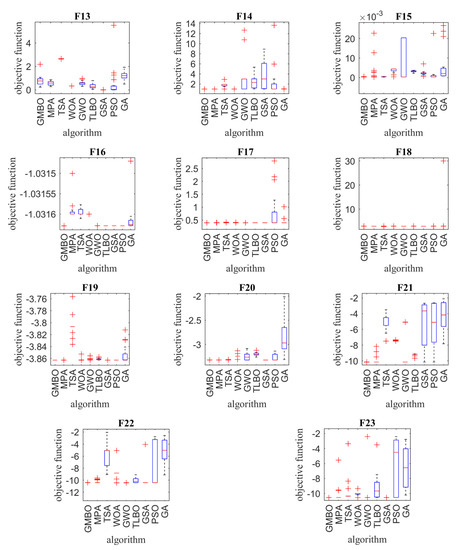
Figure 2.
Boxplot of composition objective function results for different optimization algorithms.
3.4. Statistical Analysis
This section provides a statistical analysis of the performance of the GMBO and other optimization algorithms in optimizing the mentioned objective functions. Although presenting the optimization results as the average and standard deviation of the best solutions provides valuable information on the performance of the optimization algorithms, statistical analysis is important to ensure the superiority of the proposed GMBO algorithm and the nonrandomness of this superiority. Therefore, in this study, the Wilcoxon rank-sum test, which is a nonparametric statistical test, was applied to determine the significance of the results. The Wilcoxon rank-sum test was applied to specify whether the results obtained by the proposed GMBO were different from the other eight optimization algorithms in a statistically significant way.
A p-value specifies whether the given algorithm is statistically significant or not. If the p-value of the given algorithm is less than 0.05, then the corresponding algorithm is statistically significant. The results of the analysis using the Wilcoxon rank-sum test for the objective functions are shown in Table 5. It is observed from Table 5 that the GMBO is significant superiority to the other competitor algorithms based on the p-values, which are less than 0.05.
Table 5.
Obtained results from the Wilcoxon test (p ≥ 0.05).
3.5. Sensitivity Analysis
In this section, the sensitivity of the proposed GMBO algorithm to the two parameters of the number of population members and the maximum number of iterations is analyzed.
In order to analyze the sensitivity of the proposed algorithm to the number of population members parameter, the GMBO was run independently on all 23 objective functions for the different populations with the number of 20, 30, 50, and 80 members. The results of this simulation for different numbers of population members are presented in Table 6. It is analyzed from Table 6 that for the proposed GMBO, the value of objective function decreases when the number of search agents increases. Convergence curves of GMBO for the sensitivity analysis of the number of population members are shown in Figure 3.
Table 6.
Results of algorithm sensitivity analysis of the number of population members.
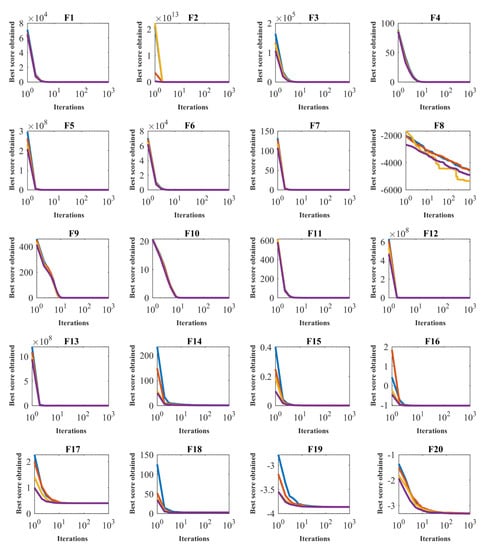
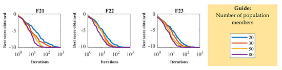
Figure 3.
Sensitivity analysis of the GMBO for the number of population members.
In order to analyze the sensitivity of the proposed GMBO algorithm to the maximum number of iterations parameter, the GMBO was run independently on all 23 objective functions for the maximum number of iterations of 100, 500, 800, and 1000. The performance of the proposed GMBO algorithm, as affected by the different maximum numbers of iterations, is presented in Table 7. The results show that GMBO converges towards the optimal solution when the maximum number of iterations is increased. Convergence curves of the GMBO for the sensitivity analysis of the maximum number of iterations are shown in Figure 4.
Table 7.
Results of algorithm sensitivity analysis of the maximum number of iterations.
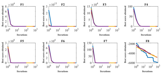
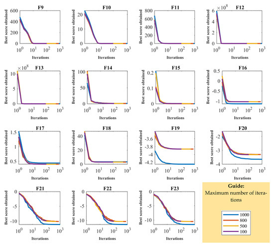
Figure 4.
Sensitivity analysis of the GMBO for the maximum number of iterations.
4. Discussion
Population-based optimization algorithms have been developed with the aim of providing a suitable quasi-optimal solution that is close to the global optimal solution. Exploitation power and exploration power are two important indicators in evaluating the performance of optimization algorithms.
Exploitation power demonstrates the ability of an optimization algorithm to provide a quasi-optimal solution to an optimization problem. In fact, based on the definition of exploitation power, an algorithm must be able to provide a quasi-optimal solution to an optimization problem after complete implementation and at the end of iterations. This indicator is especially evident in optimization problems that have only one basic optimal solution. The F1 to F7 objective functions, which are unimodal functions, have only one basic optimal solution and are, therefore, suitable for analyzing the exploitation power of optimization algorithms. The performance results of the GMBO and eight other optimization algorithms for optimizing these objective functions are presented in Table 2. These results show that the GMBO has high exploitation power and is able to provide the basic optimal solution to the problem for objective functions F1, F2, F3, F4, and F6. The GMBO also provides an acceptable quasi-optimal solution for the F5 and F7 objective functions.
Exploratory power demonstrates the ability of an optimization algorithm to accurately scan the search space of an optimization problem. According to the definition of exploratory power, an optimization algorithm should be able to explore different areas of the problem search space during implementation and successive iterations. The exploration index is especially important for optimization problems that have several local optimal solutions in addition to the basic optimal solution. High-dimensional multimodal objective functions, including F8 to F13, and fixed-dimensional multimodal objective functions, including F14 to F23, are functions that have several local optimal solutions in addition to the basic optimal solution and are, therefore, suitable for analyzing the exploration power of optimization algorithms. The optimization results of these objective functions are presented using the GMBO and eight other optimization algorithms in Table 3 and Table 4. The results show the high exploration power of the optimization algorithm in solving optimization problems with several local optimal solutions. Therefore, the GMBO is able to scan different areas of the search space well and pass through the optimal local areas with its high exploration power.
The results of the statistical analysis obtained from the Wilcoxon rank test presented in Table 5 ensure that the superiority of the GMBO over other algorithms, as well as its acceptable exploitation and exploration power, is not random.
5. Real-Life Application
In this section, the performance of the GMBO in solving problems in real-life applications is evaluated. For this purpose, the GMBO is implemented in an optimization problem, namely, pressure vessel design.
The mathematical model of this problem was adapted from [22]. Figure 5 shows the schematic view of the pressure vessel problem. Table 8 and Table 9 report the performance of the GMBO and other algorithms. The GMBO provides an optimal solution at (0.778201, 0.384739, 40.320910, 200.00000), with a corresponding objective function value of 5886.0424. Figure 6 presents the convergence analysis of the GMBO for the pressure vessel design optimization problem.
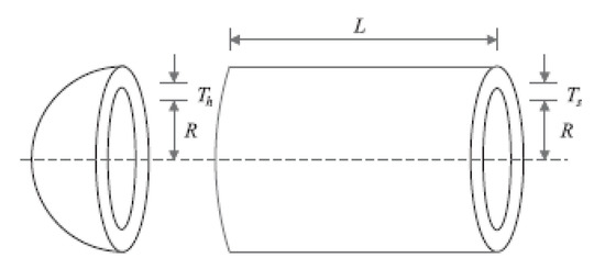
Figure 5.
Schematic view of the pressure vessel problem.
Table 8.
Comparison results for the pressure vessel design problem.
Table 9.
Statistical results for the pressure vessel design problem.
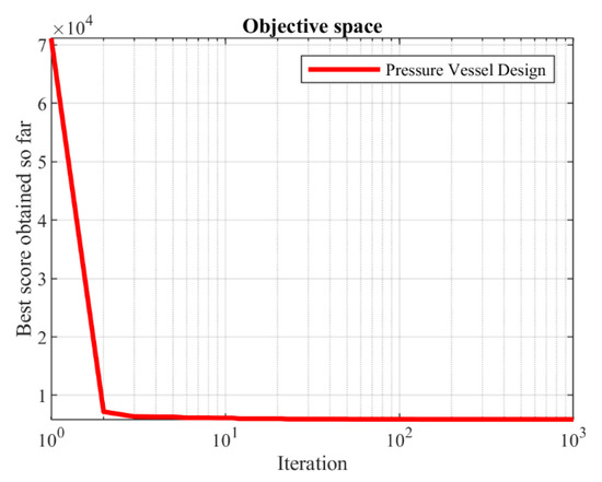
Figure 6.
Convergence analysis of the GMBO for the pressure vessel design optimization problem.
6. Conclusions and Future Works
Optimization algorithms have a special application in solving optimization problems. In this study, a new optimization algorithm called the Group Mean-Based Optimizer (GMBO) is presented to be used in solving optimization problems in various sciences. The proposed GMBO algorithm is based on the more effective use of the population members’ information by creating two new composite members by averaging two selected groups of good and bad members in updating the algorithm population. The various steps of the GMBO have been described and then modeled mathematically to apply to solving optimization problems. The performance of the GMBO in optimization was evaluated on a set of 23 standard objective functions of unimodal, high-dimensional multimodal, and fixed-dimensional multimodal types. The results of the optimization of unimodal objective functions, including F1 to F7, showed the high power of the proposed GMBO in the exploitation index. Additionally, multimodel objective functions, including two groups of F8 to F13 and F14 to F23, showed that the GMBO has a good exploration index in solving optimization problems that also have several local optimal solutions. The optimization results obtained from the GMBO were compared with eight other optimization algorithms, including the Marine Predators Algorithm (MPA), the Tunicate Swarm Algorithm (TSA), the Whale Optimization Algorithm (WOA), the Grey Wolf Optimizer (GWO), Teaching-Learning-Based Optimization (TLBO), the Gravitational Search Algorithm (GSA), Particle Swarm Optimization (PSO), and the Genetic Algorithm (GA). The optimization results show that the proposed GMBO algorithm has an acceptable ability to solve various optimization problems and is much more competitive than other algorithms. In addition, the efficiency and effectiveness of the GMBO were also demonstrated by applying it to an engineering design problem, namely, pressure vessel design. From the experimental results, it can be concluded that the GMBO is applicable to real-life studies of problems with unknown search spaces.
We propose several perspectives and ideas for future works and studies. The design of a binary version and a multiobjective version of the GMBO is an interesting potential topic for future investigations. Apart from this, applying the GMBO to real-life optimization problems and various other optimization problems can be considered significant contributions as well.
The important issue of all population-based optimization algorithms is that since population-based optimization algorithms provide a quasi-optimal solution to an optimization problem based on random search space searches, this solution may be different from the global optimal solution. Therefore, although the proposed GMBO in this paper has performed well in optimizing optimization problems, it is still possible to introduce new optimization algorithms that can provide more appropriate quasi-optimal solutions that are closer to global optimization.
Author Contributions
Conceptualization, Š.H. and M.D.; methodology, Z.M.; software, Š.H.; validation, M.D., Z.M., and Š.H.; formal analysis, Z.M.; investigation, M.D.; resources, Š.H.; data curation, Z.M.; writing—original draft preparation, M.D.; writing—review and editing, Š.H.; visualization, Z.M.; supervision, M.D.; project administration, M.D.; funding acquisition, Š.H. All authors have read and agreed to the published version of the manuscript.
Funding
The research was supported by the Project of Specific Research, PrF UHK No. 2101/2021.
Institutional Review Board Statement
Not applicable.
Informed Consent Statement
Informed consent was obtained from all subjects involved in the study.
Data Availability Statement
The authors declare to honor the Principles of Transparency and Best Practice in Scholarly Publishing about Data.
Conflicts of Interest
The authors declare no conflict of interest.
Appendix A
Table A1.
Unimodal test functions.
Table A1.
Unimodal test functions.
| Objective Function | Range | Dimensions | Fmin |
|---|---|---|---|
| 30 | 0 | ||
| 30 | 0 | ||
| 30 | 0 | ||
| 30 | 0 | ||
| 30 | 0 | ||
| 30 | 0 | ||
| 30 | 0 |
Table A2.
High-dimensional multimodal test functions.
Table A2.
High-dimensional multimodal test functions.
| Objective Function | Range | Dimensions | Fmin |
|---|---|---|---|
| 30 | −12569 | ||
| 30 | 0 | ||
| 30 | 0 | ||
| 30 | 0 | ||
| 30 | 0 | ||
| 30 | 0 |
Table A3.
Fixed-dimensional multimodal test functions.
Table A3.
Fixed-dimensional multimodal test functions.
| Objective Function | Range | Dimensions | Fmin |
|---|---|---|---|
| 2 | 0.998 | ||
| 4 | 0.00030 | ||
| 2 | −1.0316 | ||
| 2 | 0.398 | ||
| 2 | 3 | ||
| 3 | −3.86 | ||
| 6 | −3.22 | ||
| 4 | −10.1532 | ||
| 4 | −10.4029 | ||
| 4 | −10.5364 |
References
- Dhiman, G. SSC: A hybrid nature-inspired meta-heuristic optimization algorithm for engineering applications. Knowl. Based Syst. 2021, 222, 106926. [Google Scholar] [CrossRef]
- Dhiman, G.; Kaur, A. STOA: A bio-inspired based optimization algorithm for industrial engineering problems. Eng. Appl. Artif. Intell. 2019, 82, 148–174. [Google Scholar] [CrossRef]
- Li, S.; Chen, H.; Wang, M.; Heidari, A.A.; Mirjalili, S. Slime mould algorithm: A new method for stochastic optimization. Future Gener. Comput. Syst. 2020, 111, 300–323. [Google Scholar] [CrossRef]
- Dorigo, M.; Stützle, T. Ant colony optimization: Overview and recent advances. In Handbook of Metaheuristi; Springer International Publishing: Cham, Switzerland, 2019; pp. 311–351. [Google Scholar]
- Dehghani, M.; Montazeri, Z.; Dehghani, A.; Seifi, A. Spring Search Algorithm: A new meta-heuristic optimization algorithm inspired by Hooke’s law. In 2017 IEEE 4th International Conference on Knowledge-Based Engineering and Innovation (KBEI); IEEE: Tehran, Iran, 2017; pp. 210–214. [Google Scholar]
- Dehghani, M.; Montazeri, Z.; Givi, H.; Guerrero, J.M.; Dhiman, G. Darts game optimizer: A new optimization technique based on darts game. Int. J. Intell. Eng. Syst 2020, 13, 286–294. [Google Scholar] [CrossRef]
- Gaina, R.D.; Devlin, S.; Lucas, S.M.; Perez, D. Rolling horizon evolutionary algorithms for general video game playing. IEEE Trans. Games 2021. [Google Scholar] [CrossRef]
- Niccolai, A.; Grimaccia, F.; Mussetta, M.; Gandelli, A.; Zich, R. Social network optimization for WSN routing: Analysis on problem codification techniques. Mathematics 2020, 8, 583. [Google Scholar] [CrossRef]
- Roy, K.; Ting, T.C.H.; Lau, H.H.; Lim, J.B. Nonlinear behaviour of back-to-back gapped built-up cold-formed steel channel sections under compression. J. Constr. Steel Res. 2018, 147, 257–276. [Google Scholar] [CrossRef]
- Kennedy, J.; Eberhart, R. Particle swarm optimization. In Proceedings of the IEEE International Conference on Neural Networks, Perth, Australia, 27 November–1 December 1995; IEEE Service Center: Piscataway, NJ, USA, 1942; p. 1948. [Google Scholar]
- Mirjalili, S.; Mirjalili, S.M.; Lewis, A. Grey wolf optimizer. Adv. Eng. Softw. 2014, 69, 46–61. [Google Scholar] [CrossRef]
- Mirjalili, S.; Lewis, A. The whale optimization algorithm. Adv. Eng. Softw. 2016, 95, 51–67. [Google Scholar] [CrossRef]
- Kaur, S.; Awasthi, L.K.; Sangal, A.; Dhiman, G. Tunicate swarm algorithm: A new bio-inspired based metaheuristic paradigm for global optimization. Eng. Appl. Artif. Intell. 2020, 90, 103541. [Google Scholar] [CrossRef]
- Faramarzi, A.; Heidarinejad, M.; Mirjalili, S.; Gandomi, A.H. Marine Predators Algorithm: A nature-inspired metaheuristic. Expert Syst. Appl. 2020, 152, 113377. [Google Scholar] [CrossRef]
- Van Laarhoven, P.J.; Aarts, E.H. Simulated annealing. In Simulated Annealing: Theory and Applications; Springer: Berlin/Heidelberg, Germany, 1987; pp. 7–15. [Google Scholar]
- Rashedi, E.; Nezamabadi-Pour, H.; Saryazdi, S. GSA: A gravitational search algorithm. Inf. Sci. 2009, 179, 2232–2248. [Google Scholar] [CrossRef]
- Dehghani, M.; Samet, H. Momentum search algorithm: A new meta-heuristic optimization algorithm inspired by momentum conservation law. SN Appl. Sci. 2020, 2, 1–15. [Google Scholar] [CrossRef]
- Dehghani, M.; Mardaneh, M.; Guerrero, J.M.; Malik, O.; Kumar, V. Football game based optimization: An application to solve energy commitment problem. Int. J. Intell. Eng. Syst. 2020, 13, 514–523. [Google Scholar] [CrossRef]
- Dehghani, M.; Montazeri, Z.; Saremi, S.; Dehghani, A.; Malik, O.P.; Al-Haddad, K.; Guerrero, J.M. HOGO: Hide Objects Game Optimization. Int. J. Intell. Eng. Syst. 2020, 13, 216–225. [Google Scholar] [CrossRef]
- Bose, A.; Biswas, T.; Kuila, P. A novel genetic algorithm based scheduling for multi-core systems. In Smart Innovations in Communication and Computational Sciences; Springer: Berlin/Heidelberg, Germany, 2019; pp. 45–54. [Google Scholar]
- Rao, R.V.; Savsani, V.J.; Vakharia, D. Teaching–learning-based optimization: A novel method for constrained mechanical design optimization problems. Comput. Aided Des. 2011, 43, 303–315. [Google Scholar] [CrossRef]
- Kannan, B.; Kramer, S.N. An augmented Lagrange multiplier based method for mixed integer discrete continuous optimization and its applications to mechanical design. J. Mech. Des. 1994, 116, 405–411. [Google Scholar] [CrossRef]
Publisher’s Note: MDPI stays neutral with regard to jurisdictional claims in published maps and institutional affiliations. |
© 2021 by the authors. Licensee MDPI, Basel, Switzerland. This article is an open access article distributed under the terms and conditions of the Creative Commons Attribution (CC BY) license (https://creativecommons.org/licenses/by/4.0/).