Article

Probabilistic Non-Negative Matrix Factorization with Binary Components

1
College of Computer Science, Chongqing University, Chongqing 400044, China
2
National Center for Applied Mathematics in Chongqing, Chongqing Normal University, Chongqing 400044, China
3
Zhuhai UM Science & Technology Research Institute, Zhuhai 519000, China
*
Author to whom correspondence should be addressed.
Mathematics 2021, 9(11), 1189; https://doi.org/10.3390/math9111189
Submission received: 19 April 2021 / Revised: 19 May 2021 / Accepted: 20 May 2021 / Published: 24 May 2021
(This article belongs to the Section Mathematics and Computer Science)

Abstract

:
Non-negative matrix factorization is used to find a basic matrix and a weight matrix to approximate the non-negative matrix. It has proven to be a powerful low-rank decomposition technique for non-negative multivariate data. However, its performance largely depends on the assumption of a fixed number of features. This work proposes a new probabilistic non-negative matrix factorization which factorizes a non-negative matrix into a low-rank factor matrix with 0 , 1 constraints and a non-negative weight matrix. In order to automatically learn the potential binary features and feature number, a deterministic Indian buffet process variational inference is introduced to obtain the binary factor matrix. Further, the weight matrix is set to satisfy the exponential prior. To obtain the real posterior distribution of the two factor matrices, a variational Bayesian exponential Gaussian inference model is established. The comparative experiments on the synthetic and real-world datasets show the efficacy of the proposed method.

1. Introduction

Non-negative matrix factorization (NMF) is an important nonlinear technique to find purely additive, parts-based representations of non-negative multivariate data [1]. It aims to reveal the latent structure or pattern in the data. Compared with the classical low-rank matrix factorization methods, such as the singular value decomposition and principal component analysis, NMF has turned out to be a powerful tool in data-mining analysis because of its stronger explanatory properties (parts constitute the whole) and rationality (decomposing factors must be non-negative in some real scenarios). For example, image information can be compressed and summarized into a combination of some features [2], and some feature words can be learned from the document to represent the document for clustering tasks [3]. This original information is generally stored in the computer as a data matrix, which is decomposed by NMF into the product of a basis factor matrix and a weight.
Most research on the NMF algorithm is based on the specific expected characteristics to impose other restrictions except negativity on the factorization factor matrix [4,5,6]. Although these works have made some achievements, some significant problems remain to be solved, such as the way to construct efficient algorithm to avoid complex iterative calculation, and the initialization problem which greatly weaken the flexibility of the model due to its unknowability. Wild et al. [7] proposed that the use of a structured initial value can improve the efficiency of the NMF algorithm at the cost of converging to a poor local solution.
The probability non-negative matrix factorization from statistical view may be enlightening. Bayesian NMF is the NMF model with KL penalty that was extended to the Bayesian setting [8]. Using the Bayesian nonparametric model of infinite dimensional parameter space, the number of features is determined as a random quantity in the process of posterior inference. Indian buffet process (IBP) is a classical latent feature model. This method generates a prior of a binary matrix, which has finite dimensional rows (number of objects) and infinite dimensional columns (number of features) [9]. The real latent finite element information can be obtained completely by the posterior inference with IBP. Many studies have proposed the application of IBP in NMF. For example, Yang et al. projected a non-negative binary matrix tri-factorization model that better reveals the underlying structure between samples and features, including two binary matrices and a weight matrix [10].
In this work, we come up with a new special probabilistic non-negative matrix factorization which requires the basis matrix Z atisfies 0 , 1 constraints and the weighted matrix A is non-negative. This is clearer and more intuitive than the definition of tri-factorization proposed in [10]. For the binary matrix Z , the IBP is introduced to solve, and we assume that the weight matrix A obeys the exponential distribution under the non-negative constraint. In addition, based on synthetic dataset and real-world datasets, we compare our approach with benchmark methods to verify its flexibility and effectiveness. Main contributions are following three aspects:
(1)
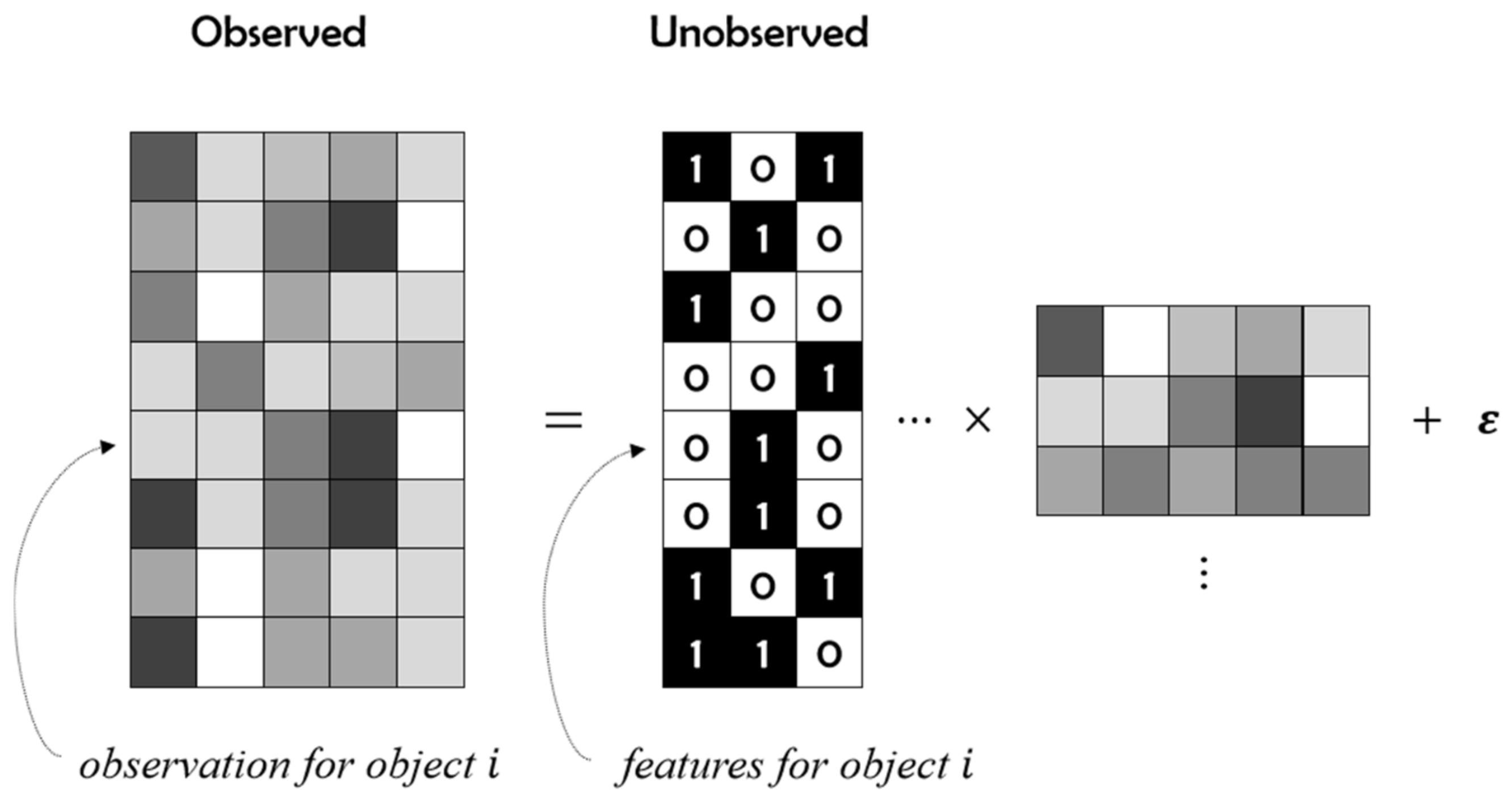
We present a pNMF with single binary component. Compared with other methods, the binary matrix can be regarded as the mapping from real object to binary codes, which is more intuitive.
(2)
IBP is applied to the pNMF and we explain its use as a prior in the variational Bayesian exponential Gaussian model. The real latent information is completely obtained by inference and the sensitivity of the model to initialization parameter setting is greatly reduced.
(3)
The experiments on the synthesized dataset and real-world datasets show the validity of the proposed method.
The rest of this paper is organized as follows: the related work is outlined in the next section. Section 3 explains the proposed method and the derivation process. Section 4 gives the empirical research results on four different types of dataset. The last section concludes the work.

2. Related Work

Recent research has inspired us to consider pNMF with single components on the basis of IBP. This section lists the literature review of NMF and IBP.

2.1. Non-Negative Matrix Factorization

NMF was firstly posed by Paatero and tapper [1], but enjoyed wide popularity due to the research results of Lee and Seung [2]. According to its definition, the factor elements after factorization must be non-negative, and simultaneously achieves nonlinear dimension reduction. Mathematically, given the non-negative matrix V , the problem is to find two factor matrices W 0 and H 0 to approximate V , so that V W H . It is also usually interpreted as V = W H + ε by researchers with blind source signal separation background [11], where ε is a noise matrix. Lee and Seung [2] also introduced two simpler algorithms whose objective functions are based on Euclid distance and Kullback–Leibler divergence (KL), respectively, and they proved the convergence of iterative rules. As an unsupervised learning method, NMF is widely used in many fields.
Many improved NMF algorithms have been advocated in recent years. Hoyer et al. [12] combined sparse penalty term with NMF to construct the sparse NMF model, in which parameters were solved by the gradient projection method and the EM algorithm. Wang et al. [13] combined Fisher’s discriminant criterion with the objective function of non-negative matrix factorization to extract local features. Lin et al. [14] brought forth an optimization algorithm of NMF based on projection gradient method, which refined the convergence rate of factorization. Liu et al. [6] found a restrictive NMF algorithm under semi-supervised learning that effectively combined the category information. Guillamet et al. [15] pointed out a weighted NMF algorithm to solve the image classification problem by better representation ability of local features.
For many NMF methods, the rank needs to be determined in advance, and its value was adjusted and searched through trial and error. Hinrich et al. [16] mentioned a probabilistic sparse NMF model that extends the variational Bayesian NMF and explicitly considers sparsity. Mohammadiha et al. [17] developed a hidden Markov model whose output density function is a gamma distribution. This model was reformulated as a probabilistic NMF, and it can capture the time dependence internally. To derive the maximum a posterior (MAP) of the non-negative factors, Shterenberg et al. [18] extended the NMF deterministic framework to the probabilistic such that the original data are no longer deterministic, which is considered to be a sample drawn from a multinomial distribution.

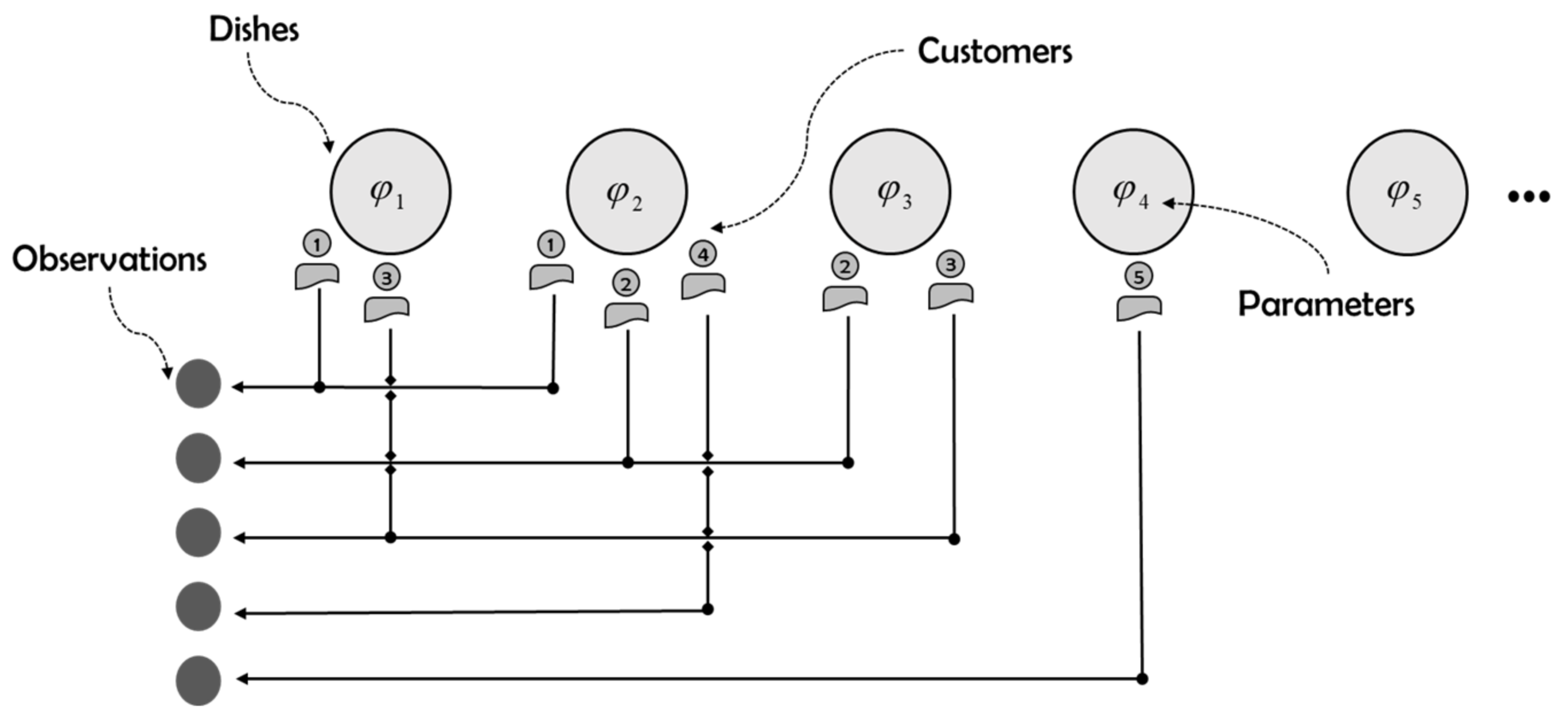
2.2. Indian Buffet Process

Griffiths et al. [9] proposed the IBP in 2005. They defined the probability distribution over equivalence classes of a binary matrix with a finite number of rows and an unbounded number of columns, and illustrated the use of it as a prior in an infinite binary linear–Gaussian model. At the same time, they have proved that this distribution as a prior is suitable for probabilistic models that use potentially infinite feature arrays to represent objects [19]. Many studies have been extended on the basis of IBP to generate more general distribution categories.
Ghahramani et al. [20] introduced a two-parameter generalization of the IBP that focused on separating the coupling relationship between the total number of features and the distribution on the feature number of each object. The et al. [21] analyzed the stick-breaking construction of IBP and developed a slice sampler with higher efficiency and easier application. Thibaux and Jordan [22] demonstrated the exchangeable distribution produced by IBP corresponds to the use of a latent measure based on the beta process. Gael et al. [23] rendered a strategy for modifying the IBP to capture the dependency which can arise as the observations being generated in a specific sequence. Miller et al. [24] used the phylogenetic IBP to seek a dependency that is taken as the result of known degrees of relatedness among observations.
The significance of IBP is to produce a distribution of infinite sparse binary matrix, which can be used to define many new non-parametric Bayesian models with different likelihood functions. Miller et al. [25] defined a class of non-parametric latent feature models that can be used for link prediction. Meeds et al. [26] presented a model of dyadic data based on the two-parameter IBP and developed some novel Metropolis-Hasting proposals for inference. Wood et al. [27] adopted a non-parametric Bayesian approach based on the IBP to model the structure graphs with many hidden causes. Navarro et al. [28] proposed a non-parametric Bayesian model for inferring features from similarity judgements.

3. The Proposed Methods

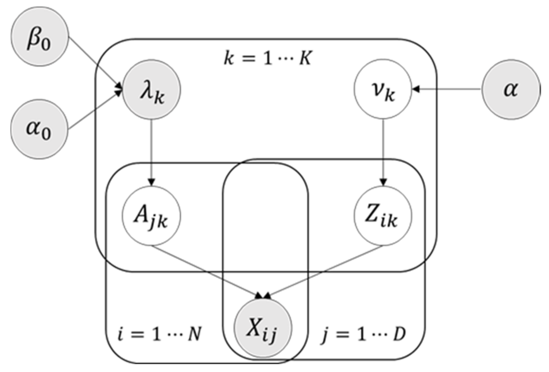
3.1. Model Framework

Given a non-negative matrix X N × D , the product of two non-negative factor matrices Z and A is expected to be as close to X as possible. Our data model is shown in Figure 1.
Where Z is a binary matrix of N × K dimension, and A is a non-negative weight matrix of K × D dimension. In this model, X follows the Gaussian conditional distribution:
X Z A   s . t .   Z { 0 , 1 } N × K a n d   A + K × D .
X n N o r m a l Z n A , σ n 2 ,   f o r   n 1 , , N .
According to Bayesian rule:
p ( Z , A | X ) p ( X | Z , A ) p A m o d e l   s p e c i f i c × p Z p r i o r   o n   b i n a r y   m a t r i x .
It can be seen that each column in Z corresponds to the existence of a latent feature, and all elements of Z are non-negative due to the 0 , 1 constraints. p Z is just the prior probability function defined by IBP on the binary matrix Z in (1). For A , we need a prior to express rules about its value, so we assumed that A obeys the exponential distribution to meet the non-negative limitation. Thus, each element of A obeys the exponential distribution [8].
Therefore, the defined model can be considered as an exponential Gaussian model, and the prior representation of these two matrices is:
A j k ε A j k | λ k ,       λ k G λ k | α 0 , β 0 ,     z n k B e r n o u l l i π k ,   s . t .   k 1 , , , j 1 , , D ,   n 1 , , N .
In accordance with the automatic association determination algorithm proposed by Thomas et al. [29], the parameter λ is set using gamma prior, which helps the automatic selection of the model. The whole factor k is either “activated” or “off”, and only a few effective factors are set to 0 based on the magnitude of λ . Figure 2 indicates the graph structure of the exponential Gaussian model.
According to (3), the goal of our model is to obtain the true posterior distribution l n ( p ( Z , A | X , σ n 2 , α , λ ) ) of factor matrices. It is very difficult to solve this problem with conventional methods, but the variational approximation algorithm is likely to be an effective method. Many studies have revealed that this algorithm simplifies inference process and guarantees accuracy to a certain extent.
Like Gibbs sampling, the mean field variational inference is a common approximate Bayesian inference method, which is to simplify the calculation when the introduced variational distribution q θ is as close to the real distribution p ( θ | X ) as possible. The theory assumes that the variational distribution q can be completely decomposed as q θ = i q θ i , and all variables are calculated independently in the process of posteriori inference. It has been proved in [30] that the optimal distribution q * θ i of the ith parameter can be expressed as follows:
l o g   q * θ i = E q θ i l o g   p θ , X + C .
where C is a constant. The objective function is usually to maximize the lower bound of evidence (ELBO) or minimize the KL divergence as much as possible, and it is essential to choose a suitable approximate distribution q for solving the variational problems.
On the basis of the model framework, our work is mainly to find the best approximate distribution of two factor matrices that are consistent with the constraints.

3.2. The Solution of Weighted Matrix A

For the weight matrix A , the exponential distribution is used as a prior in the model to limit its non-negativity. According to Bayes’ rule, the posterior of A is approximately a truncated normal distribution if Z is fixed. The formula is as follows:
q * A j k e x p E q θ A j k l o g   p X | θ + l o g   p θ e x p E q θ A j k i Ω j l o g τ 2 π e x p τ 2 ( X i j Z i A j ) 2 + l o g λ k   e x p { λ k A j k } × u x e x p E q θ A j k i Ω j τ 2 ( X i j Z i A j ) 2 λ k A j k × u x e x p E q θ A j k τ 2 i Ω j Z i k 2 A j k 2 2 Z i k A j k X i j k k Z i k A j k A j k λ k ˜ × u x e x p A j k   λ k ˜ + τ ˜ i Ω j X i j k k Z i k ˜ A j k ˜ Z i k ˜ A j k 2 2 τ ˜ i Ω j Z i k 2 ˜ × u x e x p τ j k 2 A j k μ j k 2 × u x T N ( A j k | μ j k , τ j k ) .
Here,
T N x | μ , τ = τ 2 π e x p { τ 2 ( x μ ) 2 } 1 Φ μ τ           i f   x 0                                     0                                       i f   x < 0 ,
where A j k represents all elements in the matrix A j k except the k t h column, and it can be seen that the posterior probabilities of non-positive elements are all set to 0. This process is not a strict optimization of A , which may cause some errors in the final reconstruction results.
According to the derivation process of (6), the mean and variance of the true posterior q * A j k can be obtained as follows:
τ j k = τ ˜ i Ω j Z i k 2 ˜ ,     μ j k = 1 τ j k λ k ˜ + τ ˜ i Ω j X i j k k Z i k ˜ A j k ˜ Z i k ˜ .
It can be found that the smaller the mean (negative), the larger the variance. The truncated distribution is closest to the exponential distribution when the expected scale parameter is μ τ . In order to prevent the calculation of mean and variance effectively from being invalidated by numerical errors, it is necessary to restrict μ . The setting of parameter λ is also an important factor affecting the lower bound of X . We assume that it satisfies the following distribution and update the relevant parameters:
q A j k = T N A j k ; μ j k , τ j k ,       q λ k = G λ k ; α k * , β k * , α k * = α 0 + D ,   β k * = β 0 + j = 1 D A j k ˜ .

3.3. The Solution of Binary Matrix Z

The generation process of IBP is similar to many Indian cafeterias in London. Endless plates line up, and customers enter one by one, choosing food from left to right. If selected by a customer, this dish is marked as “1”, otherwise “0”. The number of dishes selected by each customer satisfies the Poisson distribution [9]. The process is shown in Figure 3.
As shown in Figure 3, the binary sequence representing the choice of the third customer can be expressed as 1 ,   0 ,   1 ,   0 ,   0 , . By connecting N pieces of such sequence vertically, IBP generates a priori of a binary matrix with finite number of rows (number of data) and infinite number of columns (number of latent features) to define many new non-parametric Bayesian models with different likelihood functions. Combined with the analysis of the model framework, IBP is used to approximate the binary basis matrix Z . In order to facilitate the process of variational derivation, the stick breaking construction based on the research of The et al. [16] is introduced as follows:
v j B e t a α , 1 ,     π k = j = 1 k v j ,       z n k B e r n o u l l i π k .
where v j   is the variable, α is a parameter of the beta distribution and π k is the truncated weight of column k . The basis matrix Z in our model adopts the approximate form similar to the infinite variational approach of linear Gaussian model proposed by Doshi et al. [12]:
q v n k z n k = B e r n o u l l i z n k ; v n k ,     q τ k v k = B e t a v k ; τ k 1 , τ k 2 .
To facilitate calculation, the π is replaced by v . The derivation of v and its parameters are given in [12]. We will present this information in detail in the following derivation.

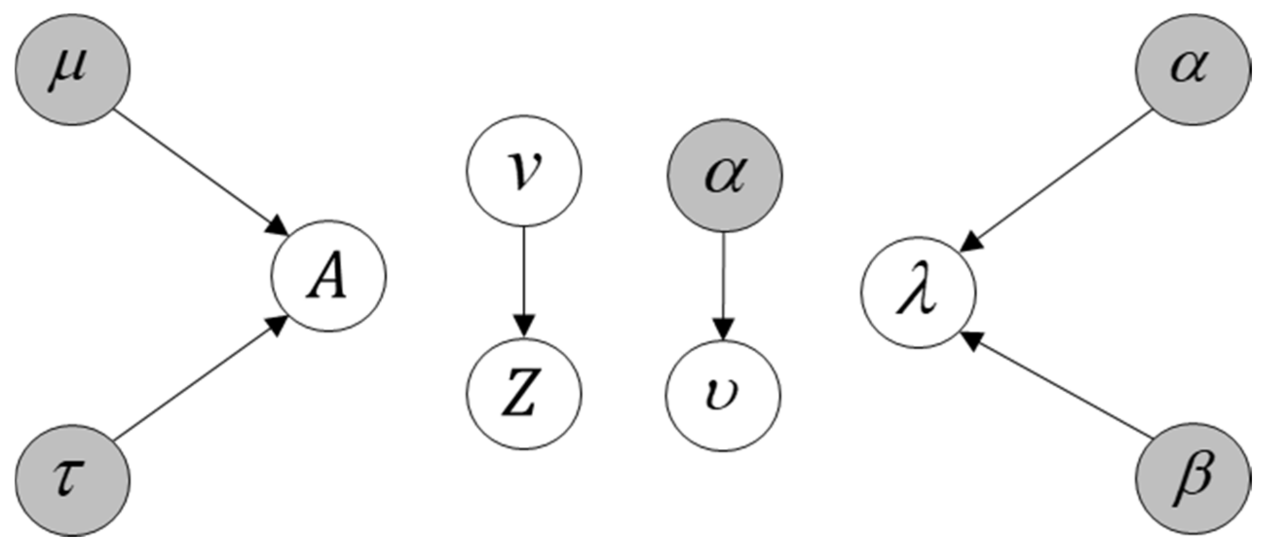
3.4. Variational Inference Process

Based on the above analysis, the variation distribution of our model is shown in Figure 4.
Since it is difficult to take the real expectation of the log joint likelihood l o g   p ( X | θ ) , this paper gives its lower bound through reasoning. The variational objective function of our model is as follows:
l o g   p ( X | θ ) k = 1 K E v [ l o g   p ( v k | α ) ] + k = 1 K n = 1 N E v , Z [ l o g   p ( Z n k | v ) ] + k = 1 K E λ [ l o g   p ( λ k | α 0 , β 0 ) ] + k = 1 K j = 1 D E λ , A [ l o g   p ( A j k | λ j k ) ] + n = 1 N E Z , A [ l o g   p ( X n | Z , A , σ n 2 ) ] + H q ,
where θ = α , α 0 , β 0 , σ n 2 is the parameter. From (12), It can be found from (12) that except the second term, all items are calculated by exponential distribution family, and their expected value derivation can refer to the study of Doshi et al. [12]. The E λ is:
k = 1 K E λ l o g   p λ k | α 0 , β 0 = α 0   l o g   β 0 l n   Γ α 0 + α 0 1 k = 1 K ψ α k + β 0 k = 1 K α k β k .
According to the research results of Chopin and Mazet [31,32], we can draw the truncated distribution formula and simulate the Gaussian distribution defined on the finite interval a , b . The semi finite interval can still be considered by setting b = + . The principle of this method is to divide the interval into the same area and use a properly distributed accept–reject algorithm. Since the A j k is a truncated normal distribution, the E λ , A is:
E λ , A l o g   p A k | λ k = E λ , A l o g ( λ k · e x p ( λ k A k ) = E λ , A l o g   λ k λ k A k ]   = l o g   λ k λ k E A k = l o g α k β k α k β k μ k + τ k · 1 2 π τ k · e x p u k 2 2 τ k / 1 2 e r f c τ k 2 · μ k .
For the lower truncated normal distribution, the expectation is as follows:
E x | x < c = μ + σ 2 f c S c .
Here f x is the probability density function and S x is the complementary cumulative distribution function, and their formulas are as follows:
f x = 1 2 π σ e x p x μ 2 2 σ 2 , S x = 1 F x = 1 c d f x = 0.5 erfc x 2   .
The entropy H q in (11) is:
H q = E q l o g k = 1 K q τ k π k k = 1 K q λ k k = 1 K q μ k A k k = 1 K n = 1 N q v n k z n k = k = 1 K E π l o g   q τ k π k + k = 1 K E λ l o g   q λ k + k = 1 K E A l o g   q μ k A k + k = 1 K n = 1 N E Z l o g   q v n k z n k
where,
E π l o g   q τ k π k = l o g Γ τ k 1 Γ τ k 2 Γ τ k 1 + τ k 2 τ k 1 1 ψ τ k 1 τ k 2 1 ψ τ k 2 + τ k 1 + τ k 2 2 ψ τ k 1 + τ k 2 , E λ l o g   q λ k = l n   Γ α k * α k * 1 ψ α k * l n   β k * + α k   * , E A l o g   q μ k A k = 0.5 l o g ( 2 π e ) D τ k   , E Z l o g   q v n k z n k = 1 v n k l o g ( 1 v n k ) v n k l o g   v n k   .
The ψ · is a digamma function. According to the analysis, the derivation formula of the final objective function of (12) is as follows:
l o g   p X | θ k = 1 K l o g   α + α 1 ψ τ k 1 ψ τ k 1 + τ k 2 + k = 1 K n = 1 N v n k m = 1 k ψ τ k 2 ψ τ k 1 + τ k 2 + 1 v n k E υ l o g 1 m = 1 k υ m + α 0 l o g   β 0 l n   Γ α 0 + α 0 1 k = 1 K ψ α k + β 0 k = 1 K α k β k + l o g α k β k α k β k μ k + τ k · 1 2 π τ k ·   e x p u k 2 2 τ k / 1 2 e r f c τ k 2 μ k + n = 1 N D 2 l o g 2 π σ n 2 + n = 1 N 1 2 σ n 2 X n X n T 2 k = 1 K v n k μ k X n T + 2 k < k v n k v n k μ k μ k T + k = 1 K v n k t r τ k + μ k μ k T + k = 1 K l o g Γ τ k 1 Γ τ k 2 Γ τ k 1 + τ k 2 τ k 1 1 ψ τ k 1 τ k 2 1 ψ τ k 2 + τ k 1 + τ k 2 2 ψ τ k 1 + τ k 2 + k = 1 K 1 2 l o g ( 2 π e ) D τ k + k = 1 K l n   Γ α k * α k * 1 ψ α k * l n β k * + α k * + k = 1 K n = 1 N v n k l o g   v n k 1 v n k l o g ( 1 v n k ) .

4. Experimental Result

The ability of the proposed method to perform matrix factorization and learn the number of latent features through the synthetic dataset is first demonstrated, and then the performance of the proposed method is verified by comparing with the benchmark methods on real datasets, including Swimmer dataset, Cora document dataset, and CBCL face dataset. While showing the effect of the model, we list the initialization setting of the parameters in each task, which have a great impact on the quality of convergence.
The main parameters involved in the experiment include IBP parameter α , lambda parameter α 0 ,   β 0 , Gaussian parameter σ n and truncated feature number K . The optimal effect parameter will be given for reference at the end of each experiment. The algorithm experiment is carried out in the environment of Matlab2015b.

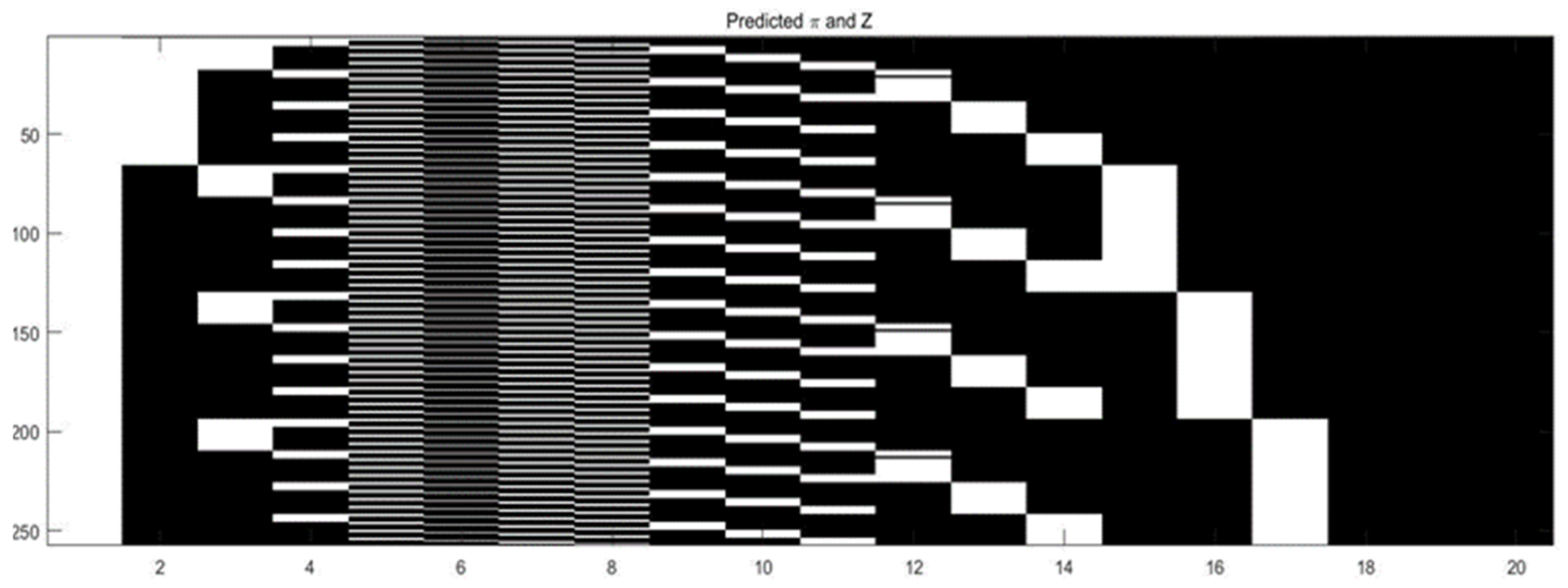
4.1. Sythetic Dataset

We apply the model to a simple composite dataset generated from known features. The dataset is simple enough, and the accuracy of graph reconstruction can reach almost 100%, and there are enough differences to resolve the qualitative features of latent feature inference. We have generated a specific 20 × 16 -dimensional non-negative matrix, some of which is shown in Figure 5.
Figure 5a shows the basis matrix Z with 20 × 4 dimension. Figure 5b shows the extracted latent features, there are four in total. The original image is sufficient to justify it. For example, the first image is made up of three feature elements in Figure 5b except for the item in the upper right corner, while the third image contains that single item.
Figure 5d shows the reconstructed image using the extracted latent features, and the comparison shows that the accuracy can reach almost 100%.
The above analysis fully proves the effectiveness of our algorithm for automatic learning of latent features. Then, the parameters are initialized as α = 1 ,   α 0 = 0.1 , β 0 = 10 , K = 6 .

4.2. Swimmer Dataset

The swimmer dataset contains all possible combinations of swimmer’s body postures (including limbs and trunk), with a total of 256 grayscale images. Figure 6 shows some samples of the dataset, depicting four simplified human figures with limbs and showing the different joints of the limbs. In this paper, the dataset is represented as a 256 × 1024 -dimensional matrix X , and each column represents a 32 × 32 -dimensional image.
The experiment is designed to observe 16 variable limb features and 1 fixed trunk feature through model learning. The trunk and limbs should be separate parts. According to our model, 17 features are accurately extracted, as shown in Figure 7.
On the contrary, most previous studies cannot successfully separate the backbone part. Since our algorithm is based on the NMF framework, the result of the basic NMF is first shown in Figure 8a. This result is derived from the research results of Gao Liang et al. in [33]. It can be seen that the eighth base image in the first line is almost identical to the sixth in the second line. The body part exists in each extracted feature, so the basic NMF method cannot independently extract the inherent or variable features of the dataset, and there is obvious overlap between the base feature values.
Figure 8b shows the result of feature extraction in [34]. It can be seen that the four basic images that have been specially labeled are all a combination of limbs and the trunk. This is contrary to common sense.
Referring to two comparative experimental methods, a series of actual factors have been “polluted” to a certain extent. The results show that the proposed method has good data representation and feature recognition ability.
In addition, Figure 9 shows the basis matrix Z . The parameters are initialized as α = 1 ,   σ n = 0.1 ,   α 0 = 1 ,   β 0 = 1 ,   K = 20 .

4.3. Document Clustering

In this subsection, we apply the proposed model to a practical task: document clustering. The Cora dataset is used for experimental data that contains 2708 papers, including 1433 unique words after removing the stop words and the words that appear less than 10 times in the literature. The labels of these documents are their research field, about 7 categories. In order to better measure the effect of clustering task, we use three evaluation indicators: Jaccard coefficient (JC), Fowlkes and Mallows (FM), and F-measurement (F1). The larger their value, the better the clustering effect is, and their formulas are as follows:
J C = a / ( a + b + c ) , F M = a / a + b a / a + c   , F 1 = 2 a 2 / 2 a 2 + a c + a b .
where a is the number of point pairs belonging to the same cluster in the benchmark results and test results, b is the number of point pairs in the same benchmark but different cluster, and c is the number of point pairs in the same cluster but different benchmark cluster.
The results of our method are compared with some parametric models, such as spectral clustering (SP), sparse NMF (SNMF), NMF, and also some Bayesian non-parametric models, which will be described in Table 1.
The benchmark comparison data are obtained from [35]. The Bivariate-Beta distribution (BB-dIBP-NMF) and Gaussian process (GP-dIBP-NMF) are proposed based on doubly IBP. Finally, in our model, 14 latent features are obtained from the dataset, others are 17 (from BB-dIBP-NMF), 22 (from GP-dIBP-NMF). It can be seen that, compared with various methods mentioned in other papers, our algorithm obtains the best clustering results with the least features. Figure 10 shows this result more visually.
The parameters are initialized as α = 20 ,   σ n = 0.1 ,   λ = 100 . And the square difference σ of spectral clustering is set to 0.2.

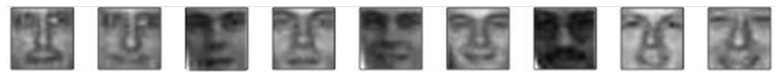
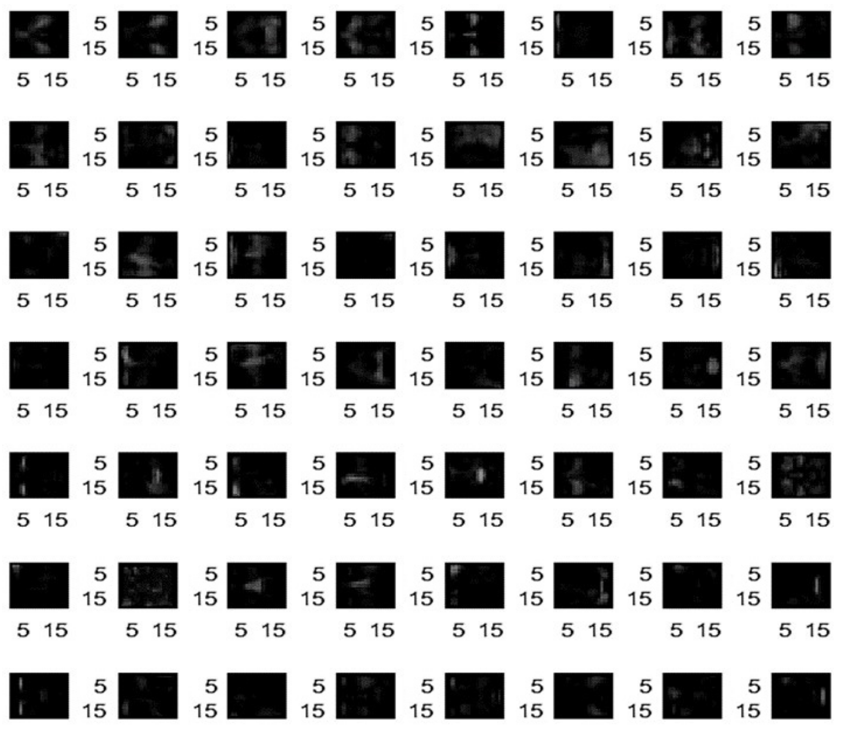
4.4. Face Feature Extraction

Not only can NMF decompose quickly and accurately, but the decomposition result has definite physical meaning. Lee and Seung [2] took face recognition as an example to decompose the face into separate parts such as nose, eyes, mouth and eyebrows. This is consistent with the intuitive visual concept of “the parts constitute the whole” in human thinking. And they compared the decomposition results of the NMF algorithm with those of common matrix factorization methods such as vector quantization (VQ) and PCA. The difference is that NMF is based on partial facial representations, while VQ and PCA are global representations. Therefore, we aim to apply the proposed model to the same face dataset (CBCL Face Database) [36] and observe whether our model can accurately extract similar local features and completely reconstruct the entire face, which is conducive to verifying the effectiveness of our model.
The CBCL Face Database contains many face and non-face images. It is widely used in the Biology and Computing Learning Center of the MIT. We use 2429 face images in the training set. Figure 11 shows some face images in this dataset.
According to the algorithm model, we extracte 51 “local” facial features from 2429 images, while 49 features are extracted by Lee and Seung [2]. Figure 12 shows facial feature extracted by our model, where white pixels represent features and the black is set as background.
Figure 13 shows the comparison between the reconstructed specific face image and the original image. By calculation, the mean square error rate of the reconstruction of the whole dataset is only 8%.
The parameters are initialized as α = 12 ,   σ n = 1 ,   α 0 = 3 ,   β 0 = 1 .

5. Conclusions

As we know, traditional NMF models need to assume the number of basis to be fixed which makes them less flexible for many applications. IBP provides a priori of an infinite binary matrix, which is usually used to infer latent features and their quantities from a set of observation data. In this paper, we propose an improved IBP based probabilistic NMF framework, which uses exponential distribution and 0 , 1 onstraints to limit the non-negativity of the weight matrix and the basis matrix. This method allows us to flexibly choose appropriate parameters as the basis to avoid the problems caused by the initial decomposition rank setting, and to automatically learn the latent features. At the same time, an exponential Gaussian model is constructed based on this framework, and the true posterior of two factor matrices is derived with the variational Bayes method. Compared with the benchmark methods, the proposed method has achieved better results on both synthetic and real datasets, and it shows higher decomposition efficiency. However, the proposed model has great computational complexity. The efficiency of execution and the reduction of model complexity may be one of the future research contents.

Author Contributions

Conceptualization, X.M. and T.Z.; methodology, X.M., J.G., and T.Z.; writing—original draft preparation, X.M. and J.G.; writing—review and editing, X.M., X.L., and J.G.; visualization, X.M. and X.L.; supervision, T.Z. and Y.T. All authors have read and agreed to the published version of the manuscript.

Funding

This work was supported in part by the National Natural Science Foundation of China (No.62076043) and the Science and Technology Research Program of Chongqing Municipal Education Commission (No. KJQN201900110).

Institutional Review Board Statement

Not applicable.

Informed Consent Statement

Not applicable.

Data Availability Statement

No data available.

Conflicts of Interest

The authors declare no conflict of interest.

References

  1. Paatero, P.; Tapper, U. Positive matrix factorization: A non-negative factor model with optimal utilization of error estimates of data values. Environmetrics 1994, 5, 111–126. [Google Scholar] [CrossRef]
  2. Lee, D.; Seung, H. Learning the parts of objects by nonnegative matrix factorization. Nature 1999, 401, 788–791. [Google Scholar] [CrossRef] [PubMed]
  3. Ramsay, J.O. Functional Data Analysis. In Encyclopedia of Statistical Sciences; Everitt, B.S., Howell, D.C., Eds.; John Wiley & Sons, Inc.: Hoboken, NJ, USA, 2004; p. 4. [Google Scholar]
  4. Bach, F.; Mairal, J.; Ponce, J. Convex sparse matrix factorizations. arXiv 2008, arXiv:0812.1869. [Google Scholar]
  5. Zafeiriou, S.; Tefas, A.; Buciu, I.; Pitas, I. Exploiting discriminant information in nonnegative matrix factorization with application to frontal face verification. IEEE Trans. Neural. Netw. Learn Syst. 2006, 17, 683–695. [Google Scholar] [CrossRef] [PubMed] [Green Version]
  6. Liu, H. Constrained nonnegative matrix factorization for image representation. IEEE Trans. Pattern Anal. Mach. Intell. 2012, 34, 1299–1311. [Google Scholar] [CrossRef]
  7. Cai, D.; He, X.; Han, J.; Huang, T.S. Graph regularized nonnegative matrix factorization for data representation. IEEE Trans. Pattern Anal. Mach. Intell. 2011, 33, 1548–1560. [Google Scholar]
  8. Schmidt, M.N.; Winther, O.; Hansen, L.K. Bayesian Non-Negative Matrix Factorization. In Independent Component Analysis and Signal Separation, Proceedings of the 8th International Conference on Independent Component Analysis and Signal Separation, Paraty, Brazil, 15 March 2009; Adali, T., Christian, J., Romano, J.M.T., Barros, A.K., Eds.; Springer: Berlin, Germany, 2009; pp. 540–547. [Google Scholar]
  9. Wild, S.; Curry, J.; Dougherty, A. Improving non-negative matrix factorizations through structured initialization. Pattern Recognit. 2004, 37, 2217–2232. [Google Scholar] [CrossRef]
  10. Yang, X.; Huang, K.; Zhang, R.; Hussain, A. Learning latent features with infinite nonnegative binary matrix trifactorization. IEEE Trans. Emerg. Top. Comput. 2018, 2, 450–463. [Google Scholar] [CrossRef] [Green Version]
  11. Zhang, Y.; Fang, Y. A NMF algorithm for blind separation of uncorrelated signals. In Proceedings of the International Conference on Wavelet Analysis and Pattern Recognition, Beijing, China, 2 November 2007; Curran Associates Inc.: New York, NY, USA, 2007; pp. 999–1003. [Google Scholar]
  12. Hoyer, P.O. Non-negative matrix factorization with sparseness constraints. J. Mach. Learn. Res. 2004, 5, 1457–1469. [Google Scholar]
  13. Jia, Y.W.Y.; Turk, C.H.M. Fisher non-negative matrix factorization for learning local features. In Proceedings of the Asian Conference on Computer Vision, Seoul, Korea, 27 January 2004; Hong, K.S., Zhang, Z.Y., Eds.; Asian Federation of Computer Vision Societies: Seoul, Korea, 2004; pp. 27–30. [Google Scholar]
  14. Lin, C.J. Projected gradient methods for nonnegative matrix factorization. Neural Comput. 2007, 19, 2756–2779. [Google Scholar] [CrossRef] [PubMed] [Green Version]
  15. Guillamet, D.; Vitria, J.; Schiele, B. Introducing a weighted non-negative matrix factorization for image classification. Pattern Recogn. Lett. 2003, 24, 2447–2454. [Google Scholar] [CrossRef]
  16. Hinrich, J.L.; Mørup, M. Probabilistic Sparse Non-Negative Matrix Factorization. In Latent Variable Analysis and Signal Separation, Proceedings of the International Conference on Latent Variable Analysis and Signal Separation, Guildford, UK, 2 July 2018; Deville, Y., Gannot, S., Mason, R., Plumbley, M., Ward, D., Eds.; Springer: Berlin, Germany, 2018; pp. 488–498. [Google Scholar]
  17. Mohammadiha, N.; Kleijn, W.B.; Leijon, A. Gamma hidden Markov model as a probabilistic nonnegative matrix factorization. In Proceedings of the 21st European Signal Processing Conference (EUSIPCO 2013), Marrakech, Morocco, 9 September 2013; IEEE: New York, NY, USA, 2013; pp. 1–5. [Google Scholar]
  18. Bayar, B.; Bouaynaya, N.; Shterenberg, R. Probabilistic non-negative matrix factorization: Theory and application to microarray data analysis. J. Bioinform. Comput. Biol. 2014, 12, 1450001. [Google Scholar] [CrossRef] [PubMed]
  19. Griffiths, T.L.; Ghahramani, Z. The Indian buffet process: An introduction and review. J. Mach. Learn. Res. 2011, 12, 1185–1224. [Google Scholar]
  20. Knowles, D.; Ghahramani, Z. Infinite Sparse Factor Analysis and Infinite Independent Components Analysis. In International Conference on Independent Component Analysis and Signal Separation, ICA’07, Proceedings of the 7th International Conference on Independent Component Analysis and Signal Separation, London, UK, 12 August 2007; Davies, M.E., James, C.J., Abdallah, S.A., Plumbley, M.D., Eds.; Springer: Berlin, Germany, 2007; pp. 381–388. [Google Scholar]
  21. Teh, Y.W.; Grür, D.; Ghahramani, Z. Stick-Breaking Construction for the Indian Buffet Process. In Artificial Intelligence and Statistics, Proceedings of the Eleventh International Conference on Artificial Intelligence and Statistic, San Juan, PR, USA, 21–24 March 2007; Meila, M., Shen, X., Eds.; PMLR: San Juan, PR, USA, 2007; pp. 556–563. [Google Scholar]
  22. Thibaux, R.; Jordan, M.I. Hierarchical Beta Processes and the Indian Buffet Process. In Artificial Intelligence and Statistics, Proceedings of the Eleventh International Conference on Artificial Intelligence and Statistic, San Juan, PR, USA, 21–24 March 2007; Meila, M., Shen, X., Eds.; PMLR: San Juan, PR, USA, 2007; pp. 564–571. [Google Scholar]
  23. Gael, J.V.; The, Y.; Ghahramani, Z. The infinite factorial hidden Markov model. In Proceedings of the 21th International Conference on Neural Information Processing Systems, Vancouver, BC, Canada, 8–10 December 2008; Koller, D., Schuurmans, D., Bengio, Y., Bottou, L., Eds.; Curran Associates Inc.: New York, NY, USA, 2008; pp. 1697–1704. [Google Scholar]
  24. Miller, K.T.; Griffiths, T.L.; Jordan, M.I. The phylogenetic Indian buffet process: A non-exchangeable nonparametric prior for latent features. In Proceedings of the 24th Conference on Uncertainty in Artificial Intelligence, Helsinki, Finland, 9–12 July 2008; Mcallester, D., Myllymaki, P., Eds.; AUAI Press: Arlington, VA, USA, 2008; pp. 403–407. [Google Scholar]
  25. Miller, K.T.; Griffiths, T.L.; Jordan, M.I. Nonparametric latent feature models for link prediction. In Proceedings of the 22nd International Conference on Neural Information Processing Systems, Vancouver, BC, Canada, 7–10 December 2009; Bengio, Y., Schuurmans, D., Lafferty, J.D., Williams, C.K.I., Culotta, A., Eds.; Curran Associates Inc.: New York, NY, USA, 2009; pp. 1276–1284. [Google Scholar]
  26. Meeds, E.; Ghahramani, Z.; Neal, R.; Roweis, S.T. Modeling dyadic data with binary latent factors. In Proceedings of the 19th International Conference on Neural Information Processing Systems, Vancouver, BC, Canada, 4–7 December 2006; Schölkopf, B., Platt, J.C., Hoffman, T., Eds.; MIT Press: Cambridge, MA, USA, 2006; pp. 977–984. [Google Scholar]
  27. Wood, F.; Griffiths, T.L.; Ghahramani, Z.A. Non-parametric Bayesian method for inferring hidden causes. In Proceedings of the 22nd Conference in Uncertainty in Artificial Intelligence, Cambridge, MA, USA, 13–16 July 2006; AUAI Press: Cambridge, MA, USA, 2006; pp. 536–543. [Google Scholar]
  28. Navarro, D.; Griffiths, T. A nonparametric Bayesian method for inferring features from similarity judgments. In Proceedings of the 19th International Conference on Neural Information Processing Systems, Vancouver, BC, Canada, 4–7 December 2006; Schölkopf, B., Platt, J.C., Hoffman, T., Eds.; MIT Press: Cambridge, MA, USA, 2006; pp. 1033–1040. [Google Scholar]
  29. Brouwer, T.; Frellsen, J.; Lió, P. Comparative study of inference methods for Bayesian nonnegative matrix factorization. In Proceedings of the Joint European Conference on Machine Learning and Knowledge Discovery in Databases, Skopje, Macedonia, 18 September 2017; Ceci, M., Hollmén, J., Todorovski, L., Vens, C., Džeroski, S., Eds.; Springer: Berlin, Germany, 2017; pp. 513–529. [Google Scholar]
  30. Bernardo, J.M.; Bayarri, M.J.; Berger, J.O.; Dawid, A.P.; Heckerman, D.; Smith, A.F.; West, M. The variational Bayesian EM algorithm for incomplete data: With application to scoring graphical model structures. Bayesian Stat. 2003, 7, 210. [Google Scholar]
  31. Chopin, N. Fast simulation of truncated Gaussian distributions. Stat. Comput. 2012, 21, 275–288. [Google Scholar] [CrossRef] [Green Version]
  32. Mazet, V. Simulation d’une Distribution Gaussienne Tronquée sur un Intervalle Fini; Université de Strasbourg: Strasbourg, France, 2012. [Google Scholar]
  33. Gao, L.; Yu, J.; Pan, J. Feature Re-factorization-based data sparse representation. J. Beijing Univ. Technol. 2017, 43, 1666–1672. [Google Scholar]
  34. Pan, W.; Doshi-Velez, F. A characterization of the non-uniqueness of nonnegative matrix factorizations. arXiv 2016, arXiv:1604.00653. [Google Scholar]
  35. Xuan, J.; Lu, J.; Zhang, G.; Da Xu, R.Y.; Luo, X. Doubly nonparametric sparse nonnegative matrix factorization based on dependent Indian buffet processes. IEEE Trans. Neural. Netw. Learn. Syst. 2018, 29, 1835–1849. [Google Scholar] [CrossRef] [PubMed] [Green Version]
  36. MIT Center for Biological and Computation Learning. Available online: http://www.ai.mit.edu/projects/cbcl.old (accessed on 8 May 2020).
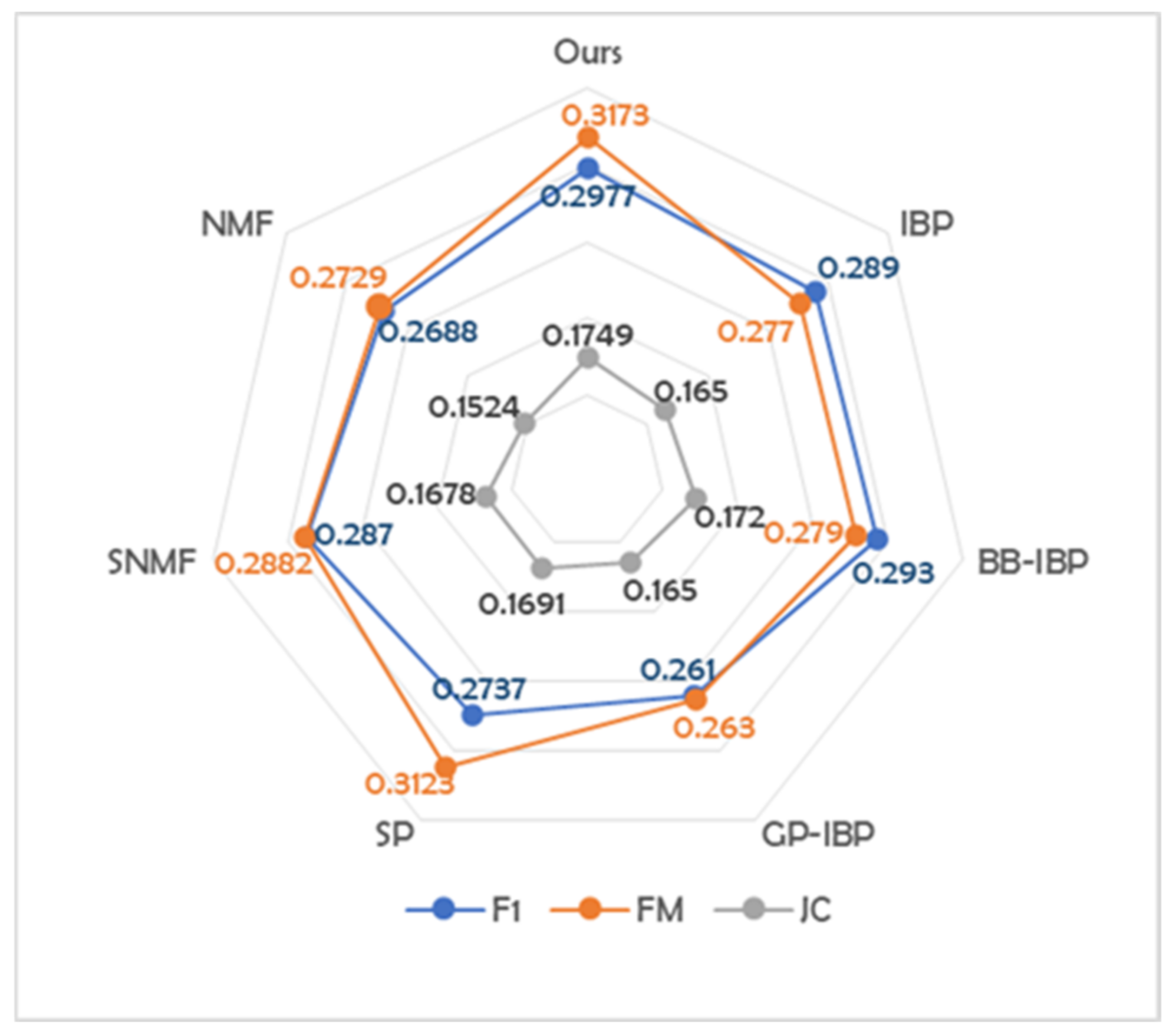
Figure 1. Non-negative matrix factorization with a single binary component.
Mathematics 09 01189 g001
Figure 2. The exponential Gaussian model.
Mathematics 09 01189 g002
Figure 3. Illustration of Indian Buffet process.
Mathematics 09 01189 g003
Figure 4. Approximate variational distribution diagram.
Mathematics 09 01189 g004
Figure 5. The analysis and reconstruction results on synthetic dataset: (a) the binary matrix Z , (b) the extracted latent features, (c) the original sample, (d) the reconstructed result. Here the white part indicates that the object has this feature while the black part indicates the opposite.
Mathematics 09 01189 g005
Figure 6. Samples of the swimmer dataset.
Mathematics 09 01189 g006
Figure 7. The extracted latent feature information.
Mathematics 09 01189 g007
Figure 8. Analysis and comparison results on swimmer dataset: (a) basic NMF decomposition results, (b) the comparative decomposition results including various combinations of limbs and the trunk.
Mathematics 09 01189 g008
Figure 9. Binary matrix Z of the swimmer dataset.
Mathematics 09 01189 g009
Figure 10. Comparative display of clustering results related to Cora dataset.
Mathematics 09 01189 g010
Figure 11. The samples of CBCL Face Database.
Mathematics 09 01189 g011
Figure 12. Extracted local features of human face.
Mathematics 09 01189 g012
Figure 13. Comparison of original face and reconstructed result.
Mathematics 09 01189 g013
Table 1. Clustering result of the Cora dataset.
IndexJCFMF1
Parametric Model or AlgorithmsSNMF0.1678 0.28820.2870
NMF0.1524 0.27290.2688
SP0.16910.31230.2737
Bayesian Non-parametric NMF ModelsIBP0.16500.27700.2890
Bivariate-Beta doubly IBP0.17200.27900.2930
Gaussian process doubly IBP0.16500.26300.2610
Ours0.17490.31730.2977
Publisher’s Note: MDPI stays neutral with regard to jurisdictional claims in published maps and institutional affiliations.

