Article

Using Markov Models to Characterize and Predict Process Target Compliance

School of Computing, Ulster University, Belfast BT37 0QB, Northern Ireland, UK
Mathematics 2021, 9(11), 1187; https://doi.org/10.3390/math9111187
Submission received: 7 May 2021 / Revised: 19 May 2021 / Accepted: 21 May 2021 / Published: 24 May 2021

Abstract

:
Processes are everywhere, covering disparate fields such as business, industry, telecommunications, and healthcare. They have previously been analyzed and modelled with the aim of improving understanding and efficiency as well as predicting future events and outcomes. In recent years, process mining has appeared with the aim of uncovering, observing, and improving processes, often based on data obtained from logs. This typically requires task identification, predicting future pathways, or identifying anomalies. We here concentrate on using Markov processes to assess compliance with completion targets or, inversely, we can determine appropriate targets for satisfactory performance. Previous work is extended to processes where there are a number of possible exit options, with potentially different target completion times. In particular, we look at distributions of the number of patients failing to meet targets, through time. The formulae are illustrated using data from a stroke patient unit, where there are multiple discharge destinations for patients, namely death, private nursing home, or the patient’s own home, where different discharge destinations may require disparate targets. Key performance indicators (KPIs) of this sort are commonplace in healthcare, business, and industrial processes. Markov models, or their extensions, have an important role to play in this work where the approach can be extended to include more expressive assumptions, with the aim of assessing compliance in complex scenarios.

1. Introduction

Processes are widespread, encompassing disparate areas such as business, production, telecommunications, and healthcare. They have previously been analyzed and modelled with the aim of improving understanding and efficiency as well as predicting future events and outcomes. With the burgeoning capability of IT systems to collect, process, store, and exchange data, and the upsurge of suitable technologies for Big Data, recently, process mining has appeared, providing a bridge between data mining and process modelling [1]. Process mining provides an opportunity and framework for service design and improvement, as well as a scientific rationale for decision-making. In general, we consider processes comprising several tasks each with start and end times and associated durations. A process instance completes these tasks according to the logic and rules prevailing in the real-world setting. The process data features mainly consist of data such as duration, customer id, etc., and are held in log files. Hence, such log files provide an automated time-stamped record of tasks performed during the execution of a given process.
Consequently, process mining may include discovering the tasks and trajectories that comprise the process, predicting trajectories, or identifying anomalies. Such activities can employ traditional methods for data mining such as classification, clustering, regression, association rules, sequence mining, or deep learning. However, model-based approaches can also provide opportunities for incorporating structural process knowledge into the analysis, thereby facilitating improved understanding and prediction. As such, process mining can be employed in diverse areas, such as manufacturing [2], telecommunications [3], financial processing, and healthcare [4].
A mathematical model is often used as a simplified version of a process, where simulation uses the model to imitate the behaviour of the process, without interfering with the actual process [5]. Correctness, conformance, and performance are some of the most important problems for complex processes, where models have often been used to resolve such issues. Performance analysis typically focuses on the dynamic behaviour of the process, based on metrics such as response time, uptime, or output. Our emphasis here is on measuring if a process meets its targets. For example, a business process might have order completion targets to meet, and an accident and emergency department could have discharge targets, while service-level agreements (SLAs) are commonly used to characterize cloud performance targets.
(Stochastic) process algebras have been implemented in formal languages to describe a system model. For example, Petri nets [6] were introduced by Carl Adam Petri in 1962 to characterize and analyze concurrent systems. They are based on mathematical specification alongside a mathematical theory for interpretation and analysis. For example, Petri nets have been used for workflow modelling [7]. In addition, stochastic Petri nets [8], including queueing Petri nets, have been developed.
A Markov model is a type of probabilistic process model that can describe such systems where it is assumed that the Markov property is followed, i.e., future states only depend on present states, and not additionally on previous ones. This enables both individual probabilistic predictive modelling [9] and group forecasting for individuals moving through a process [10]. Higher-order Markov models may alternatively be employed if the Markov assumption is not appropriate. In addition, continuous-time Markov chains (CTMCs) are commonly used where the Markov property translates into exponentially distributed durations. Such models can be used to find “interesting” (in)frequent pathways [11].
In this paper, we extend our previous initial work on using Markov models to predict process target compliance [12]. Several formulae are obtained and used for a process concerning stroke patient pathways achieving targets for the duration of hospitalization and subsequent discharge to different types of community care. In what follows, we formulate the problem for a general phase-type Markov model, where previously we focus on Coxian models. We also extend the work to situations where there are multiple absorbing (discharge) states and also for groups of individuals (e.g., patients) moving through the system towards discharge targets.

2. Background

Markov models have been used to represent various types of process applications, including call centres [13], sensor networks [14], telecommunications [15], production modelling [16] and healthcare [10]. Phase-type models are a special case of a Markov model where there are transient states (or phases) and, typically, a single absorbing state where generally the interest is in duration of stay in the set of transient states. In healthcare, we typically have some hospital states followed by one, or more, absorbing states in the community. These models can be used to predict individual patient movements or to predict future resource requirements or costs for groups of patients [17]. They facilitate conceptualization of flows, e.g., for hospital patients, through testing, diagnosis, treatment, and rehabilitation. Such phase-type distributions (PHDs) can be utilized to describe duration in a group of states where the PHD represents the time from admission to the transient states until absorption into the absorbing state. In particular, Coxian phase-type distributions (C-PHDs) are a useful special case where a process always starts in the first transient state and can never return to a state once it has left it. Transition from a transient state to the absorbing state is also allowed (Figure 1). Such PHDs provide a simple model for a key performance indicator (KPI) such as length of stay in the transient states, e.g., duration of a particular activity, or from order placement to delivery. Parameter estimation for PHDs is also typically straightforward [9]. In general, phase-type models (PHDs) are well suited to a range of situations, including healthcare [18,19,20,21], community care [22], accident and emergency [23], and activity recognition [24]. They are also understandable as we can conceptualize a patient or customer as moving through the phases.
In addition, PHDs have the following advantages: (i) their mathematical simplicity; (ii) parsimonious parameterization; (iii) flexibility in terms of fitting different shapes of distribution; and (iv) ease of migration to more complex settings, either using a mathematical or simulation approach.
In the current paper, as in our previous work, e.g., [25,26], we include covariates, or additional features, into the model by allowing the initial and transition probabilities to depend explicitly on these covariates. The specific functional form of these covariate models will be described in the next section.

3. Phase-Type Models

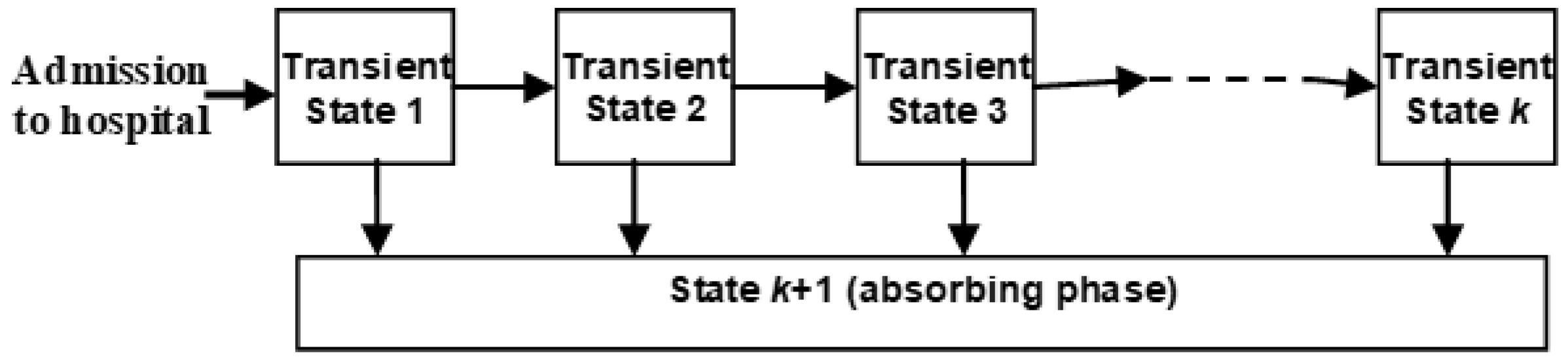
3.1. The Basic Phase-Type Model

As in [5,12], we use here a phase-type Markov process model. This representation of a process by a Markov, or more specifically, a phase-type model allows us to incorporate variability into process tasks, thus facilitating implementation and adaptation. As discussed, the phase-type model provides a useful way of describing process duration and also has other advantages, such as computational efficiency.
We begin by defining k transient phases S1, …, Sk, with phase Sk+1 being the only absorbing state. Writing the initial vector as: α = ( α 1 , α k ) , where αi is the probability of entry to phase Si for i = 1, …, k, we obtain the probability density function (p.d.f.) of the distribution of duration until transition to the absorbing state as:
f ( x ) = α   exp   ( T x ) t A ,
where T = {tij} is the k × k generator matrix for the transition rates between the transient states and i = 1, …, k, j = 1, …, k. Here, t A is the column vector of transition rates from the transient states to the absorbing state and t A = T 1 where 1 is a column vector of 1’s, pointing to the fact that the row sums of the generator matrix are zero.
Integrating the p.d.f., we obtain the cumulative distribution function (c.d.f.) as
F X ( y ;   α ,   T )   = 1 α   exp   ( T y ) 1 ; y 0 .
which describes the probability of meeting a given duration target y for length of stay in the transient states. Similarly, the probability of missing a duration target y is given by
F ¯ x ( y ;   α ,   T )   = α   exp   ( T y ) 1 ; y 0 .
We note that the inverse problem of ascertaining an appropriate duration target, given a required percentage compliance, can be obtained from Equation (3) by solving to find y for a given F. Here F can be a service-level agreement in a management or industrial context. So, for example, we may require that 95% of tasks are completed within a given target duration in the transient states. Although we cannot solve Equation (3) explicitly for y, we can a use a numerical solution, such as Newton–Raphson, where the estimate of y is given at the (n + 1)th iteration by
y n + 1 = y n F ( y n ) / F ( y n ) ,
where F ( y n ) = α   exp ( T y n ) T 1 .
In this way, we can not only characterize the relative likelihoods of compliance and non-compliance with a target but also consider the most likely state trajectories. Using the approach of [26], we determine the conditional probability of meeting (or otherwise) a target of duration y given that an amount of time d has already passed. This probability is given by
F X | X > d ( y ;   α ,   T )   =   1 α   exp   ( T y ) 1 α   exp   ( T d ) 1 ; y d ,
which represents the probability of meeting a given target y. Also, the probability of missing a target y is given by
F ¯ X | X > d ( y ;   α ,   T )   =   α   exp   ( T y ) 1 α   exp   ( T d ) 1 ; y d .
In a similar manner, conditional means can be calculated by integrating the conditional densities, as previously discussed in McClean et al. [12].

3.2. Multiple Absorbing States with Different Targets

To date, we have assumed that the target for absorption will be the same, irrespective of the initial state. While this may be the case in many situations, it is clearly not always the case. For example, for stroke patients, as we will discuss in our case study, the three initial states are (1) haemorrhagic stroke, (2) cerebral infarction stroke, and (3) transitory ischaemic attack (TIA). However, in this example, the anticipated length of stay in hospital depends on the type of stroke, with haemorrhagic stroke being more severe than cerebral infarction and cerebral infarction being more severe than TIA. In addition, the expected length of stay will vary with the discharge destination, with more severe strokes leading to destinations which require community settings which provide more support for the patient. This observation underpins our model, where we assume that the patients progress from one transient state (phase) to another less severe one. It is therefore likely that, for such situations, the individual targets will differ across initial phases. So, for the stroke patient example, we might expect the target for haemorrhagic patients to be greater than that of cerebral infarction patients and the target for cerebral infarction patients should be larger than that for TIA patients, corresponding to greater stroke severity generally requiring longer hospitalization.
Previously, we extended this model to incorporate the occurrence of multiple absorbing states into the phase-type model [26], as follows.
The infinitesimal generator matrix Q is given by
Q ( x ) = ( T ( x ) t A ( x ) 0 A T 0 A A ) .
Here T = {tij} is a k × k matrix of transition rates between the k transient states, given by
T ( x ) = ( Λ 1 ( x ) λ 1 k ( x ) 0 Λ k ( x ) ) ,
where Λ i ( x ) = j = 2 k λ i j ( x ) + j = 1 m μ i j ( x ) .
Here we allow the transition rates to depend on covariates x = {xi}; for example, for stroke patients these could be age and gender, where the μ i j ( x ) terms represent transition rates from transient state Si to absorbing state Sj for i = 1, …, k and j = 1, …, m, and m represents the number of absorbing states. The k × m matrix tA is then given by tA = { μ i j ( x ) }.
Finally, 0AT and 0AA are zero matrices of suitable dimensions and 0 is a zero column vector. These elements satisfy the conditions tii < 0 for I = 1, …, k and tij ≥ 0 for i = 1, …, k; for j = 1, …m. Also, T and tA satisfy tA1m = −T1k where 1m is an m-dimensional column vector of ones.
In a similar way to Equation (1) we obtain f(t) = {fi(t)} where fi(t) is the unconditional (degenerate) p.d.f. of the time spent in the transient states prior to discharge to absorbing state Sk+i for i = 1, …, m, and
f ( t ) = α   exp   ( T t ) t A
The probability of meeting target τ i for absorbing state Sk+i is therefore given by
M i ( τ i ;   α ,   T )   = 0 τ i α   exp ( T y ) t A   I i d y ; y 0 ,   i = 1 ,   ,   m ,
where I i is an m-dimensional column vector with 1 in the ith position and zeros elsewhere; t A   I i is therefore the ith column of t A .
Integrating this expression, we obtain
M i ( τ i ;   α ,   T )   = { α   exp ( T τ i ) T 1 t A   I i α   T 1 t A   I i } = α   ( I exp ( T τ i ) ) ( T 1 ) t A   I i     i = 1 ,   ,   m .
Here, when the targets are equal across all absorbing states, i.e., τ i = τ     i , the total probability of meeting the target is i = 1 m M i ( τ ;   α ,   T ) = α   exp   ( T τ ) 1 , as for Equation (3).
We note that these formulae, for the probability of meeting targets when there are multiple “risks”, are related to those used in epidemiology for cumulative incidence, e.g., [27].
We can also obtain the conditional probability of meeting the target τ i for the absorbing state Sk+i, given eventual absorption is to this state, which is given by
L i ( τ i ;   α ,   T ) = { α   ( I exp ( T τ i ) ) ( T 1 ) t A   I i } / { α   ( T 1 ) t A   I i }     i = 1 ,   ,   m .
This expression is useful in terms of allowing us to determine the profile of different groups of patients characterized by their final destination and quantifying how likely they are to meet the given possible targets with regard to duration in the transient states. While our previous expressions are more geared towards making and meeting targets for individuals, Equation (12) allows us to move towards thinking about cohorts of individuals meeting overall targets for the system of transient states. For example, in the stroke patient situation we explore below, the performance of a stroke unit in terms of meeting hospital targets can be measured in terms of the different discharge destinations (absorbing states), namely death, private nursing home and own homes. Mathematically, this is achieved through the entry vector α , which here represents an overall probability distribution across the different types of stroke. We now focus further on such population models for setting targets.

3.3. Poisson Arrivals

So far, we have considered individual movements through the transient states, with eventual absorption into one of a number of possible exit states. Our focus here has thus been on providing expressions for target achievement. However, for such processes, there is often an interest in characterizing the movements of a number of individuals moving through the system in parallel where, for example, we may want to characterize and/or predict the numbers of individuals attaining a target in a given time interval. As such, our focus now shifts to a Markov system; for further details of such systems and a discussion of various possible extensions, see, for example, [28].
We consider a situation where new arrivals to the Markov process occur according to a Poisson process, rate ω where we have an initial probability vector α, k transient states, and one absorbing state, as before. We are interested in determining the probability distribution of the number of individuals arriving in time interval (0, ∞) who fail to meet a fixed target d.
Let M(t) be the number of individuals who arrive in (0, t) according to a Poisson process, rate ω, and fail to comply. Each of these individuals fails to comply with probability Φ where Φ = α exp { T d }   1 k , using Equation (3). Then, the distribution of N(t), the total number of arrivals in (0, d), is Poisson (ωd) and the distribution of M(d) is a compound distribution, consisting of a binomial choice from a Poisson number of failures.
The probability generating function (p.g.f.) of a r.v. N~Poisson(ωt) is given by EN[zN] = G(z) = exp(ωd (z − 1)), and the p.g.f. of a random variable (r.v.) M~Binomial (N, p) is EM[zM] = G(z) = (q + pz)M, where q = 1 − p. The p.g.f. of the required compound distribution is therefore
H M ( z ) = E N [ E M [ z M | N ] ] = G ( F ( z ) ) = exp {   ω d   ( ( 1 Φ ) + Φ z ) 1 ) } = exp {   ω d   Φ ( z 1 ) } .
So, the number of failures who comply with target d from individuals arriving in (0, t) is a Poisson with mean (and variance):
ω t   α exp { T d }   1 k .
Similarly to the situation considered previously, where we have m absorbing states, we again have a compound distribution of a Poisson (arrival) rate ω and a binomial (transition to absorbing state i after duration di). Then, integrating Equation (12) we obtain the result that the number of individuals arriving in (0, t) who meet target di for absorbing state Sk+i is a Poisson with mean (and variance):
ω t { α   ( I exp ( T τ i ) ) ( T 1 ) t A   I i } ,
where I i is an m-dimensional column vector with 1 in the ith position, as before.
Based on this result, we can understand and predict the variability of numbers of individuals moving through the transient states in terms of their likelihood of meeting targets. The mathematical development in this section suggests that such variability is likely to be high and increase with time. This further highlights the importance of setting achievable targets.

4. Results

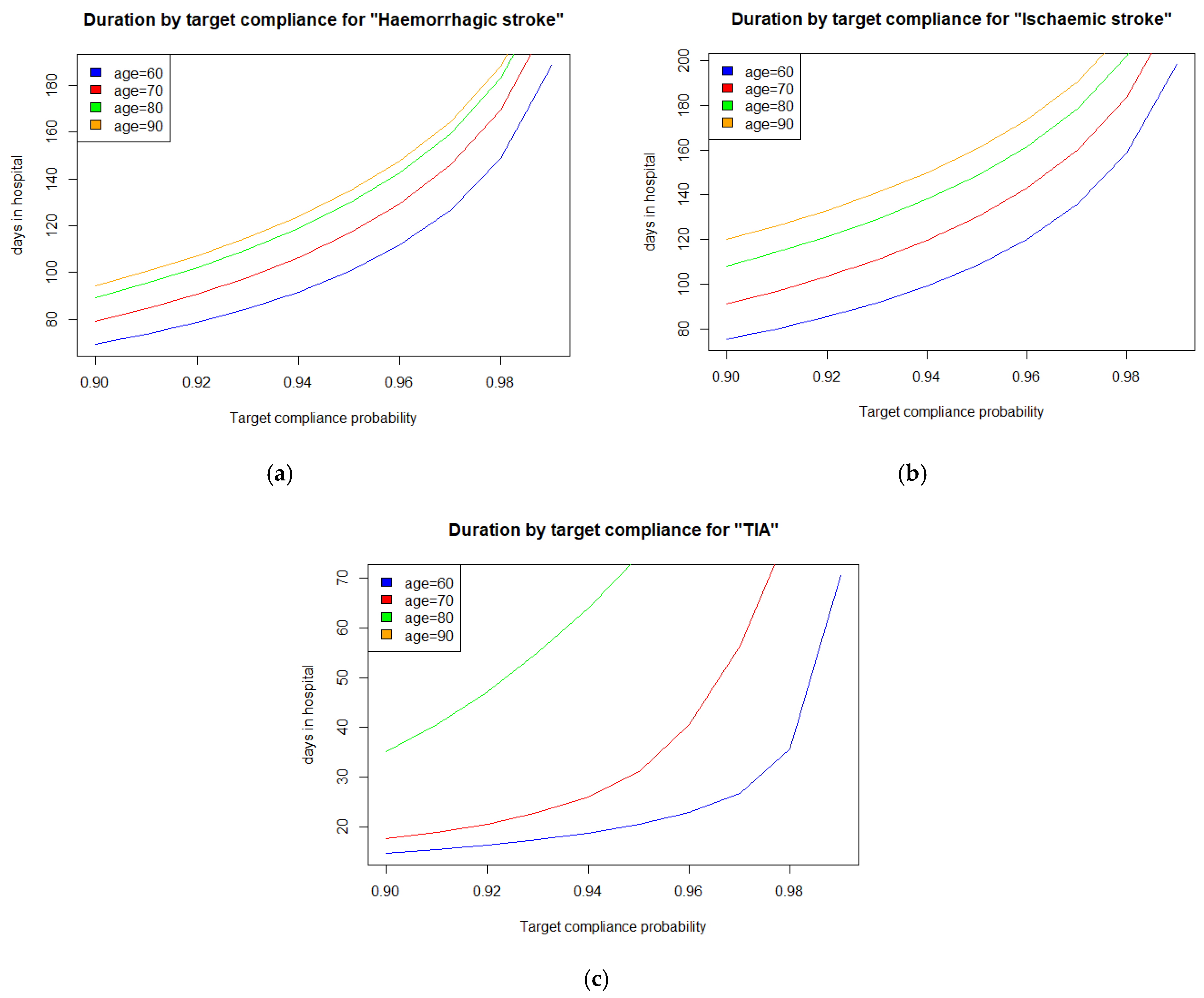
4.1. The Stroke Care Case Study

In practice, it is often the case that a number of absorbing states are possible, with possibly different targets. Previously, we have discussed phase-type models which contain multiple absorbing states [5,26]. We now apply our model to such a situation involving stroke patients using data spreading over 5 years. Here, we have described a phase-type model with four transient states corresponding to different types of stroke with contrasting severity and related admission probabilities for differing stroke severity. The data contain three types of stroke: haemorrhagic (the most severe, caused by bleeding in the brain), cerebral infarction (less severe, due to blood clots), and transient ischaemic attack or TIA (the least severe, a minor stroke caused by a small clot). Following hospitalization, there are three possible discharge destinations: (1) following the patient’s death, (2) with a discharge to a private nursing home, and (3) with a discharge to the patient’s own home. These different situations can be described by defining the exit matrix tA as
t A   = ( μ 1 ν 1 ρ 1 μ 2 ν 2 ρ 2 μ 3 ν 3 ρ 3 μ 4 ν 4 ρ 4 )
For this special case of t A , each column relates to a different hospital discharge event, while the rows correspond to the transient phases of hospitalization [26].
In this study, data were collected over a 5-year period, on admission date, discharge date, diagnosis on admission, and discharge destination, alongside other covariates, such as age on admission and gender. The transition rates of the model may depend upon the age and stroke type of the patient, or may not depend on age [5]. We note in passing that the Poisson admission assumption was previously tested using chi-square and Kolmogorov–Smirnov tests and shown to be acceptable for our Belfast City Hospital stroke patient data [5].
So far, we have not discussed the possibility of covariates playing a significant role in the Markov model. However, as is often the case, for the stroke patient case we have additional covariates, namely age and gender. In our previous work, we determined that while gender does not have a significant effect, age does and has therefore been included in the model, as follows. Other covariates were not available for this dataset but, in general, the results of tests or diagnostics might be relevant covariates.
For i = 1, 2, let λi(x) be the transition intensity from phase Si to phase Si+1 for a patient of age x, where λ i ( x ) = e x p ( γ i + β i   x ) . Also, p(x) is the probability that a TIA patient aged x enters phase S4 upon admission to hospital, representing the least severe type of stroke. Consequently, a more severe TIA patient starts in phase S3 with probability 1 − p(x). We assume that p(x) = exp{−exp(θ0 + θ1 x)}. The exponential functions here used in modelling λi(x) and (x) are standard representations, which constrain the probability values to the required ranges. Such functions are found in the literature for log link and complementary log–log link functions for generalized linear models, e.g., [29]. As seen in Figure 2, it is assumed that µ4 = ν4 = 0, representing the fact that patients with a minor TIA (S4) are always discharged to their own home. Similarly, for the other transitions from the transient phases (S1, S2, and S3) to each absorbing state, we assume that ν1 = p1 = 0. We note that transitions absent in Figure 2, and corresponding zero parameters, have been found by statistical testing based on likelihood ratio tests; for further details, see [26].

4.2. Findings

The following findings are based on model parameter values as described in [26]. These were estimated using a 5-year retrospective dataset consisting of 1985 patients. Figure 3 presents the cumulative probability of discharge from hospital by age for (a) haemorrhagic stroke, (b) cerebral infarction, and (c) TIA. The 95% compliance is also presented in these plots to make it easier to evaluate the compliance target, in days, for a commonly used compliance probability. In all three plots, we can see that the older the patient, the longer the stay in hospital and the less likely patients are to comply with a given target, as expected. Here, we see that, for a given compliance probability, the haemorrhagic patients typically spend much longer in hospital and, similarly, TIA patients spend much shorter periods in hospitals, so a lower target would be appropriate for them. This is as we would anticipate, with more serious, or more infirm, patients staying longer in hospital. Patients with cerebral infarction are intermediate, in this regard, as we would expect.
In Figure 4 we present the duration of stay in hospital by age for compliance with different targets for (a) haemorrhagic stroke, (b) cerebral infarction, and (c) TIA. We see from the plots that, as before, the more serious the stroke, the longer the patients need to be allocated to reach a given target, as prolonged rehabilitation is needed for such patients to move through the different treatment and recovery phases before discharge. Moreover, as the targets become more severe, they become increasingly harder to achieve, for all patients.
In Figure 4 we present the duration of stay in hospital by age for compliance with different targets for (a) haemorrhagic stroke, (b) cerebral infarction, and (c) TIA. We see from the plots that, as before, the more serious the stroke, the longer the patients need to be given to reach a given target, as a longer period of rehabilitation is required for these patients to move through the treatment and recovery phases prior to discharge. Also, as the targets become more severe, they become increasingly harder to achieve, for all patients.
Figure 5 presents cumulative conditional probability of discharge from hospital by age conditional on eventual discharge to (a) death, (b) private nursing home, and (c) own home. We note that the admission vector here is across the population of stroke patients from all types of stroke, as we are thinking in terms of setting targets for the stroke unit rather than individual patients, as before. As we can see, these profiles are quite different across discharge distributions, highlighting the importance of different targets for private nursing homes and own homes. We have presented the graph for deaths in hospital as well for interest, although a target would be inappropriate here. Looking at the plots, we see that the longest durations are for patients who are discharged to their own home. The shortest are those who die in hospital, while those discharged to private nursing home are intermediate. This is reasonable as the patients who die in hospital are mainly very ill when they are admitted, while patients who are discharged to private nursing home are also quite ill and need a lot of rehabilitation before discharge. The patients who die do not display much variation between age groups, while older patients discharged to their home require longer periods in hospital than younger such patients, as they probably require more rehabilitation than younger patients. It is interesting that this age effect is reversed in patients discharged to private nursing homes, possibly because more time is spent trying unsuccessfully to rehabilitate them to a stage when they might manage at home, with a package.

5. Discussion

In our stroke patient example, Markov models can be used to describe the stroke patient care system using well-known clinical pathways, which integrate hospital and community services to provide ways of characterizing services, evaluating planned transformations, and predicting resourcing needs for future situations. Our previous paper [26] developed approaches to utilize routinely available discharge data to characterize patient admission patterns, movements through care, and release to suitable destinations. Such an approach can assist performance modelling, bed occupancy analysis, capacity planning, and patient destination prediction across different sectors of the patient care system. By using such an approach, we can compare different options and identify optimal policies. We note that stroke patient care provides an important paradigm example for healthcare processes generally, as there are numerous other specialties that encompass hospital and community services. Overall consumption of hospital resources and compliance with related targets are KPIs for healthcare services, and tools are thus needed to assess the effect of policies and their impact on patient hospitalization targets.

6. Conclusions

This paper described how process mining can provide suitable data from suitable datasets to populate phase-type models, which can then be used to quantify compliance with process targets or identify suitable targets given a required compliance percentage We described an example that uses phase-type models to describe stroke patient hospitalization and discharge, where there are multiple discharge destinations. Based on this use-case, various options have been investigated, with an emphasis on measuring target compliance; such performance indicators are frequently used in healthcare settings as well as in business and industrial environments. Multiple absorbing states quite commonly occur in such application domains. For example, there is an extensive literature on using Markov models for breast cancer patients where multiple absorbing states may come from different outcomes or using stratification to represent different characteristics of the patients [30].
Our current approach is part of initial efforts towards developing integrated process models, with the aim of supporting integrated management, planning, and resourcing. An important aspect of extending our framework, as described, is that it allows us to find the probability distribution of target compliance for multiple absorbing states and use Poisson processes to model arrivals; costs can also be associated with various parts of the system.
The approach is likely to be pertinent to business processes generally where phase-type models should have an important role to play.

Funding

This research was partly funded by the Invest Northern Ireland BTIIC project (BT Ireland Innovation Centre).

Institutional Review Board Statement

Not applicable.

Informed Consent Statement

Not applicable.

Data Availability Statement

Not applicable.

Conflicts of Interest

The author declares no conflict of interest. The funders had no role in the design of the study; in the collection, analyses, or interpretation of data; in the writing of the manuscript; or in the decision to publish the results.

References

  1. Van der Aalst, W. Process mining: Overview and opportunities. ACM TMIS 2012, 3, 7. [Google Scholar] [CrossRef]
  2. Van der Aalst, W.; Reijers, H.; Weijters, A.; van Dongen, B.; de Medeiros, A.A.; Song, M.; Verbeek, H. Business process mining: An industrial application. Inf. Syst. 2007, 32, 713–732. [Google Scholar] [CrossRef]
  3. Taylor, P. Autonomic Business Processes. Ph.D. Thesis, University of York, York, UK, 2015. [Google Scholar]
  4. Agrawal, R.; Imieliński, T.; Swami, A. Mining association rules between sets of items in large databases. ACM SIGMOD Rec. 1993, 22, 207–216. [Google Scholar] [CrossRef]
  5. McClean, S.; Barton, M.; Garg, L.; Fullerton, K. A modeling framework that combines markov models and discrete-event simulation for stroke patient care. ACM Trans. Model. Comput. Simul. 2011, 21, 1–26. [Google Scholar] [CrossRef]
  6. Peterson, J.L. Petri Net Theory and the Modeling of Systems; Prentice Hall PTR: Hoboken, FL, USA, 1981. [Google Scholar]
  7. McChesney, I. Process support for continuous, distributed, multi-party healthcare processes—applying workflow modelling to an anticoagulation monitoring protocol. In Proceedings of the 10th International Conference on Ubiquitous Computing and Ambient Intelligence, Las Palmas de Gran Canaria, Spain, 29 November—2 December 2016; Springer: Berlin/Heidelberg, Germany, 2016; p. 255. [Google Scholar]
  8. Haas, P.J. Stochastic Petri Nets: Modelling, Stability, Simulation; Springer Science & Business Media: Berlin/Heidelbaerg, Germany, 2016; p. 10. [Google Scholar]
  9. Garg, L.; McClean, S.I.; Barton, M.; Meenan, B.J.; Fullerton, K. Intelligent Patient Management and Resource Planning for Complex, Heterogeneous, and Stochastic Healthcare Systems. IEEE Trans. Syst. Man Cybern. Part A Syst. Humans 2012, 42, 1332–1345. [Google Scholar] [CrossRef]
  10. Gillespie, J.; McClean, S.; Garg, L.; Barton, M.; Scotney, B.; Fullerton, K. A multi-phase des modelling framework for pa-tient-centred care. JORS 2016, 67, 1239–1249. [Google Scholar]
  11. Garg, L.; McClean, S.; Meenan, B.; Millard, P. Non-homogeneous Markov models for sequential pattern mining of healthcare data. IMA J. Manag. Math. 2008, 20, 327–344. [Google Scholar] [CrossRef]
  12. McClean, S.; Stanford, D.; Garg, L.; Khan, N. Using Phase-type Models to Monitor and Predict Process Target Compliance. Proc. Int. Conf. Oper. Res. Enterpr. Syst. 2019, 2019, 82–90. [Google Scholar] [CrossRef]
  13. Dudin, A.; Kim, C.; Dudina, O.; Dudin, S. Multi-server queueing system with a generalized phase-type service time dis-tribution as a model of call center with a call-back option. Ann. Oper. Res. 2016, 239, 401–428. [Google Scholar] [CrossRef]
  14. Dudin, S.A.; Lee, M.H. Analysis of Single-Server Queue with Phase-Type Service and Energy Harvesting. Math. Probl. Eng. 2016, 2016, 1–16. [Google Scholar] [CrossRef] [Green Version]
  15. Vishnevskii, V.M.; Dudin, A.N. Queueing systems with correlated arrival flows and their applications to modeling tele-communication networks. Autom. Remote Control 2017, 78, 1361–1403. [Google Scholar] [CrossRef]
  16. Barron, Y.; Perry, D.; Stadje, W. A make-tostock production/inventory model with map arrivals and phase-type demands. Ann. Oper. Res. 2016, 241, 373–409. [Google Scholar] [CrossRef]
  17. McClean, S.; Gillespie, J.; Garg, L.; Barton, M.; Scotney, B.; Kullerton, K. Using phase-type models to cost stroke patient care across health, social and community services. Eur. J. Oper. Res. 2014, 236, 190–199. [Google Scholar] [CrossRef]
  18. Fackrell, M. Modelling healthcare systems with phase-type distributions. Heal. Care Manag. Sci. 2008, 12, 11–26. [Google Scholar] [CrossRef] [PubMed]
  19. Tang, X.; Luo, Z.; Gardiner, J.C. Modeling hospital length of stay by Coxian phase-type regression with heterogeneity. Stat. Med. 2012, 31, 1502–1516. [Google Scholar] [CrossRef]
  20. Marshall, A.H.; Zenga, M. Experimenting with the Coxian Phase-Type Distribution to Uncover Suitable Fits. Methodol. Comput. Appl. Probab. 2010, 14, 71–86. [Google Scholar] [CrossRef]
  21. Griffiths, J.; Williams, J.; Wood, R. Modelling activities at a neurological rehabilitation unit. Eur. J. Oper. Res. 2013, 226, 301–312. [Google Scholar] [CrossRef]
  22. Xie, H.; Chaussalet, T.; Millard, P. A Model-Based Approach to the Analysis of Patterns of Length of Stay in Institutional Long-Term Care. IEEE Trans. Inf. Technol. Biomed. 2006, 10, 512–518. [Google Scholar] [CrossRef] [Green Version]
  23. Knight, V.A.; Harper, P.R. Modelling emergency medical services with phase-type distributions. Heal. Syst. 2012, 1, 58–68. [Google Scholar] [CrossRef]
  24. Duong, T.; Phung, D.; Bui, H.H.; Venkatesh, S. Efficient duration and hierarchical modeling for human activity recogni-tion. Artif. Intell. 2009, 173, 830–856. [Google Scholar] [CrossRef] [Green Version]
  25. Faddy, M.J.; McClean, S.I. Markov Chain Modelling for Geriatric Patient Care. Methods Inf. Med. 2005, 44, 369–373. [Google Scholar] [CrossRef] [PubMed]
  26. Jones, B.; McClean, S.; Stanford, D. Modelling mortality and discharge of hospitalized stroke patients using a phase-type recovery model. HCMS 2018, 22, 1–19. [Google Scholar] [CrossRef] [PubMed] [Green Version]
  27. McClean, S.; Gribbin, O. A non-parametric competing risks model for manpower planning. Appl. Stoch. Model. Data Anal. 1991, 7, 327–341. [Google Scholar] [CrossRef]
  28. Vassiliou, P.-C.G. Rate of Convergence and Periodicity of the Expected Population Structure of Markov Systems that Live in a General State Space. Mathematics 2020, 8, 1021. [Google Scholar] [CrossRef]
  29. Dobson, A.J.; Barnett, A.G. An Introduction to Generalized Linear Models; CRC Press: Boca Raton, FL, USA, 2008. [Google Scholar]
  30. Otten, M.; Timmer, J.; Witteveen, A. Stratified breast cancer follow-up using a continuous state partially observable Markov decision process. Eur. J. Oper. Res. 2020, 281, 464–474. [Google Scholar] [CrossRef] [Green Version]
Figure 1. A k state patient Coxian phase-type distribution.
Mathematics 09 01187 g001
Figure 2. Stroke care transition diagram.
Mathematics 09 01187 g002
Figure 3. Cumulative probability of discharge from hospital by age for (a) haemorrhagic stroke, (b) cerebral infarction, and (c) TIA.
Mathematics 09 01187 g003
Figure 4. Duration of stay in hospital by age for compliance with different targets for (a) haemorrhagic stroke, (b) cerebral infarction, and (c) TIA.
Mathematics 09 01187 g004
Figure 5. Cumulative conditional probability of discharge from hospital by age conditional on eventual discharge to (a) death, (b) private nursing home, and (c) own home.
Mathematics 09 01187 g005
Publisher’s Note: MDPI stays neutral with regard to jurisdictional claims in published maps and institutional affiliations.

