Thermal Conductivity Estimation Based on Well Logging

Abstract

The thermal conductivity of a stratum is a key factor to study the deep temperature distribution and the thermal structure of the basin. A huge expense of core sampling from boreholes, especially in offshore areas, makes it expensive to directly test stratum samples. Therefore, the use of well logging (the gamma-ray, the neutron porosity, and the temperature) to estimate the thermal conductivity of the samples obtained from boreholes could be a good alternative. In this study, we measured the thermal conductivity of 72 samples obtained from an offshore area as references. When the stratum is considered to be a shale–sand–fluid model, the thermal conductivity can be calculated based on the mixing models (the geometric mean and the square root mean). The contents of the shale and the sand were derived from the natural gamma-ray logs, and the content of the fluid (porosity) was derived from the neutron porosity logs. The temperature corrections of the thermal conductivity were performed for the solid component and the fluid component separately. By comparing with the measured data, the thermal conductivity predicted based on the square root model showed good consistency. This technique is low-cost and has great potential to be used as an application method to obtain the thermal conductivity for geothermal research.

1. Introduction

The thermal conductivity (TC) of rocks is a measure of their ability to conduct heat. It is defined as the quantity of heat that passes in the unit time through a plate with a certain area and thickness whose opposite faces have a temperature difference of one kelvin [1]. There are two ways to obtain the TC of rocks: (1) the direct way to test a rock sample in a laboratory to measure it, and (2) the indirect way to calculate it based on geophysical well logging employing appropriate models.

Laboratory measures are relatively more accurate and reliable; however, there are also some deficiencies. Firstly, borehole samples are rare and not easy to obtain. Additionally, limited and discontinued samples cannot provide enough information or represent the study area. Further, there could be some small fractures in the rock samples because of the released stress, which will cause analytical errors of the testing. Using the well logging data to determine the TC of the borehole rocks is fast and economical, and more importantly, it can reflect the in situ properties. For determining TC, an empirical relationship was derived based on the sonic velocity or the bulk density in California [2]. However, it sometimes does not work well in other study areas and lacks physical principles. Our goal of this paper is to develop a quantitative prediction model of TC based on well logging, including gamma-ray, neutron porosity, and temperature logging.

Renewable energy is collected from a renewable resource, which is naturally replenished on a human timescale, including carbon neutral sources such as solar, wind, rain, tides, waves, and geothermal energy [3]. Geothermal energy is a clean and renewable energy source that can be found in abundance on earth [4].

In this study, we introduced a shale–sand–fluid model and used well logging, natural gamma ray and neutron porosity, to estimate the component proportions. Two mixing laws (geometry mean and square root mean) were considered in calculating the TC. Additionally, the temperature corrections of solid and water were performed separately based on the temperature logging data. The predicted TC has good agreement with the tested TC. TC is a key parameter in geothermal energy studies. Terrestrial heat flow at a given locality is the rate of heat transferred across Earth’s surface at that place per unit area per unit time [5]. Combining TC with temperature gradient, the heat flow can be determined [6]. Given enough heat flow data, we can obtain a contour map which can help us find the geothermal reservoir. Further, TC can be used to calculate the temperature field, which is the foundation of evaluating geothermal resources [7].

2. Thermal Conductivity Estimation

The TC of rocks can be influenced by other factors such as pressure, temperature, porosity, and fluid saturation [8]. According to the laboratory experiments, 2000 m buried depth can cause only a less than 2% increase in TC, which is within the analytical error of the laboratory testing [9,10], so the pressure has no significant influence on TC in the study area. Therefore, pressure correction was not considered in this paper.

2.1. Mixing Law

The mixing law was used to quantify the mean or effective TC value of in situ rock or formation [1]. The mixing model that can describe the geometry of rock or formation most accurately should be chosen to estimate the mean TC value. There are three important models to be considered: the harmonic mean, the arithmetic mean, and the geometric or square root mean.

The harmonic mean (Equation (1)) can be applied to bed layers whose heat flow is perpendicular to the layers. For example, this can apply to the vertical well drilled through the horizontal stratum. This is a weighted mean of the thermal resistance of each layer based on their proportions:

$$\frac{1}{k_B}={\displaystyle \sum }_i^n\frac{{\varphi }_i}{k_i}$$

(1)

where $k_B$ is the mean TC, and $k_i$ and ${\varphi }_i$ are TC and the proportion of the ith component, respectively.

If the heat flow transfers parallel to the layers like the faulting and the igneous intrusion, the arithmetic mean (Equation (2)) would be the best. This is a weighted mean TC of each layer based on their proportions:

$$k_B={\displaystyle \sum }_i^n{\varphi }_i{k}_i$$

(2)

The mean TC of a rock composed of different minerals is the most difficult to be described mathematically. Several components are randomly orientated and distributed in the rock. In this case, the geometric mean and the square root mean are most widely used to approximate the TC of a rock.

Beardsmore (2001) [1] suggested the geometric mean, which is the product of the TC of each component powered by its proportion:

$$k_B={\displaystyle \prod }_{i=i}^n{k}_i^{{\varphi }_i}$$

(3)

Roy et al. (1981) [11] suggested the use of the square root mean with a greater physical basis rather than the use of the geometric mean:

$$\sqrt{k_B}={\displaystyle \sum }_i^n{\varphi }_i\sqrt{k_i}$$

(4)

The difference between these two models is about 6–7%. Therefore, it is important to choose the most appropriate model. The square root mean based on physical principles is recommended unless there are some reasons to choose the other model.

2.2. Temperature Correction

The TC of rocks is sensitive to the temperature and the value of TC decreases with the increase in the temperature as governed by:

$$k\left(T\right)=\frac{T_0{T}_m}{T_m-T_0}\left(k_0-k_m\right)\left(\frac{1}{T}-\frac{1}{T_m}\right)+k_m$$

(5)

where $k_m$ is the calibration TC at $T_m\left(1.05 \mathrm{W}·{\mathrm{m}}^{-1}·{\mathrm{K}}^{-1}\right)$, $k_0$ is TC at the laboratory temperature $T_0$, $T_0$ is the laboratory temperature at which $k_0$ was measured (293 K in this study), and $T_m$ is the temperature at which $k_m$ was measured (1473 K) [12].

However, this equation is based on dry rocks. The TC of water is different from the TC of rocks and varies significantly with the temperature change as:

$$k_{water}=0.5706+1.756\times {10}^{-3}T-6.46\times {10}^{-6}{T}^2$$

(6)

where T is the temperature in °C within 0.3% error from the real TC value in the temperature range from °C to 200 °C [13].

3. Method

3.1. TC Measurements in a Laboratory

There are many ways to measure TC in laboratories. In general, there are two basic techniques, which are the steady-state methods and the transient or unsteady-state methods. Each of these methods is suitable for limited materials and temperature ranges. In the geoscience field, the optical scanning method, which is an unsteady-state method suggested by the International Society for Rock Mechanics (ISRM), has been widely used [14,15]. The TC measurements were performed by A TCS (TC Scanner, Germany) in this study. Variations among inhomogeneous samples of variable size (1–70 cm) and shape can be recognized by this instrument [16]. The factor G (standard deviation/mean) and InhomoFactor ((maximum-minimum)/mean) were used to describe the uncertainty. Within the TC range of 0.1–70 W·m⁻¹·K⁻¹, this instrument has high precision (3%) and accuracy (3%, 0.95 significance level) [14]. This method has been used in the China Continental Scientific Drilling Project by He et al. (2008) [15] and the heat dry rock exploration in Subei Basin by Wang et al. (2020) [17]. These projects yielded good results and confirmed the reliability of this method [15,17].

3.2. TC Prediction Based on Well Logging

In this study, we suggested a model assuming that the sediments consist of three components, which are sand, shale, and fluid. Taking into account the different properties of each component, the TC of rocks can be expressed as:

$$k_{rock}=f\left(k_{shale},k_{sand},k_{fluid},V_{shale},V_{sand},\varphi ,T\right)$$

(7)

where K and V are TC and the volume of each component, respectively, $\varphi$ is the porosity, and T is the temperature.

There are four procedures needed in determining TC based on the well logs: (1) figuring out the volume of shale and sand, (2) calculating the TC value of the solid, (3) temperature correction of the TC values of the solid and the fluid, and (4) mixing the TC values of the solid and water.

The well logs of the natural gamma-ray (GR) and the neutron porosity were available in the burial depth range from 1200 m to 2650 m. To minimize the noise appearance of the logging tools, a moving average on the logging data with a window of 4 m was performed.

To obtain the TC value of the solid, the shale content should be determined first. Here, we used gamma-ray (GR) to obtain the volume of the shale. The parameters used are shown in

Table 1. The response parameter and the TC value of each component used in the logging data.

Component	GR (API)	k (W/(m·K))	Apparent Thermal Neutron Porosity
Sand	30	5.0	0
Shale	160	1.7	0.18
Air	-	$2.6\times {10}^{-2}$	-
Water	-	-	1

. The calculation of gamma ray index is the first step. The following step is from Schlumberger, 1974 [18]:

$$I_{GR}=\frac{G{R}_{log}-G{R}_{min}}{G{R}_{max}-G{R}_{min}}$$

(8)

$I_{GR}$ is the gamma-ray index, GR_log is the gamma-ray reading at the depth of the interest, and GR_min and GR_max are the minimum and the maximum gamma-ray readings, respectively. It shall be noted that the minimum/maximum gamma-ray readings are usually the mean minimum/maximum readings using clean sandstone/shale [18]. Here, the values of GR for sand and shale are set as 30 and 160 API, respectively.

The volume is calculated (V_sh) from I_GR [19]. Here, we use Clavier (1970) formulae [20]:

$$V_{sh}=1.7-{\left(3.38-{\left(I_{GR}+0.7\right)}^2\right)}^{0.5}$$

(9)

Then, we should estimate the porosity. In this paper, we use the neutron porosity. Neutron porosity is sensitive mainly to the amount of hydrogen atoms in a formation. The reads of neutron porosity are scaled by pure limestone saturated with fresh water, which contains no elements that contribute significantly to the signal. However, in shaly sandstone formation, the clays have the amount of bound water molecules on their surface, which could increase the hydrogen index, the neutron porosity [21]. The control function is given by:

$${\varphi }_N=\left(1-V_{sh}-{\varphi }_e\right){\varphi }_{ma,app}+V_{sh}{\varphi }_{sh,app}+{\varphi }_e{\varphi }_{pf,app}$$

(10)

where ${\varphi }_N$ and ${\varphi }_e$ are neutron porosity and effective porosity (no bound water), respectively. ${\varphi }_{ma,app}, {\varphi }_{sh,app} \mathrm{and} {\varphi }_{pf,app}$ are apparent thermal neutron porosities of matrix, shale, and pore fluid, respectively. In this study, the ${\varphi }_{ma,app}$ containing no water is 0, and the pore fluid is treated as water, so it is 1. ${\varphi }_{sh,app}$ is inhomogeneous and changeable and ranges from 0.1 to 0.3. Here, we set it as 0.17.

After knowing V_sh and porosity, the volume of sand is 1 − V_sh − ${\varphi }_e$, and then we needed to calculate the proportion of sand and shale in the solid and use the mixing law (Equation (3) or Equation (4)) to obtain the TC value of the solid. The TC of each component should be determined first. The mineral thermal conductivities are summarized in Table 1. The sand is mainly composed of quartz and feldspar. The TC of quartz (7.5 W/(m·K)) is highest, while that of feldspar (2.0 W/(m·K)) is low [22]. Therefore, we set the TC of sand as 5.0 W/(m·K). For the shale fraction, we chose the mean TC of clay minerals (1.7 W/(m·K)) [22,23].

Temperature correction of the solid and the fluid should be performed separately. The temperature in the study well was determined using the temperatures at several Modular Formation Dynamics Tester Tool (MDT) points. We could calculate the temperature gradient in this well and use it to estimate the temperature for conducting the temperature correction of the TC values. It was not so accurate but did not cause significant errors in the temperature correction of the TC values. Due to the lack of enough information to determine the composition of the fluid, the fluid was assumed to be water. Meanwhile, all the dry samples tested in the laboratory were free of oil. Thus, there should be no errors when comparing the results of the laboratory testing and the well logging. Equation (5) was used in the temperature correction of the solid, and the TC of water is controlled by Equation (6).

After knowing the porosity and temperature-corrected TC of the solid and the fluid (Equations (5) and (6)), we used the mixing law (Equation (3) or Equation (4)) again to obtain the thermal conductivity.

4. Results

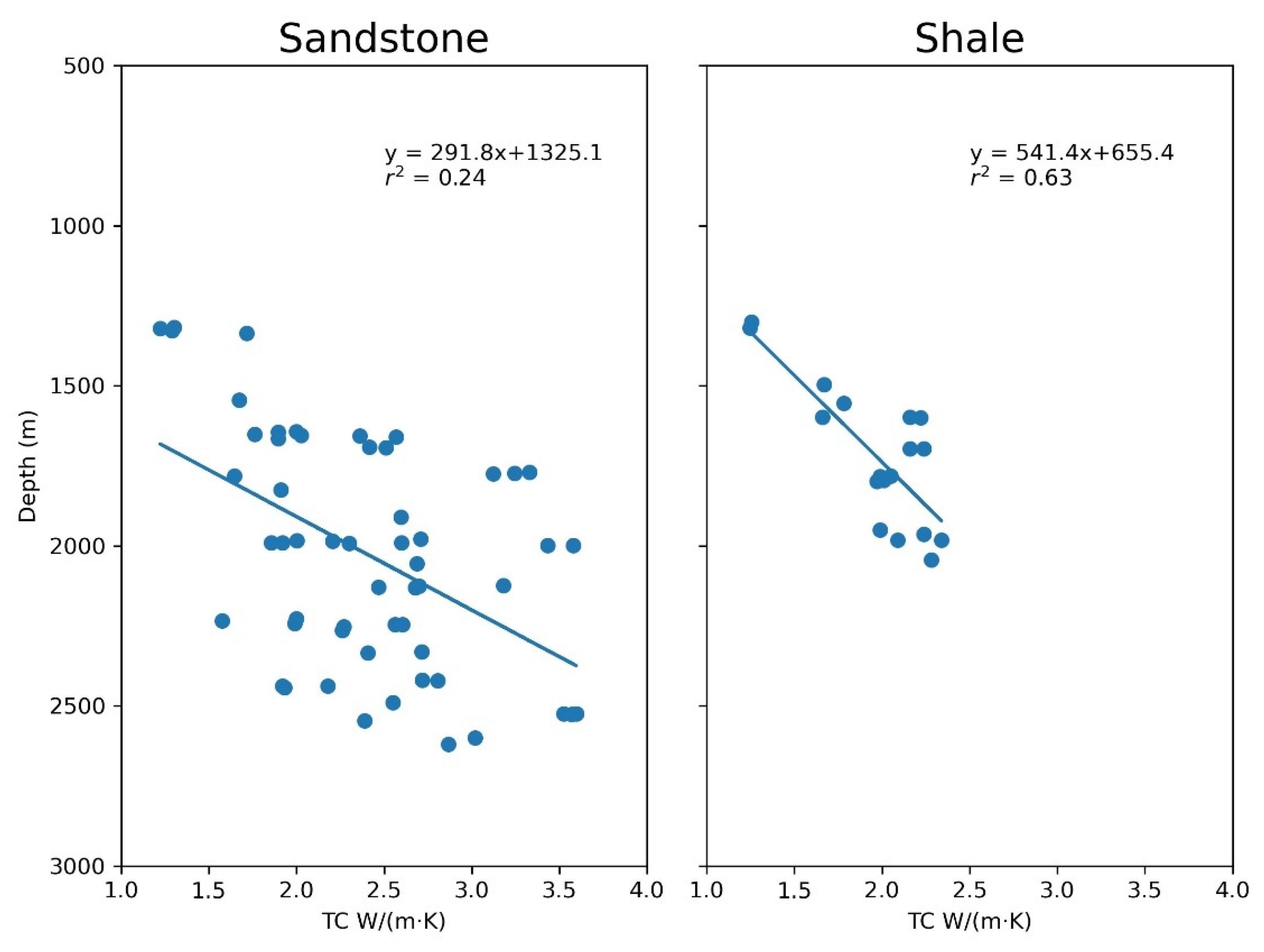
4.1. Laboratory Test TC

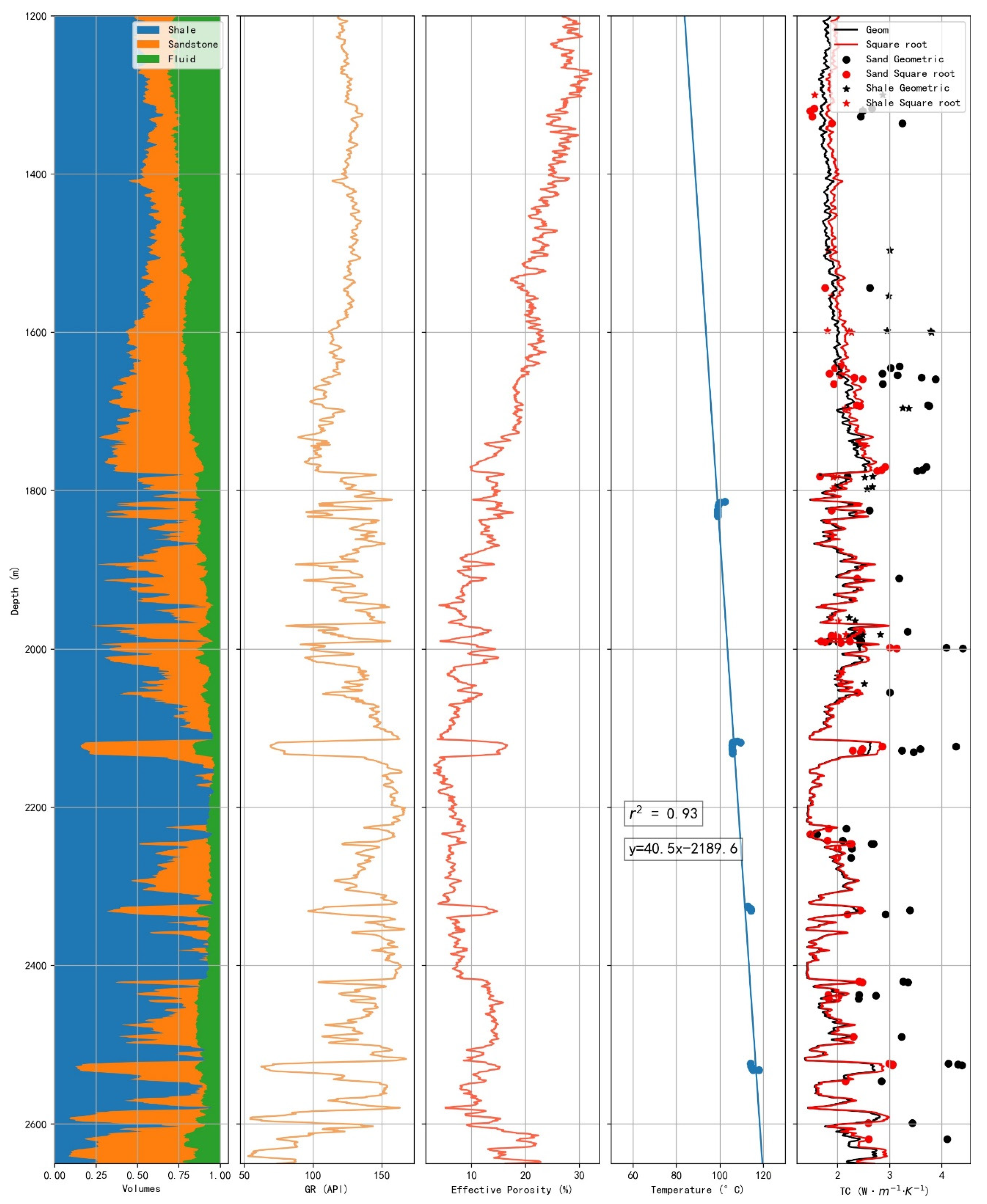
The oil company did not obtain enough samples from one well, so the samples used in this paper are the mixed ones obtained from a closed well in the same stratum. The depth was the buried depth below the seabed. The number of sandstone samples was much more than that of the shale because the oil company has more interest in the sandstone, which is more likely to have oil reservoirs.

Figure 1 shows the TC measurement results for the sand and the shale with the Gauss distribution. It shall be noted that the sand and the shale were identified by eye inspection. There was no clear boundary between the sand and the shale. The median value was “the middle value” in a data set and could also reflect the average value of the data set. It was called “robust against outliers”, whereas the mean value was “sensitive to outliers”. In this study, the mean and the median values were remarkably close to each other in the sandstone and the shale. Therefore, the testing method was reliable, and the results could faithfully represent the TC values of the bore samples. The TC value of the sandstone was in the range from 1.22 to 3.6 $\mathrm{W}·{\mathrm{m}}^{-1}·{\mathrm{K}}^{-1}$ with a mean value of 2.4 ± 0.61 $\mathrm{W}·{\mathrm{m}}^{-1}·{\mathrm{K}}^{-1}$. The TC value of the shale was in the range from 1.25 to 2.34 $\mathrm{W}·{\mathrm{m}}^{-1}·{\mathrm{K}}^{-1}$ with a mean value of 1.96 ± 0.32. The TC value of the sandstone (~2.4) was larger than that of the shale (1.96). The lithology played a key role in this TC value difference. However, the TC value of the shale is more centralized than that of the sandstone. Both the TC values of the sandstone and the shale increased with the increase in the depth, as shown in Figure 2. The correlation coefficient of the shale was 0.63, which was larger than that of the sandstone (0.24). This was due to the larger compaction coefficient of the shale.

4.2. Predicted TC

The left-most figure in Figure 3 shows the volume model of the rock. The volume of the shale was changeable but had an increasing trend along with the depth. The upper part (1200–1600 m) was somewhat uniform and the TC value increased monotonously along with the depth. However, the lower part (1600–2650 m) was sand–shale interbeds and the TC value changed along with the change in the lithology. The porosity ranged from 5% to 33% and was decreasing with the increase in the depth, which should be caused by compaction. As is shown in the right-most figure in Figure 3, the geometric mean value was smaller than the square root mean value. The difference was larger in the “sand” segment and smaller in the “shale” segment. It seems that the small values had higher weights in the geometric mean model. In all, lithology was still the key in controlling the TC of rocks. The geometric mean looks inappropriate when inversely calculating the TC value of the solid, which was more than 20 W/(m·K) and was much higher than that of the pure quartz (7.5 W/(m·K)). The very low TC value of the air ($2.6\times {10}^{-2}$ W/(m·K)) should be the reason for this high TC value of the solid. The square root model seems to be reasonable, so the following discussion is based on the square root model.

5. Discussion

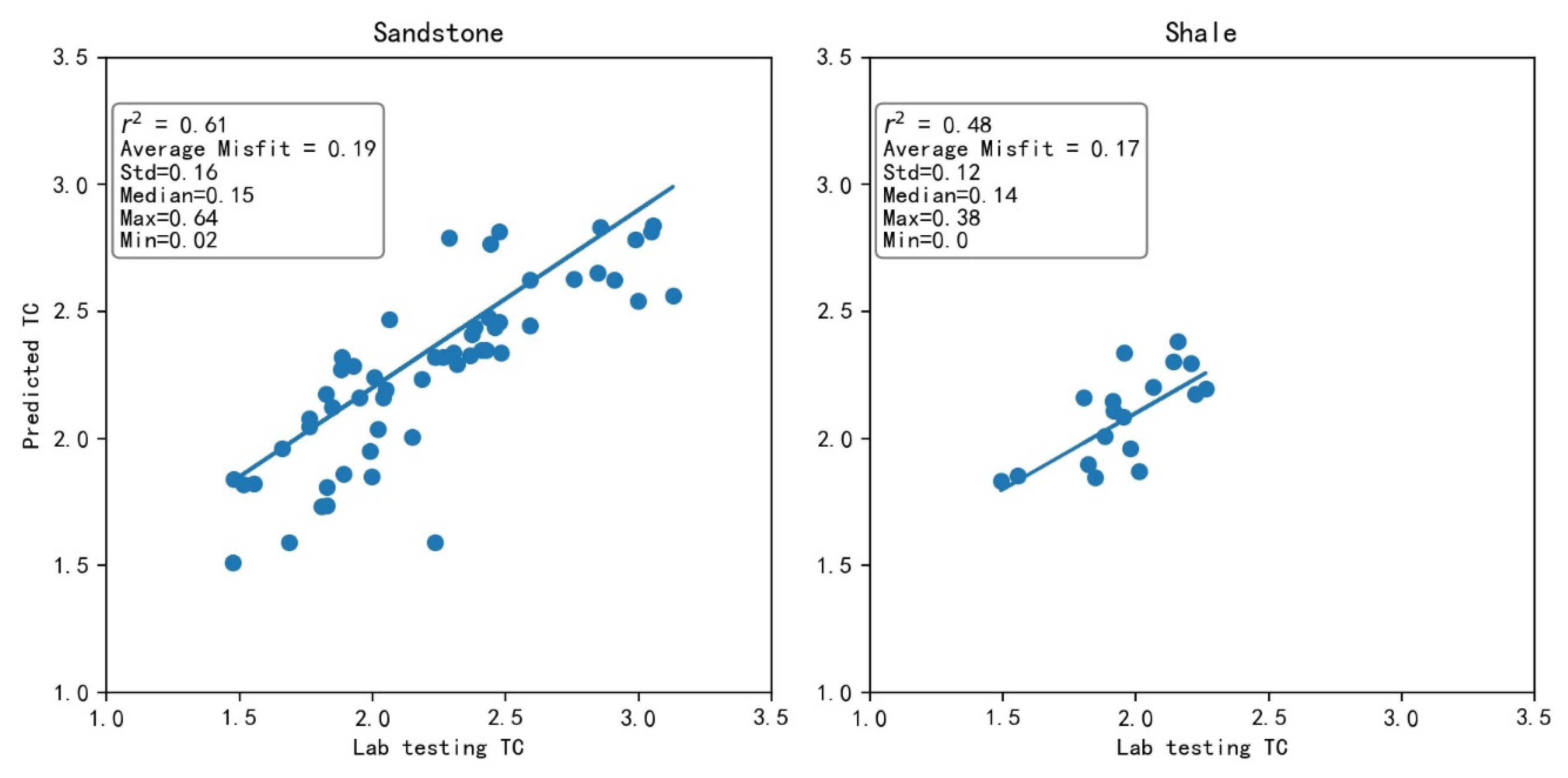
5.1. Comparison between Predicted TC and Test TC

Before comparing with the predicted TC values obtained from the well logging, the laboratory testing TC values should be corrected to in situ TC values. The laboratory testing TC was obtained by using dry samples which were considered to be the mixture of the solid and the air. Therefore, we should use the mixing law to inversely calculate the TC value of the solid first. We were not allowed to take away the core samples to test their porosity by the oil company, so effective porosity from well logs was used here. The next stages were the same as procedures 3 and 4 in estimating the TC value from the well logs.

We used the r-square and the average misfit to describe the degree of the fitness as given by:

$$Misfi{t}_{average}=mean\left(\left|T{C}_{predicted}^i-T{C}_{lab}^i\right|\right)$$

(11)

where i represents the sample number.

As shown in Figure 4, the average misfit of the sand was 0.19 ± 0.16 W/(m·K), with about 8% relative error. The r-square was 0.61, indicating a good but not so excellent model prediction. For the shale, the average misfit was smaller (0.17 ± 0.12 W/(m·K), ~7% relative error), but the r-square (0.48) was not good. This could have resulted from the limited number of samples. The span of the misfit is large in both sandstone (0.2–0.64) and shale (0.0–0.38). Therefore, there could be some outliers in the misfits, which could come from other effects (e.g., oil or gas filling, pressure). Meanwhile, TC is anisotropic, and the observed TC was scanned along the vertical direction representing the horizontal TC. This also led to errors. More studies on the same well at the same depth should be carried out in the future. In general, there was a good agreement between the predicted TC values and the laboratory testing TC values.

The biggest challenge of the comparison between predicted TC and test TC is depth matching. Compared to the well logs, the core samples have lower depth resolution, so the same depth reads from well logs and the core might mean different true depths, which could lead to significant error in sand–shale interbeds. Estimating porosity is another difficulty, and well log data interpretation needs experience, more data (other well logs, cuttings, and mud logging), and professional software to process and interpret well logging data. Thus, a well interpreted porosity from an oil company should do a favor in fitting the test TC. Further, we only consider the situation that the fluid is water. However, in the oil field, it could be oil, gas, water, or a mix of them. The gas (0.026 W/(m·K)) and oil (0.14 W/(m·K)) can largely decrease the TC of rock, and cause an abnormally high gradient [22]. Meanwhile, gas filling increases the pressure of the fluid and decreases the pressure of the rock matrix, so the pressure effect of TC could be taken into account. Although the model is not perfect, the predicted TCs are in agreement with the test TCs in larger numbers.

5.2. Application to Geothermal Energy

Geothermal energy is the heat coming from the sub-surface of the earth [24]. It is one of the cleanest forms of energy, and geothermal resources occur where the heat flow is high, allowing energy to be exploited economically for electricity generation or direct use [25,26]. High-temperature geothermal energy is used to generate electricity [27], while low-temperature geothermal energy is like a thermal battery for heating and cooling buildings and other uses [28]. Furthermore, geothermal energy is stable and can provide 24-h-a-day base load without mega-sized energy storage systems, so it has significant potential in future national renewable energy markets [29,30]. The demand for renewable energy is growing strongly in the coming decade [29]. The global geothermal capacity in 2020 was 14 GW, and it is still growing [31]. At present, atmospheric carbon dioxide and climate change are a great challenge for human beings [32]. Geothermal energy and other renewable energy are the keys to solve this problem [25,33].

TC plays a key role in geothermal energy study, and geothermal energy is a clean, stable, and renewable energy source [4,34]. Firstly, heat flow can be estimated by Q = G × TC (Q is heat flow, G is gradient). Heat flow is the primary constraint on Earth’s heat engine, whose nature and history govern the planet’s thermal, mechanical, and chemical evolution [35]. Additionally, heat flow can be a good indicator to investigate the tectonic background and lithosphere thermal structure. After we obtain enough heat flow data, we can figure out a heat flow contour map, which can help us to find a good geothermal target area [36]. Besides, TC can be used in calculating the temperature distribution (temperature of the geothermal reservoir). Based on the temperature field and other reservoir parameters (heat capacity, porosity, surface temperature, etc.), we can use the volumetric method which is simple and convenient to estimate the geothermal energy resource [37,38].

This model is a good choice for oil fields (especially old oil fields) to estimate geothermal energy. The abandoned wells in oil fields have good and well interoperated well log data. After oil and gas exploitation, the fluid is mainly water, which means less abnormal TC. Using those data, the TC can be determined by our model. Given the predicted TC and temperature logs in enough wells, we can obtain the heat flow contour map, which can imply the thermal anomaly area. If we find the geothermal energy reservoir, TC is used to estimate the temperature field and the geothermal energy resource. With knowing the geothermal energy resource, the oil field can draft an exploitation strategy. Additionally, the exploitation of geothermal energy is remarkably similar with that of oil and natural gas [39]. Without drilling special wells, geothermal resources can bring huge economic and environmental benefits [40,41].

6. Conclusions

In this research, the following conclusions were obtained.

We have proposed a method to predict TC based on the square root model and well logs (GR, neutron porosity, temperature), and the predicted TC values showed good fitting with the laboratory TC values.

The proposed model works better in predicting the TC of sandstone.

This model could be used to calculate the TC in boreholes without core samples in the oil field. With the TC, we can determine the heat flow and estimate the geothermal energy.

References

1. Beardsmore, G.R.; Cull, J.P. Crustal Heat Flow: A Guide to Measurement and Modelling; Cambridge University Press: Cambridge, UK, 2001. [Google Scholar]
2. Goss, R.; Combs, J.; Timur, A. Prediction of Thermal Conductivity in Rocks from other Physical Parameters and from Standard Geophysical Well Logs. In Proceedings of the SPWLA 16th Annual Logging Symposium, New Orleans, LA, USA, 4 June 1975. [Google Scholar]
3. Ellabban, O.; Abu-Rub, H.; Blaabjerg, F. Renewable energy resources: Current status, future prospects and their enabling technology. Renew. Sustain. Energy Rev. 2014, 39, 748–764. [Google Scholar] [CrossRef]
4. Olasolo, P.; Juárez, M.C.; Morales, M.P.; D’Amico, S.; Liarte, I.A. Enhanced geothermal systems (EGS): A review. Renew. Sustain. Energy Rev. 2016, 56, 133–144. [Google Scholar] [CrossRef]
5. Cermak, V.; Rybach, L. Terrestrial Heat Flow and the Lithosphere Structure; Springer Science & Business Media: New York, NY, USA, 2012. [Google Scholar]
6. Jiang, G.Z.; Gao, P.; Rao, S.; Zhang, L.Y.; Tang, X.Y.; Huang, F.; Zhao, P.; Pang, H.; He, L.J.; Hu, S.B.; et al. Compilation of heat flow data in the continental area of China (4th edition). Chin. J. Geophys. 2016, 59, 2892–2910. [Google Scholar]
7. Wang, Z.; Jiang, G.; Zhang, C.; Tang, X.; Hu, S. Estimating geothermal resources in Bohai Bay Basin, eastern China, using Monte Carlo simulation. Environ. Earth Sci. 2019, 78, 355. [Google Scholar] [CrossRef]
8. Pribnow, D.; Williams, C.F.; Sass, J.H.; Keating, R. Thermal conductivity of water-saturated rocks from the KTB Pilot Hole at temperatures of 25 to 300 °C. Geophys. Res. Lett. 1996, 23, 391–394. [Google Scholar] [CrossRef]
9. Wang, Y.; Hu, S.; Wang, Z.; Jiang, G.; Hu, D.; Zhang, K.; Gao, P.; Hu, J.; Zhang, T. Heat flow, heat production, thermal structure and its tectonic implication of the southern Tan-Lu Fault Zone, East–Central China. Geothermics 2019, 82, 254–266. [Google Scholar] [CrossRef]
10. Sun, Q. Analyses of the factors influencing sandstone thermal conductivity. Acta Geodyn. Geomater. 2017, 14, 173–180. [Google Scholar] [CrossRef] [Green Version]
11. Roy, R.; Beck, A. Ihermophysical Properties of Rocks, Physical Properties of Rocks and Minerals; CINDAS Data Series on Material Properties; Touloukian, Y.S., Judd, W.R., Roy, R.F., Eds.; McGraw-Hill: New York, NY, USA, 1981; pp. 409–502. [Google Scholar]
12. Sekiguchi, K. A method for determining terrestrial heat flow in oil basinal areas. Tectonophysics 1984, 103, 67–79. [Google Scholar] [CrossRef]
13. Dixon, J.C. Appendix C, Properties of Water, The Shock Absorber Handbook; John Wiley & Sons: Hoboken, NJ, USA, 2008. [Google Scholar]
14. Popov, Y.; Beardsmore, G.; Clauser, C.; Roy, S. ISRM suggested methods for determining thermal properties of rocks from laboratory tests at atmospheric pressure. Rock Mech. Rock Eng. 2016, 49, 4179–4207. [Google Scholar] [CrossRef]
15. He, L.; Hu, S.; Huang, S.; Yang, W.; Wang, J.; Yuan, Y.; Yang, S. Heat flow study at the Chinese Continental Scientific Drilling site: Borehole temperature, thermal conductivity, and radiogenic heat production. J. Geophys. Res. 2008, 113. [Google Scholar] [CrossRef] [Green Version]
16. Popov, Y.; Bayuk, I.O.; Parshin, A.; Miklashevskiy, D.; Novikov, S.; Chekhonin, E. New Methods and Instruments for Determination of Reservoir Thermal Properties. In Proceedings of the 37th Workshop on Geothermal Reservoir Engineering, Stanford, CA, USA, 30 January–1 February 2012. [Google Scholar]
17. Wang, Y.; Wang, L.; Hu, D.; Guan, J.; Bai, Y.; Wang, Z.; Jiang, G.; Hu, J.; Tang, B.; Zhu, C.; et al. The present-day geothermal regime of the North Jiangsu Basin, East China. Geothermics 2020, 88, 101829. [Google Scholar] [CrossRef]
18. Asquith, G.B.; Krygowski, D.; Gibson, C.R. Basic Well Log Analysis; American Association of Petroleum Geologists Tulsa: Tulsa, OK, USA, 2004; Volume 16. [Google Scholar]
19. Atlas, D. Log Interpretation Charts: Dresser Atlas; Dresser Industries. Inc.: Addison, TX, USA, 1979; 107p. [Google Scholar]
20. Timur, A. An Investigation of Permeability, Porosity, and Residual Water Saturation Relationships. In Proceedings of the SPWLA 9th Annual Logging Symposium, New Orleans, LA, USA, 23 June 1968. [Google Scholar]
21. Glover, P. Petrophysics MSc Course Notes; University of Leeds: Leeds, UK, 2000. [Google Scholar]
22. Schön, J.H. Physical Properties of Rocks: Fundamentals and Principles of Petrophysics; Elsevier: Amsterdam, The Netherlands, 2015; Volume 65. [Google Scholar]
23. Clauser, C. Geothermal energy. In Landolt-Bo¨rnstein Numerical Data and Functional Relationships in Science and Technology, New Series, Group VIII; von Heinloth, K., Ed.; Springer: Berlin/Heidelberg, Germany, 2006; Volume 3. [Google Scholar]
24. Dickson, M.H.; Fanelli, M. Geothermal Energy: Utilization and Technology; Routledge: London, UK, 2013. [Google Scholar]
25. Letcher, T.M. Introduction with a focus on atmospheric carbon dioxide and climate change. In Future Energy; Elsevier: Amsterdam, The Netherlands, 2020; pp. 3–17. [Google Scholar]
26. DiPippo, R.; Renner, J.L. Geothermal energy. In Future Energy; Elsevier: Amsterdam, The Netherlands, 2014; pp. 471–492. [Google Scholar]
27. Barasa Kabeyi, M.J. Geothermal electricity generation, challenges, opportunities and recommendations. Int. J. Adv. Sci. Res. Eng. 2019, 5, 53–95. [Google Scholar] [CrossRef]
28. Phetteplace, G. Geothermal heat pumps. J. Energy Eng. 2007, 133, 32–38. [Google Scholar] [CrossRef]
29. Teske, S.; Fattal, A.; Lins, C.; Hullin, M.; Williamson, L.E. Renewables Global Futures Report: Great Debates towards 100% Renewable Energy; Global Forum of Sustainable Energy: Wien, Austria, 2017. [Google Scholar]
30. Tester, J.W.; Anderson, B.J.; Batchelor, A.S.; Blackwell, D.D.; DiPippo, R.; Drake, E.M.; Garnish, J.; Livesay, B.; Moore, M.C.; Nichols, K.; et al. Impact of enhanced geothermal systems on US energy supply in the twenty-first century. Philos. Trans. R. Soc. A Math. Phys. Eng. Sci. 2007, 365, 1057–1094. [Google Scholar] [CrossRef]
31. IRENA. Renewable Capacity Statistics 2021; The International Renewable Energy Agency: Abu Dhabi, United Arab Emirates, 2021. [Google Scholar]
32. Biron, M. An overview of sustainability and plastics: A multifaceted, relative, and scalable concept. In A Practical Guide to Plastics Sustainability; William Andrew: London, UK, 2020; pp. 1–43. [Google Scholar]
33. Archer, R. Geothermal energy. In Future Energy; Elsevier: Amsterdam, The Netherlands, 2020; pp. 431–445. [Google Scholar]
34. Lu, S.-M. A global review of enhanced geothermal system (EGS). Renew. Sustain. Energy Rev. 2018, 81, 2902–2921. [Google Scholar] [CrossRef]
35. Pollack, H.N.; Hurter, S.J.; Johnson, J.R. Heat flow from the Earth’s interior: Analysis of the global data set. Rev. Geophys. 1993, 31, 267–280. [Google Scholar] [CrossRef]
36. Jiang, G.; Hu, S.; Shi, Y.; Zhang, C.; Wang, Z.; Hu, D. Terrestrial heat flow of continental China: Updated dataset and tectonic implications. Tectonophysics 2019, 753, 36–48. [Google Scholar] [CrossRef]
37. Williams, C.F.; Reed, M.; Mariner, R.H. A Review of Methods Applied by the US Geological Survey in the Assessment if Identified Geothermal Resources; CiteSeer: Princeton, NJ, USA, 2008. [Google Scholar]
38. Zhang, C.; Jiang, G.; Shi, Y.; Wang, Z.; Wang, Y.; Li, S.; Jia, X.; Hu, S. Terrestrial heat flow and crustal thermal structure of the Gonghe-Guide area, northeastern Qinghai-Tibetan plateau. Geothermics 2018, 72, 182–192. [Google Scholar] [CrossRef]
39. Tester, J.W.; Anderson, B.J.; Batchelor, A.S.; Blackwell, D.D.; DiPippo, R.; Drake, E.M.; Garnish, J.; Livesay, B.; Moore, M.C.; Nichols, K.; et al. The Future of Geothermal Energy; Massachusetts Institute of Technology: Cambridge, MA, USA, 2006; p. 358. [Google Scholar]
40. Wang, J.; Qiu, N.; Hu, S.; He, L. Advancement and developmental trend in the geothermics of oil fields in China. Earth Sci. Front. 2017, 24, 1–12. [Google Scholar]
41. Fridleifsson, I.B. Geothermal energy for the benefit of the people. Renew. Sustain. Energy Rev. 2001, 5, 299–312. [Google Scholar] [CrossRef] [Green Version]
Figure 1. Thermal conductivity histograms obtained from the laboratory testing, note that the frequency has been normalized.
Mathematics 09 01176 g001
Figure 2. Relationship between the thermal conductivity and the depth.
Mathematics 09 01176 g002
Figure 3. Results of the sand–shale–water model. Input data: GR—natural gamma-ray, effective porosity, and temperature. Output data: the volume model and the predicted TC.
Mathematics 09 01176 g003
Figure 4. Relationship between the measured TC values and the predicted TC values.
Mathematics 09 01176 g004