An Adaptive Cuckoo Search-Based Optimization Model for Addressing Cyber-Physical Security Problems

Abstract

One of the key challenges in cyber-physical systems (CPS) is the dynamic fitting of data sources under multivariate or mixture distribution models to determine abnormalities. Equations of the models have been statistically characterized as nonlinear and non-Gaussian ones, where data have high variations between normal and suspicious data distributions. To address nonlinear equations of these distributions, a cuckoo search algorithm is employed. In this paper, the cuckoo search algorithm is effectively improved with a novel strategy, known as a convergence speed strategy, to accelerate the convergence speed in the direction of the optimal solution for achieving better outcomes in a small number of iterations when solving systems of nonlinear equations. The proposed algorithm is named an improved cuckoo search algorithm (ICSA), which accelerates the convergence speed by improving the fitness values of function evaluations compared to the existing algorithms. To assess the efficacy of ICSA, 34 common nonlinear equations that fit the nature of cybersecurity models are adopted to show if ICSA can reach better outcomes with high convergence speed or not. ICSA has been compared with several well-known, well-established optimization algorithms, such as the slime mould optimizer, salp swarm, cuckoo search, marine predators, bat, and flower pollination algorithms. Experimental outcomes have revealed that ICSA is superior to the other in terms of the convergence speed and final accuracy, and this makes a promising alternative to the existing algorithm.

1. Introduction

With the norm of cyber-physical systems (CPS), cyber defense systems such as intrusion detection and threat intelligence, which deal with data sources under the constraints of nonnormality and nonlinearity, should be designed to handle these constraints and produce accurate outcomes [1,2]. These models have been developed using nonlinear equation systems (NESs) [3], which need to be accurately solved in reasonable time [4]. Therefore, to overcome NESs, several numerical methods, including the Newton-type method [5] and the iterative and recursive methods [6], have been proposed. However, most of those methods cannot estimate the roots of NESs with a complex nature due to their sensitivity to picking the initial guess of the solutions, which significantly affects the obtained outcomes and stability of those methods [4]. Therefore, the only way to overcome those drawbacks and to estimate the optimal roots is to use evolutionary and meta-heuristic algorithms, which have gained significant attention over the last decades due to their superiority in terms of local minima avoidance, convergence speed, and reaching the optimal solution in a reasonable time.

The evolutionary algorithms (EAs) and swarm algorithms (SAs) have achieved significant achievements in real-world optimization problems [7,8,9,10,11,12,13,14,15,16,17,18], particularly the convex, discontinuous nonlinear optimization problem [11,19,20]. Therefore, they have been widely used in the literature for solving the NESs. Unfortunately, the existing algorithms still suffer from local minima and convergence speed to the optimal root. This causes two problems when solving NESs: (1) consuming several numbers of function evaluations before reaching the optimal root in some cases, and (2) the algorithms are unable to find the optimal root with an increasing number of function evaluations due to the weak ability of the algorithms in exploring as much of the search space as possible while avoiding getting stuck in local minima problems. In cybersecurity, data distributions of intrusion detection and threat models often demand nonlinear and non-Gaussian systems that can discriminate small variations between normal and suspicious behaviors [21]. In this paper, the cuckoo search algorithm (CSA) is improved in an effective way to help it avoid those two problems while solving NESs. The algorithm is named as the improved CSA (ICSA). ICSA was extensively validated using 34 well-known NES cases and compared with some recently published, well-established optimization algorithms, namely the slime mould algorithm (SMA, 2020) [22], marine predators algorithm (MPA, 2020) [23], Bat algorithm (BA, 2012) [24], salp swarm algorithm (SSA, 2017) [25], standard cuckoo search algorithm (CSA, 2009) [26], and flower pollination algorithm (FPA, 2012) [27], under various statistical analyses that can flexibly fit nonlinear distributions of CPS-driven data sources, efficiently enhancing the discovery of anomalous events. The experiments show that our improved algorithm has significant performance for most test cases concerning the convergence speed and final accuracy in comparison to the abovementioned algorithms. The main contributions in this research are as follows:

(a)

Improving the classical CSA using an effective strategy called the convergence improvement strategy (CIS) to produce a new variant able to accurately tackle NESs. This variant was named ICSA.

(b)

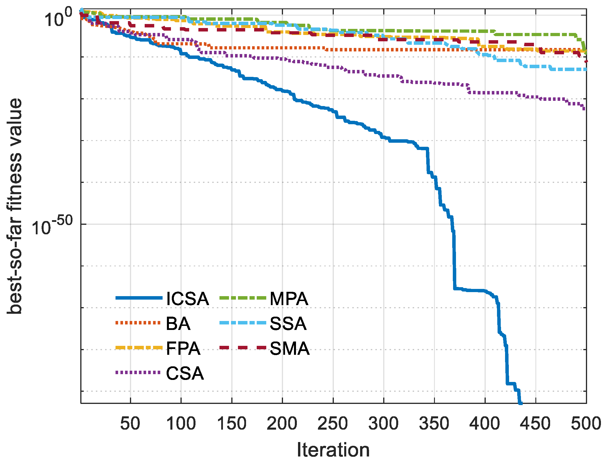
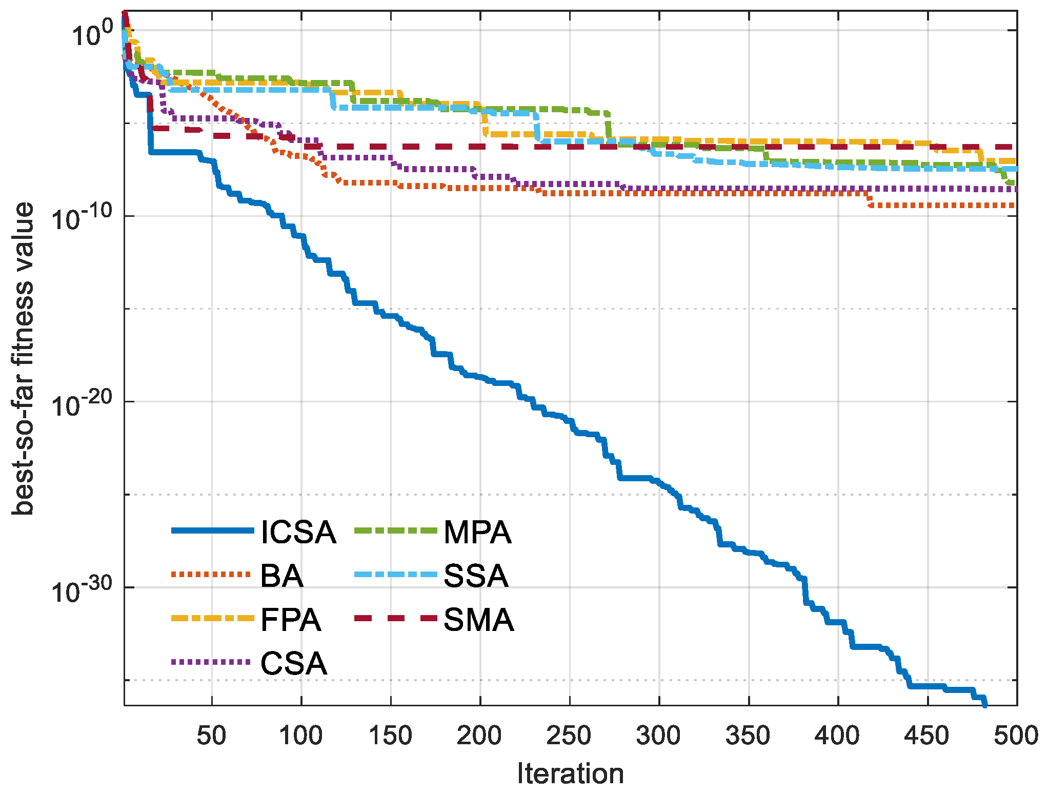
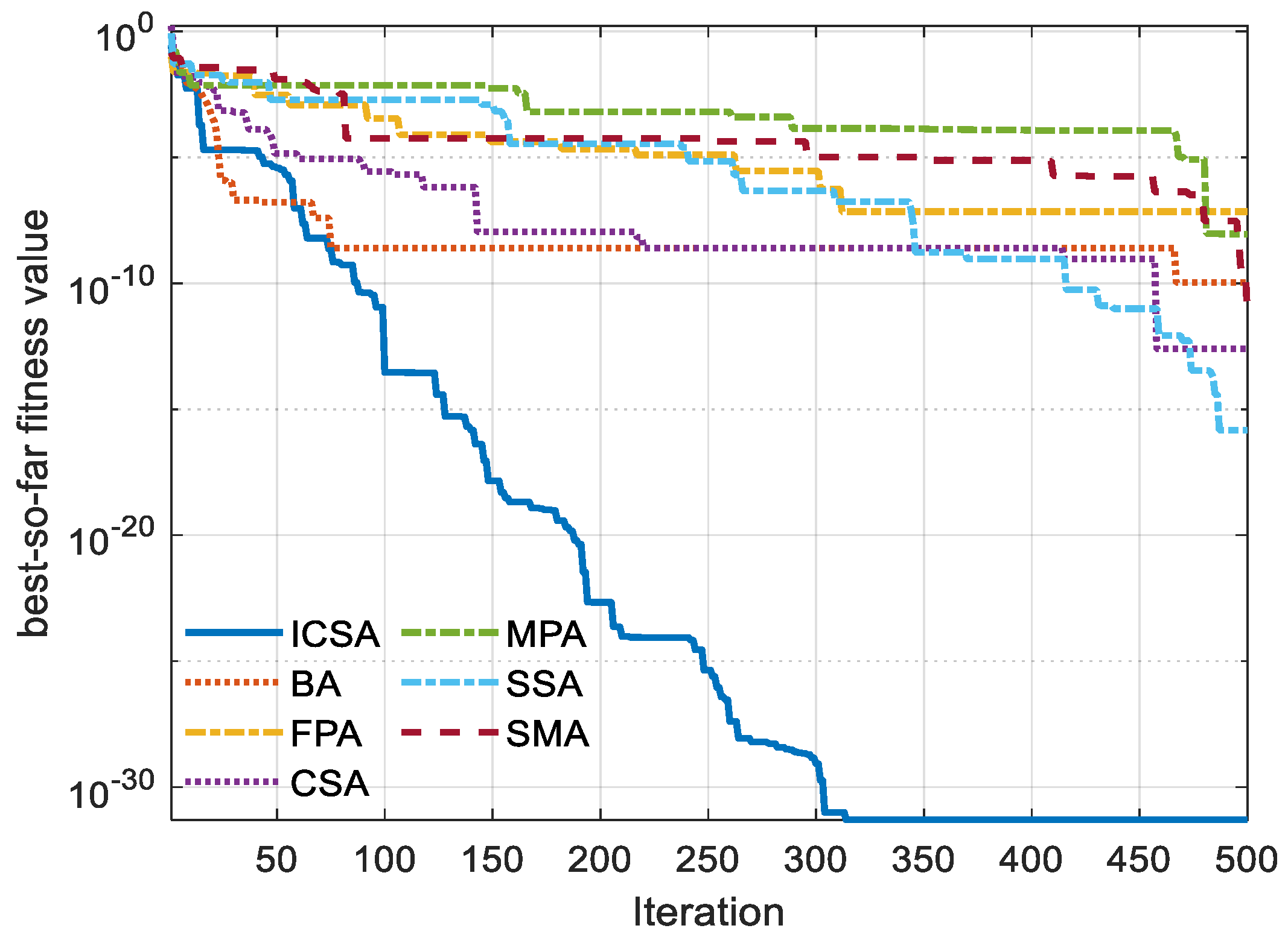
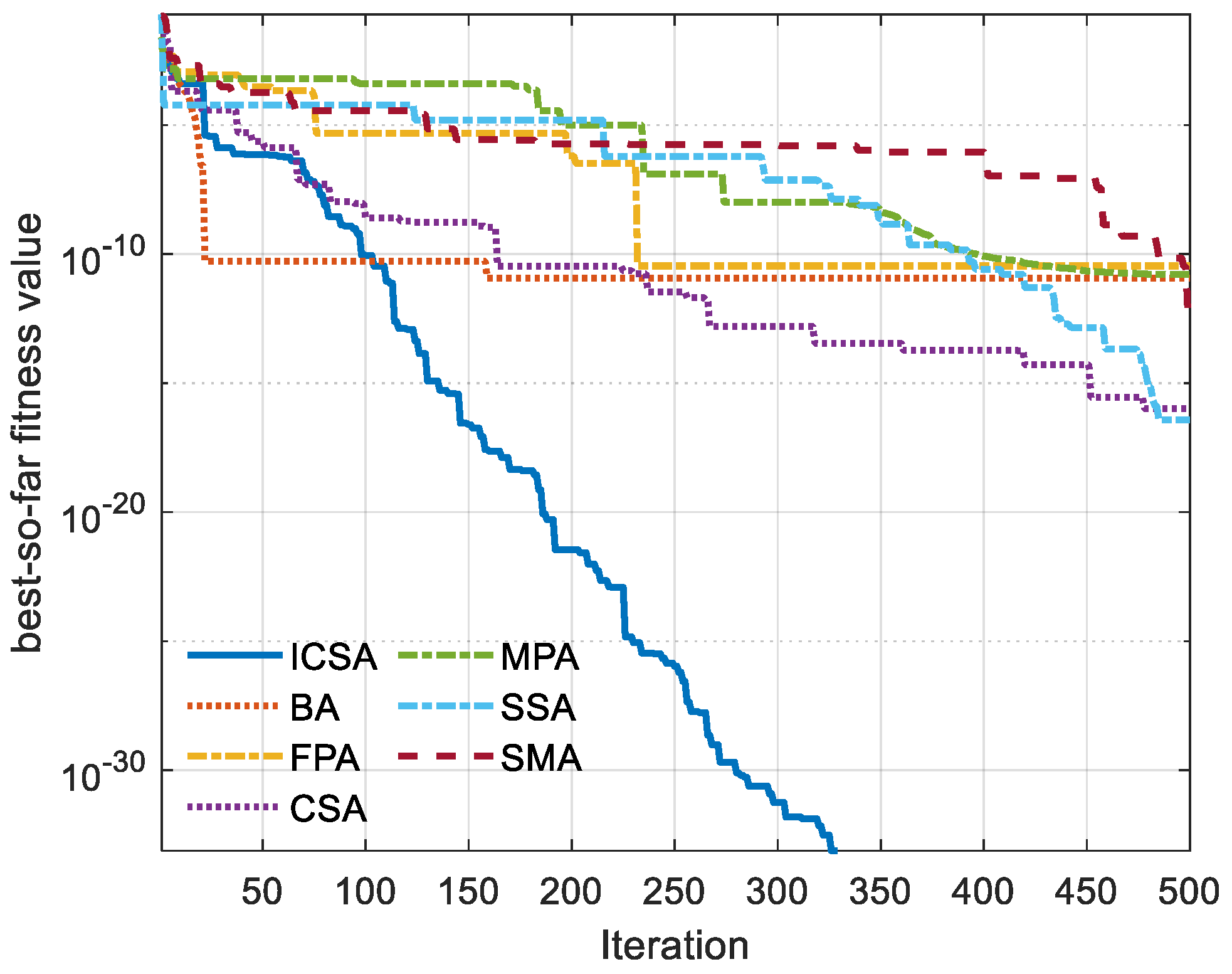
The experiments conducted on 34 well-known NES cases to assess the performance of this variant, in addition to comparing its performance with 6 well-established optimization algorithms, show the efficacy of this variant in terms of the convergence speed and final accuracy for most test cases.

The remainder of this paper is organized as follows: Section 2 presents the literature review, Section 3 overviews the standard CSA, Section 4 extensively describes our proposed work, and Section 5 shows our experimental outcomes and some discussions. Finally, Section 6 shows some conclusions devised from our proposed work and discusses our future work.

2. Literature Review

This section is divided into two parts. The first part will define the problem formulation of the NES, and the second reviews the EAs and the SAs proposed in the literature to tackle the NESs.

2.1. Problem Description

Generally, nonlinear equation systems are mathematically formulated as follows:

$$S\left(x\right)=\{\begin{array}{c}{f}_1\left(x_1, x_2, x_3,\dots \dots \dots , x_d\right)=0\\ f_2\left(x_1, x_2, x_3,\dots \dots \dots , x_d\right)=0\\ f_3\left(x_1, x_2, x_3,\dots \dots \dots , x_d\right)=0\\ .\\ .\\ .\\ f_n\left(x_1, x_2, x_3,\dots \dots \dots , x_d\right)=0\end{array}$$

(1)

where $d$ denotes the number of decision variables of the equation; $n$ refers to the number of equations; $x$ is a vector of $d$-dimensions and includes a solution to the NES, where each dimension within this solution must be subject to its search boundary: lower bound (Lb) and upper bound (Ub).

As formulated in Equation (1), x denotes the decision variables and the attributes/features in a cyber-physical problem, specifically, a machine learning-based intrusion detection. When these attributes were statistically evaluated using the Kolmogorov–Smirnov (K–S) test, the outcomes revealed that the attributes follow nonlinear and non-Gaussian distributions. This indicates that the models must employ nonlinear equations to perfectly fit small variations of normal and anomalous behaviors [1].

To solve the nonlinear attributes/decision attributes of NESs in a machine learning-based intrusion detection problem, Equation (1) comprises n equations, while the optimization algorithms usually work to minimize only one. Therefore, Equation (1), which defines the NESs, was transformed into Equation (2) to become a minimization problem that could be solved using an optimization algorithm.

$$f\left(x\right)={\displaystyle {\displaystyle \sum }_{i=1}^n}{f}_i^2\left(x\right)$$

(2)

This equation is considered as the objective function that needs to be minimized using optimization techniques to find the optimal roots and clear boundaries between the nonlinear attributes of normal and suspicious events.

2.2. Swarm and Evolutionary Algorithms

In [28], the social emotion optimization algorithm (EOA) was integrated with a metropolis rule as an attempt to escape the local minima that has been proposed for the NESs. This hybrid algorithm, abbreviated as MSEOA, was compared with the particle swarm algorithm (PSO) and the standard EOA to determine the best one for solving four nonlinear equations. In the experiments, MSEOA was found to be more effective for solving the NESs. Further, Wu Z. and L. Kang [29] proposed a parallel Elite-subspace evolutionary algorithm (PESEA) to solve the NESs in a reasonable time. PESEA was validated using five nonlinear equations to determine its punctuality in estimating their optimal roots. Based on the conducted experiments, PESEA is faster and more punctual.

To solve NESs, the authors of [30] suggested a hybrid approach that involved using the capability of chaos maps to dramatically explore the search space with a quasi-Newton method outstanding with high convergence. The authors of [31] integrated an evolutionary algorithm with additional strategies. The authors combined the k-means clustering method with niching to guide the optimization process to the multiple roots within the search space, and avoided getting stuck in local minima using the two methods. Finally, the authors proposed using various crowding factors to decrease the replacement error for finding the multiple roots of the NESs, and this algorithm was called a one-step k-means clustering-based differential evolution (KSDE). Following the development of KSDE, 30 problems have been used to validate its performance, in addition to comparing the algorithm with some of the state-of-the-art methods to show its superiority.

Rizk-Allah [32] proposed a new approach, namely Q-SCA, to solve NESs based on modifying the sine-cosine algorithm (SCA). Using Q-SCA, the Rizk-Allah dynamically adjusted the SCA’s search ability to search around the current location or the best-so-far solution to improve its exploitation capability as an attempt to accelerate the local convergence rate. Q-SCA also used the quantum local search (QLS) to improve the obtained solutions as an attempt to balance the algorithm’s exploration and exploitation capability. This approach was investigated among 12 NESs and 2 electrical applications and compared with several algorithms to show its stability and accuracy in achieving true better outcomes. The experimental outcomes showed the superiority of this algorithm over the standard one. The authors of [33,34,35] adapted various genetic algorithms (GAs) to solve the NESs.

The grasshopper optimization algorithm (GOA) [36] has been hybridized with the GA to produce a new hybrid algorithm known as hybrid GOA with GA for solving the NESs. This hybrid algorithm combined the merits of both GA and GOA to escape from the local minima and accelerate the convergence speed. More than that, the grey wolf optimizer (GWO) has been integrated with differential evolution to tackle the NESs; this algorithm was named GWO-DE. In [37], differential evolution improved and integrated with a restart strategy, namely DE-R, has been proposed for the NESs. DE-R used a new mutation operator and a restart technique to promote the exploration ability and avoid getting stuck into local minima. DE-R was compared with some recently developed algorithms over a set of nonlinear equation systems and real-world problems to show the effectiveness of DE-R.

Ultimately, several continuous evolutionary and swarm intelligence algorithms have been promoted that might be applied to tackle this problem in the future in the hope of finding better outcomes; some of those algorithms are natural evolution strategies [38], particle swarm optimization in the estimation of distribution algorithms (EDAs) framework [39], the EDAs [40], and the covariance matrix adaptation evolution strategy [41].

3. Standard Algorithm: Cuckoo Search Algorithm

Xin Shen Yang [26] proposed a new metaheuristic algorithm, namely the cuckoo search algorithm (CSA), for solving optimization problems. Recently, CSA was employed for selecting the most relevant nonlinear attributes and discovering suspicious observations [42]. This research is motivated to develop a new variant of CSA that can efficiently deal with nonlinear functions and will be effective in finding the clear bounds of legitimate and suspicious behaviors while implementing classification methods. CSA is inspired by the obligate brood parasitism of some cuckoo birds by laying their eggs in the nests of other host birds. Sometimes, when the cuckoos find out the eggs in their nests do not belong to them, those foreign eggs are either flung out or all the nests are abandoned. In general, the CS algorithm is based on three rules:

(1)

Each cuckoo lays one egg at a time and put its egg in a randomly chosen nest;

(2)

The best nests with eggs having high quality will be used in the next generation;

(3)

The available host nests number is fixed, and the cuckoos can discover a foreign egg with a probability $p_a$ that varies between 0 and 1.

CSA could balance the global random walk and local random walk to promote its searchability for reaching better outcomes. Mathematically, the global random walk is formulated as

$$x_i^{t+1}=x_i^t+\alpha ℒ\left(s,\lambda \right)$$

(3)

where $t$ express the current iteration, $x_i^t$ is the current position of the $i^{th}$ cuckoo, $x_i^{t+1}$ indicates the next position, $ℒ\left(\mathrm{s},\mathsf{\lambda }\right)$ is the levy distributions used to determine the size of the step of random walk,$s$ is the stepsize, and $\alpha$ is a positive scaling factor. The local random walk is defined as follows:

$$x_i^{t+1}=x_i^t+\alpha s⨂H\left(p_a-\epsilon \right)⨂\left(x_j^t-x_k^t\right)$$

(4)

where $⨂$ indicates the entry-wise multiplication operator, $H$ is a heavy-side function, $\epsilon$ is a random number generated based on the normal distribution, and $x_j^t \mathrm{and} x_k^t$ are two random positions chosen randomly from the current population. $t_{\mathit{max}}$ indicates the maximum number of iterations. The steps of CSA are shown in Algorithm 1.

Algorithm 1 The steps of CSA

Create an initial population of N solutions. Initialize $\alpha$, $p_a$, and $t=0;$ Evaluate the fitness for each solution and determine the best-so-far solution $x^{*}$. while (t < $t_{max}$) Create a new population using Equation (3) and insert better ones into the current population. t = t + 1; Create a new population using Equation (4) and add into the current the best ones. t = t + 1; end while

4. Proposed Algorithm

In this section, the steps of the proposed algorithm, known as an improved cuckoo search algorithm (ICSA), will be clearly described; those steps are initialization, evaluations, and ICSA.

4.1. Initialization

At the outset of the optimization algorithm, a group of N solutions will be created with d dimensions for each, which are randomly initialized within the search space of the problem according to the following equation:

$$\forall \mathrm{i}\in \mathrm{N},{\overrightarrow{x}}_i=\overrightarrow{L}+\overrightarrow{r}⨂(\overrightarrow{U}-\overrightarrow{L})$$

(5)

where $\overrightarrow{U }\mathrm{and}\overrightarrow{L}$ are two vectors including the upper and lower bounds of various problem dimensions, and $\overrightarrow{r}$ is a vector of d elements assigned randomly between 0 and 1. After completing the initialization step, those initial solutions will be evaluated using Equation (2) to determine the quality of each one, and the one with the highest quality will be extracted to help later in improving the quality of the new populations.

4.2. Convergence Improvement Strategy (CIS)

A new strategy, called convergence improvement strategy, is proposed for improving the performance of the meta-heuristic algorithm to achieve better convergence, in addition to improving final accuracy, and enhancing the ability to select the most significant attributes for CPS problems. This strategy is two-fold: the first aspect is based on searching the best-so-far solutions for a better solution using Equation (6) to save time in the optimization process if the near-optimal solution is found around this best-so-far case, but this best-so-far solution also may be a trap to drift the algorithm into local minima, hence reducing the possibility of reaching better outcomes. Therefore, the second aspect, formulated mathematically in Equation (7), is used to avoid falling into local minima based on multiplying the current position in a vector $vc$ generated randomly based on the uniform distribution with the lower endpoints $-1\times r_1$ and upper endpoint $r_1$; where $r_1$ is a value created randomly between 0 and 1.

$$x_i^{t+1}=x^{*}+\alpha ℒ⨂\left(x_i^t-x^{*}\right)$$

(6)

$$x_i^{t+1}=vc⨂x_i^t$$

(7)

The swap between Equations (6) and (7) is determined based on a probability, namely γ, picked during the experiments by the researcher at the expense of their outcomes; this probability in our experiment was set to 0.1, after extensive experiments.

4.3. Improved Cuckoo Search Algorithm (ICSA)

To improve the global random walk of CSA, CIS is called after executing the global random walk, with probability pr to accelerate the convergence speed toward the best-so-far solution, using the first aspect, and to avoid getting stuck into local minima, using the second aspect. Generally, Algorithm 2 elaborates the steps of ICSA after integrating CIS. Before starting the optimization process by ICSA, N solutions will be randomly distributed within the search space to cover it as much as possible, in addition to initializing the main parameters of the ICSA. Then, those solutions will be updated by the global random walk integrated with the CIS with a probability pr set to 0.5, as explained in the experiments section, to promote its searchability for reaching better outcomes, as described in Lines 6–16 in Algorithm 2. In Line 19, the current solution will be updated using the local random walk as an attempt to avoid getting stuck into local minima. This optimization process is continuously running until the termination condition is satisfied (reaching the maximum iteration $t_{max}$).

Algorithm 2 The steps of ICSA

Create an initial population of N solutions. Initialize $\alpha$, $p_a$, γ, and $t=0;$ Evaluate the fitness for each solution and determine the best-so-far solution $x^{*}$. while (t < $t_{max}$) nX: Create a new population using Equation (3) For (i = 1: N) $r$: create a random number between 0 and 1. if (r > pr) $r_1$: create a random number between 0 and 1. if ($r_1$ < $\gamma$) Update the current solution $n{X}_i$ using Equation (6) Else Update the current solution $n{X}_i$ using Equation (7) End if End if End for Evaluate each solution in the new population and insert better ones into the current population. t = t + 1; Create a new population using Equation (4) and add into the current the best ones. t = t + 1; end while

5. Outcomes and Discussion

This section validates the performance of the proposed algorithm, ICSA, to examine its efficacy, in addition to witnessing its superiority compared to some well-established optimization algorithms under various statistical analyses. Best, average (Avg), worst, and standard deviation (SD) were obtained as the fitness values within 30 independent trials, and the Wilcoxon rank-sum test was used to determine significance. The compared algorithms used in our experiments included slime mould algorithm (SMA, 2020) [22], marine predators algorithm (MPA, 2020) [23], Bat algorithm (BA, 2012) [24], salp swarm algorithm (SSA, 2017) [25], standard cuckoo search algorithm (CSA, 2009) [26], and flower pollination algorithm (FPA, 2012) [27]. Algorithms were programmatically implemented using MATLAB R2019a based on the cited parameters under the same operating conditions as the proposed algorithm; those conditions are summarized as the maximum number of iterations, the population size, and the number of independent runs, which are respectively set to 500, 30, and 30. A computer with 32GB of RAM, Intel(R) Core(TM) i7-4700MQ CPU @ 2.40 GHz, and a 64-bit operating system (Windows 10) was used to conduct all the experiments.

To validate the performance of our proposed algorithm, 34 test cases of the nonlinear equation systems used widely in the literature were used. Most of these equations were widely used in the design of cybersecurity models, such as intrusion detection and threat models, to differentiate between small variations of normal and abnormal activities in CPSs. The characteristics of these functions are summarized as the number of dimensions (D), the search space (ℝ) for each dimension, and formulas to those functions, and their references are presented in

Table 1. Descriptions of the nonlinear equation systems used in our experiments.

Function	Formulas	D	$\mathit{ℝ}$	References
F1	$x_1-\sin \left(5\pi x_2\right)=0$ $x_1-x_2=0$	2	$x_i=\left[-1,1\right]\forall i=1, 2$	[43]
F2	$x_1-\cos \left(4\pi x_2\right)=0$ $x_1^2+x_2^2-1=0$	2	$x_i=\left[-10,10\right]\forall i=1, 2$	[43]
F3	$x_1-0.25428722-0.18324757x_4{x}_3{x}_9=0$ $x_2-0.37842197-0.16275449x_1{x}_{10}{x}_6=0$ $x_3-0.27162577-0.16955071x_1{x}_2{x}_{10}=0$ $x_4-0.19807914-0.15585316x_7{x}_1{x}_6=0$ $x_5-0.44166728-0.19950920x_7{x}_6{x}_3=0$ $x_6-0.14654113-0.18922793x_8{x}_5{x}_{10}=0$ $x_7-0.42937161-\mathrm{0..21180486}{x}_2{x}_5{x}_8=0$ $x_8-0.07056438-0.17081208x_1{x}_7{x}_6=0$ $x_9-0.34504906-0.19612740x_{10}{x}_6{x}_8=0$ $x_{10}-0.42651102-\mathrm{0..21466544}{x}_4{x}_8{x}_1=0$	10	$x_i=\left[-10,10\right]\forall i=1, \dots ,10$	[44]
F4	$3.0-x_1{x}_3^2=0$ $x_3\sin \left(\frac{\pi }{x_2}\right)-x_3-x_4=0$ $-x_{2}x3\exp \left(1.0-x_1{x}_3\right)+0.2707=0$ $2x_1^2{x}_3-x_2^4{x}_3-x_2=0$	4	$x_i=\left[0, 5\right]\forall i=1, 4$	[45]
F5	$4x_1^3+4x_1{x}_2+2x_2^2-42x_1-14=0$ $4x_2^3+2x_1^2+4x_1{x}_2-16x_2-22=0$	2	$x_i=\left[-20,20\right]\forall i=1, 2$	[46]
F6	$-\sin \left(x_1\right)\cos \left(x_2\right)-2\cos \left(x_1\right)\sin \left(x_2\right)=0$ $-\cos \left(x_1\right)\sin \left(x_2\right)-2\sin \left(x_1\right)\cos \left(x_2\right)=0$	2	$x_i=\left[0,\pi \right]\forall i=1, 2$	[47]
F7	$x_1^2+x_2^2-1.0=0$ $x_3^2+x_4^2-1.0=0$ $x_5^2+x_6^2-1.0=0$ $x_7^2+x_8^2-1.0=0$ $4.731 · {10}^{-3} x_{1}x3-0.3578x_2{x}_3-0.1238x_1+x_7-1.637 · {10}^{-3}{x}_2-0.9338x_4-0.3571=0$ $0.2238x_1{x}_3+0.7623x_2{x}_3+0.2638x_1-x_7-0.07745x_2-0.6734x_4-0.6022=0$ $x_6{x}_8+0.3578x_1+4.731 · {10}^{-3}{x}_2=0$ $-0.7623x_1+0.2238x_2+0.3461=0$	8	$x_i=\left[-1,1\right]\forall i=1, \dots ,8$	[4]
F8	$x_i-\cos \left(2x_i-{\displaystyle {\displaystyle \sum }_{j=1}^D}{x}_j\right)=0$	3	$x_i=\left[-20,20\right]\forall i=1,\dots , D$	[48]
F9	$x_1^2-x_2-2=0$ $x_1+\sin \left(\frac{\pi }{2}{x}_2\right)=0$	2	$x_1=\left[0, 1\right]$ $x_2=\left[-10, 0\right]$	[45]
F10	$x_1^2+x_2^2+x_1+x_2-8=0$ $x_1\left|x_2\right|+x_1+\left|x_2\right|-5=0$	2	$x_1=\left[-30, 30\right]$ $x_2=\left[-30, 30\right]$	[49]
F11	$x_1^2-\left|x_2\right|+1+\frac{1}{9} \left|x_1-1\right|=0$ $x_2^2+5x_1^2-7+\frac{1}{9} \left|x_2\right|=0$	2	$x_1=\left[-1, 1\right]$ $x_2=\left[-10, 10\right]$	[49]
F12	${{\displaystyle \sum }}_{i=1}^D{x}_i^2-1=0$ $\left|x_1-x_2\right|+{\displaystyle {\displaystyle \sum }_{i=3}^D}{x}_1^2=0$	20	$x_i=\left[-1,1\right]\forall i=1,\dots , D$	[43]
F13	$2x_1+x_2+x_3+x_4+x_5-6.0=0$ $x_1+2x_2+x_3+x_4+x_5-6.0=0$ $x_1+x_2+2x_3+x_4+x_5-6.0=0$ $x_1+x_2+x_3+2x_4+x_5-6.0=0$ $x_1{x}_2{x}_3{x}_4{x}_5-1.0=0$	5	$x_i=\left[-2,2\right]\forall i=1,\dots , D$	[50]
F14	$x_1^2-x_1-x_2^2-x_2+x_3^2=0$ $\sin \left(x_2-\exp \left(x_1\right)\right)=0$ $x_3-log \left|x_2\right|=0$	5	$x_1=\left[0, 2\right]$ $x_2=\left[-10, 10\right]$ $x_3=\left[-1, 1\right]$	[51]
F15	$\cos \left(x_2\right)-\sin \left(x_1\right)=0$ $x_3^{x_1}-\frac{1}{x_2}=0$ $\exp \left(x_1\right)-x_3^2=0$	3	$x_1=\left[0, 5\right]$ $x_2=\left[0, 5\right]$ $x_3=\left[0, 5\right]$	[4]
F16	${\left(x_1-1\right)}^4\exp \left(x_2\right)=0$ ${\left(x_2-2\right)}^5\left(x_1{x}_2-1\right)=0$ ${\left(x_3+4\right)}^6=0$	3	$x_1=\left[-5, 5\right]$ $x_2=\left[-5, 5\right]$ $x_3=\left[-5, 5\right]$	[52]
F17	$\exp \left(x_1^2\right)-8x_1=0$ $x_1+x_2-1=0$ ${\left(x_3-1\right)}^3=0$	3	$x_1=\left[-5, 5\right]$ $x_2=\left[-5, 5\right]$ $x_3=\left[-5, 5\right]$	[52]
F18	$x_1^3-x_1{x}_2{x}_3=0$ $x_2^2-x_1{x}_3=0$ $10x_1{x}_2{x}_3-x_1-0.1=0$	3	$x_1=\left[-5, 5\right]$ $x_2=\left[-5, 5\right]$ $x_3=\left[-5, 5\right]$	[53]
F19	$\sin \left(x_1^3\right)-3x_1{x}_2^2-1=0$ $\cos \left(3x_1^2{x}_2\right)-\left|x_2^3\right|+1=0$	2	$x_1=\left[-2, 2\right]$ $x_2=\left[-2, 2\right]$	[4]
F20	$4x_1^3-3x_1-\cos \left(x_2\right)=0$ $\sin \left(x_1^2\right)-\left|x_2\right|=0$	2	$x_1=\left[-2, 2\right]$ $x_2=\left[-2, 2\right]$	[4]
F21	$\exp \left(x_1^2+x_2^2\right)-3=0$ $\left|x_2\right|+x_1+x_2-2 \sin \left(3\left|x_2\right|+x_1\right)=0$	2	$x_1=\left[-2, 2\right]$ $x_2=\left[-2, 2\right]$	[4]
F22	$-3.84x_1^2+3.84x_1-x_2=0$ $-3.84x_2^2+3.84x_2-x_3=0$ $-3.84x_3^2+3.84x_3-x_1=0$	3	$x_1=\left[0, 10\right]$ $x_2=\left[0, 10\right]$ $x_3=\left[0, 1\right]$	[4]
F23	$x_1^4+x_2^4-x_1{x}_2^3-6=0$ $\left|1-x_1^2{x}_2^2\right|-0.6787=0$	2	$x_1=\left[-20, 20\right]$ $x_2=\left[-20, 20\right]$	[4]
F24	$0.5x_1^2+0.5x_2^2+x_1+x_2-8=0$ $\left|x_1\right|x_2+x_1+{\left|x_2\right|}^{x_1}=-5=0$	2	$x_1=\left[-5, 5\right]$ $x_2=\left[-5, 5\right]$	[4]
F25	$4 \sin \left(4x_1\right)-x_2=0$ $x_1^2+x_2^2-15=0$	2	$x_1=\left[-20, 20\right]$ $x_2=\left[-20, 20\right]$	[4]
F26	$\cos \left(2x_1\right)-\cos \left(2x_2\right)-0.4=0$ $2\left(x_2-x_1\right)+\sin \left(2x_2\right)-\sin \left(2x_1\right)-1.2=0$	2	$x_1=\left[-15, 15\right]$ $x_2=\left[-15, 15\right]$	[4]
F27	$x_1+0.5x_2^2-5=0$ $x_1+5 \sin \left(\frac{\pi x_2}{2}\right)=0$	2	$x_1=\left[-5, 5\right]$ $x_2=\left[-5, 5\right]$	[4]
F28	$x_1^2+x_2^2-1=0$ $20x_1^2{x}_2+2x_2^5+1 =0$	2	$x_1=\left[-5, 5\right]$ $x_2=\left[-5, 5\right]$	[4]
F29	$x_1^{x_2}+x_2^{x_1}-5 x_1 x_2 x_3-85=0$ $x_1^3-x_2^{x_3}-x_3^{x_2}-60 =0$ $x_1^{x_3}-x_3^{x_1}-x_2-2 =0$	3	$x_1=\left[3, 5\right]$ $x_2=\left[2, 4\right]$ $x_2=\left[0.5, 2\right]$	[54]
F30	$x_1^3-3x_1 x_2^2-1=0$ $3x_1^2 x_2-x_2^3+1=0$	2	$x_1=\left[-10, 10\right]$ $x_2=\left[-10, 10\right]$	[54]
F31	$x_1^2+x_3^2-1=0$ $x_2^2+x_4^2-1=0$ $x_5 x_3^3+x_6 x_4^3=0$ $x_5 x_1^3+x_6 x_2^3=0$ $x_5 x_1{x}_3^2+x_6 x_2{x}_4^2=0$ $x_5 x_3{x}_1^2+x_6 x_4{x}_2^2=0$	6	$x_i=\left[-10,10\right]\forall i=1,\dots , D$	[54]
F32	$0.5\sin \left( x_1 x_2\right)-0.25 x_2\pi -0.5x_1=0$ $\left(1-\frac{0.25}{\pi }\right)\left(\exp \left(2x_1\right)-e\right)+\frac{e{x}_2}{\pi }-2e{x}_1=0$	2	$x_1=\left[0.25, 1\right]$ $x_2=\left[1.5, 2\pi \right]$	[54]
F33	$3x_1-\cos \left(x_2 x_3\right)-0.5=0$ $x_1^2-625 x_2^2-0.25=0$ $\exp \left(-x_1{x}_2\right)+20x_3+\left(10\pi -3\right)/3=0$	2	$x_i=\left[-10,10\right]\forall i=1,\dots , D$	[52]
F34	$x_1+0.25 x_2^2{x}_4{x}_6+0.75=0$ $x_2+0.405\exp \left(1+x_1 x_2\right)-1.405=0$ $x_3-0.5 x_4 x_6+1.5=0$ $x_4-0.605\exp \left(1-x_3^2\right)-0.395=0$ $x_5-0.5 x_2 x_6+1.5=0$ $x_6-x_1 x_5=0$	5	$x_i=\left[-2,2\right]\forall i=1,\dots , D$	[54]

.

To adjust the main effective parameters of the proposed algorithm, which include α, γ, and pr, extensive experiments have been performed with various values for each parameter on F12, and their outcomes for 30 independent trials are depicted in Figure 1. Inspecting this figure shows that the near-optimal values for α, γ, and pr were 0.5, 0.1, and 0.5, respectively. The value of the parameter pr was set to 0.5 instead of 0.6 because the algorithm was better able to minimize the objective value at this number.

In

Table 2. Comparison among algorithms on test cases F1–F28.

F		ICSA	BA	FPA	CSA	MPA	SSA	SMA		ICSA	BA	FPA	CSA	MPA	SSA	SMA
F1	Best	0	3 × 10−10	2 × 10−9	7 × 10−14	2 × 10−22	1 × 10−17	0	F15	1 × 10−32	5 × 10−8	5 × 10−5	2 × 10−6;	7 × 10−19	1 × 10−14	3 × 10−6;
-	Avg	0	3 × 10−9	7 × 10−8	3 × 10−11	6 × 10−7	2 × 10−15	2 × 10−305	-	1 × 10−2	9 × 10+02	7 × 10−3	4 × 10−5	1 × 10−4	2 × 10−12	3 × 10−4
-	Worst	0	1 × 10−8	3 × 10−7	2 × 10−10	6 × 10−6;	1 × 10−14	5 × 10−304	-	6 × 10−2	2 × 10+04	7 × 10−2	3 × 10−4	3 × 10−3	2 × 10−11	7 × 10−3
-	SD	0	3 × 10−9	9 × 10−8	5 × 10−11	1 × 10−6;	3 × 10−15	0	-	2 × 10−2	4 × 10+03	1 × 10−2	6 × 10−5	5 × 10−4	4 × 10−12	1 × 10−3
F2	Best	0	1 × 10−10	5 × 10−9	6 × 10−14	1 × 10−8	1 × 10−19	2 × 10−18	F16	0	1 × 10−43	6 × 10−44	1 × 10−93	3 × 10−40	7 × 10−57	2 × 10−41
-	Avg	5 × 10−32	6 × 10−2	5 × 10−7	3 × 10−11	8 × 10−6;	8 × 10−14	2 × 10−9	-	9 × 10−14	2 × 10−3	2 × 10−32	5 × 10−69	7 × 10−22	9 × 10−49	3 × 10−32
-	Worst	3 × 10−31	7 × 10−1	2 × 10−6;	2 × 10−10	8 × 10−5	5 × 10−13	3 × 10−8	-	2 × 10−12	5 × 10−2	6 × 10−31	2 × 10−67	1 × 10−20	7 × 10−48	6 × 10−31
-	SD	1 × 10−31	2 × 10−1	5 × 10−7	4 × 10−11	2 × 10−5	1 × 10−13	7 × 10−9	-	4 × 10−13	9 × 10−3	1 × 10−31	3 × 10−68	3 × 10−21	2 × 10−48	1 × 10−31
F3	Best	6 × 10−11	8 × 10−7	4 × 10−3	9 × 10−10	4 × 10−6;	1 × 10−13	2 × 10−4	F17	0	9 × 10−9	2 × 10−11	6 × 10−24	5 × 10−9	1 × 10−13	5 × 10−12
-	Avg	5 × 10−8	2 × 10−6;	1 × 10−2	5 × 10−9	6 × 10−5	4 × 10−13	2 × 10−3	-	2 × 10−31	2 × 10−4	9 × 10−7	7 × 10−18	5 × 10−6;	3 × 10−5	6 × 10−9
-	Worst	6 × 10−7	2 × 10−5	3 × 10−2	1 × 10−8	2 × 10−4	7 × 10−13	7 × 10−3	-	3 × 10−30	3 × 10−3	8 × 10−6;	2 × 10−16;	4 × 10−5	4 × 10−4	1 × 10−7
-	SD	1 × 10−7	3 × 10−6;	6 × 10−3	3 × 10−9	6 × 10−5	1 × 10−13	2 × 10−3	-	8 × 10−31	5 × 10−4	2 × 10−6;	3 × 10−17	1 × 10−5	7 × 10−5	3 × 10−8
F4	Best	3 × 10−21	9 × 10−4	2 × 10−4	6 × 10−9	1 × 10−3	3 × 10−6;	4.00	F18	0	5 × 10−10	6 × 10−8	9 × 10−12	7 × 10−8	4 × 10−12	1 × 10−6;
-	Avg	6 × 10−2	4.00	2 × 10−2	5 × 10−4	3 × 10−2	6 × 10−2	4.00	-	2 × 10−7	2 × 10−4	9 × 10−7	8 × 10−8	4 × 10−5	3 × 10−5	4 × 10−6;
-	Worst	4 × 10−1	1 × 10	9 × 10−2	6 × 10−3	3 × 10−1	2 × 10−1	4.00	-	1 × 10−6;	4 × 10−3	3 × 10−6;	4 × 10−7	2 × 10−4	2 × 10−4	9 × 10−5
-	SD	1 × 10−1	5.00	2 × 10−2	1 × 10−3	5 × 10−2	8 × 10−2	7 × 10−2	-	4 × 10−7	8 × 10−4	7 × 10−7	1 × 10−7	6 × 10−5	5 × 10−5	2 × 10−5
F5	Best	0	2 × 10−8	4 × 10−6;	1 × 10−11	2 × 10−6;	2 × 10−12	2 × 10−10	F19	0	1 × 10−6;	8 × 10−10	6 × 10−22	5 × 10−11	4 × 10−13	4 × 10−12
-	Avg	4 × 10−29	6 × 10−7	2 × 10−4	5 × 10−9	4 × 10−3	1 × 10−10	5 × 10−8	-	1 × 10−32	1 × 10−1	4 × 10−7	5 × 10−19	2 × 10−6;	2 × 10−5	1 × 10−8
-	Worst	8 × 10−28	3 × 10−6;	6 × 10−4	5.×10−8	8 × 10−2	9.× 10−10	4 × 10−7	-	4 × 10−31	3.00	7 × 10−6;	1 × 10−17	3 × 10−5	2 × 10−4	4 × 10−7
-	SD	2 × 10−28	8 × 10−7	2 × 10−4	1 × 10−8	1 × 10−2	2 × 10−10	1 × 10−7	-	8 × 10−32	6 × 10−1	1 × 10−6;	2 × 10−18	6 × 10−6;	4 × 10−5	7 × 10−8
F6	Best	0	0	0	0	0	0	0	F20	0	3 × 10−12	7 × 10−11	2 × 10−16;	1 × 10−10	5 × 10−18	4 × 10−13
-	Avg	0	3 × 10−31	2 × 10−32	1 × 10−32	0	0	0	-	0	6 × 10−10	1 × 10−8	3 × 10−13	3 × 10−7	5 × 10−16;	5 × 10−10
-	Worst	0	1 × 10−30	3 × 10−31	3 × 10−31	0	0	0	-	0	6 × 10−9	1 × 10−7	3 × 10−12	2 × 10−6;	2 × 10−15	5.×10−9
-	SD	0	4 × 10−31	8 × 10−32	5 × 10−32	0	0	0	-	0	1 × 10−9	2 × 10−8	6 × 10−13	5 × 10−7	5 × 10−16;	1 × 10−9
F7	Best	2 × 10−15	7 × 10−7	4 × 10−3	4 × 10−5	1 × 10−6;	8 × 10−14	9 × 10−13	F21	0	9 × 10−11	2 × 10−8	3 × 10−15	8 × 10−10	3 × 10−16;	2 × 10−11
-	Avg	4× 10−5	1 × 10−2	2 × 10−2	2 × 10−4	6 × 10−4	7 × 10−3	4×10−5	-	3 × 10−32	5 × 10−9	2 × 10−6;	1 × 10−11	4 × 10−6;	7 × 10−15	8 × 10−9
-	Worst	5× 10−4	2 × 10−1	4 × 10−2	7 × 10−4	1 × 10−2	2 × 10−1	5×10−4	-	2 × 10−31	3 × 10−8	1 × 10−5	1 × 10−10	5 × 10−5	3 × 10−14	1 × 10−7
-	SD	1 × 10−4	5 × 10−2	9 × 10−3	1 × 10−4	2 × 10−3	4 × 10−2	1×10−4	-	6 × 10−32	5 × 10−9	3 × 10−6;	2 × 10−11	9 × 10−6;	7 × 10−15	2 × 10−8
F8	Best	0	2 × 10−9	2 × 10−7	2 × 10−11	3 × 10−7	5 × 10−15	3 × 10−9	F22	0	0	0	0	0	0	0
-	Avg	7 × 10−33	5,00	1 × 10−5	9 × 10−10	1 × 10−4	8 × 10−13	9 × 10−8	-	0	5 × 10−9	0	0	0	0	0
-	Worst	6 × 10−32	5 × 10	8 × 10−5	6 × 10−9	1 × 10−3	4 × 10−12	1 × 10−6;	-	0	4 × 10−8	0	0	0	0	0
-	SD	1 × 10−32	1 × 10	1 × 10−5	1 × 10−9	2 × 10−4	1 × 10−12	2 × 10−7	-	0	9 × 10−9	0	0	0	0	0
F9	Best	0	2 × 10−13	3 × 10−15	2 × 10−31	2 × 10−27	6 × 10−19	3 × 10−16;	F23	0	2 × 10−10	2 × 10−7	1 × 10−12	9 × 10−8	3 × 10−14	4 × 10−11
-	Avg	0	3 × 10−10	7 × 10−11	1 × 10−18	7 × 10−7	6 × 10−16;	2 × 10−11	-	1 × 10−31	2 × 10−8	4 × 10−6;	2 × 10−9	2 × 10−4	2 × 10−12	4 × 10−8
-	Worst	0	8 × 10−10	1 × 10−9	2 × 10−17	2 × 10−5	3 × 10−15	4 × 10−10	-	8 × 10−31	1 × 10−7	2 × 10−5	2 × 10−8	2 × 10−3	1 × 10−11	4 × 10−7
-	SD	0	2 × 10−10	3 × 10−10	4 × 10−18	4 × 10−6;	8 × 10−16;	8 × 10−11	-	3 × 10−31	2 × 10−8	5 × 10−6;	4. × 10−9	4 × 10−4	3 × 10−12	1 × 10−7
F10	Best	0	1 × 10−10	5 × 10−8	5 × 10−15	2 × 10−7	1 × 10−14	3 × 10−11	F24	0	5 × 10−12	1 × 10−8	1 × 10−13	3 × 10−8	1 × 10−16;	1 × 10−10
-	Avg	4 × 10−30	5.00	3 × 10−6;	9 × 10−12	3 × 10−4	2 × 10−12	3 × 10−8	-	5 × 10−31	8 × 10−2	7 × 10−6;	2 × 10−10	2 × 10−5	1 × 10−13	6 × 10−2
-	Worst	1 × 10−28	7 × 10	8 × 10−6;	5 × 10−11	2 × 10−3	7 × 10−12	4 × 10−7	-	3 × 10−30	2.00	5 × 10−5	1 × 10−9	2 × 10−4	5 × 10−13	9 × 10−1
-	SD	2 × 10−29	2 × 10	2 × 10−6;	1 × 10−11	6 × 10−4	2 × 10−12	7 × 10−8	-	1 × 10−30	5 × 10−1	1 × 10−5	4 × 10−10	5 × 10−5	1 × 10−13	2 × 10−1
F11	Best	3 × 10−32	2 × 10−10	4 × 10−7	2 × 10−13	5 × 10−22	5 × 10−17	2 × 10−10	F25	0	1 × 10−9	4 × 10−7	3 × 10−11	6 × 10−21	1 × 10−13	3 × 10−10
-	Avg	1 × 10−31	4 × 10−9	9 × 10−6;	3 × 10−11	5 × 10−5	3 × 10−14	3 × 10−8	-	7 × 10−3	4 × 10−2	2 × 10−5	8 × 10−9	7 × 10−3	7 × 10−3	1 × 10−2
-	Worst	2 × 10−31	2 × 10−8	3 × 10−5	5 × 10−10	3 × 10−4	2 × 10−13	1 × 10−7	-	1 × 10−1	1 × 10−1	1 × 10−4	4 × 10−8	1 × 10−1	1 × 10−1	1 × 10−1
-	SD	1 × 10−31	3 × 10−9	1 × 10−5	9 × 10−11	9 × 10−5	4 × 10−14	3 × 10−8	-	3 × 10−2	5 × 10−2	3 × 10−5	1 × 10−8	3 × 10−2	3 × 10−2	3 × 10−2
F12	Best	8 × 10−6;	6 × 10−6;	2 × 10−2	1 × 10−5	4 × 10−5	3 × 10−5	1 × 10−12	F26	0	2 × 10−11	4 × 10−7	2 × 10−11	4 × 10−8	4 × 10−15	4 × 10−11
-	Avg	2 × 10−3	7 × 10−4	1 × 10−1	5 × 10−5	2 × 10−2	7 × 10−5	4 × 10−9	-	4 × 10−31	2 × 10−9	1 × 10−5	1 × 10−8	2 × 10−3	2 × 10−3	7 × 10−4
-	Worst	3 × 10−2	1 × 10−2	2 × 10−1	9 × 10−5	3 × 10−1	2 × 10−4	3 × 10−8	-	3 × 10−30	8 × 10−9	1 × 10−4	8 × 10−8	7 × 10−3	7 × 10−3	7 × 10−3
-	SD	6 × 10−3	2 × 10−3	5 × 10−2	3 × 10−5	6 × 10−2	3 × 10−5	7 × 10−9	-	9 × 10−31	2 × 10−9	2 × 10−5	2 × 10−8	3 × 10−3	3 × 10−3	2 × 10−3
F13	Best	3× 10−14	5 × 10−8	4 × 10−6;	2 × 10−9	8 × 10−6;	2 × 10−8	3 × 10−7	F27	0	3 × 10−11	2 × 10−8	5 × 10−18	1 × 10−10	5 × 10−16;	2 × 10−12
-	Avg	9× 10−13	1 × 10−1	2 × 10−5	2 × 10−8	1 × 10−3	5 × 10−5	8 × 10−5	-	2 × 10−31	1 × 10−1	1 × 10−6;	2 × 10−11	8 × 10−6;	2 × 10−14	3 × 10−8
-	Worst	4× 10−12	3.00	6 × 10−5	1 × 10−7	9 × 10−3	3 × 10−4	4 × 10−4	-	2 × 10−30	1.00	9 × 10−6;	4 × 10−10	9 × 10−5	1 × 10−13	1 × 10−7
-	SD	1 × 10−12	6 × 10−1	1 × 10−5	2 × 10−8	2 × 10−3	8 × 10−5	1 × 10−4	-	5 × 10−31	4 × 10−1	2 × 10−6;	8 × 10−11	2 × 10−5	3 × 10−14	4 × 10−8
F14	Best	2 × 10−32	5 × 10−9	3 × 10−6;	5 × 10−14	1 × 10−8	3 × 10−14	2 × 10−9	F28	0	2 × 10−9	3 × 10−8	3 × 10−15	4 × 10−8	1 × 10−16;	3 × 10−11
-	Avg	2 × 10−32	3 × 10−8	2 × 10−5	2 × 10−10	2 × 10−4	1 × 10−4	8 × 10−7	-	2 × 10−2	3 × 10−2	4 × 10−6;	2 × 10−10	1 × 10−5	7 × 10−3	1 × 10−2
-	Worst	5 × 10−32	8 × 10−8	5 × 10−5	4 × 10−9	2 × 10−3	3 × 10−3	1 × 10−5	-	5 × 10−2	5 × 10−2	4 × 10−5	4 × 10−9	1 × 10−4	5 × 10−2	5 × 10−2
-	SD	8 × 10−33	2 × 10−8	1 × 10−5	7 × 10−10	4 × 10−4	5 × 10−4	3 × 10−6;	-	3 × 10−2	3 × 10−2	7 × 10−6;	8 × 10−10	2 × 10−5	2 × 10−2	2 × 10−2

Bold values indicate the best outcomes.

, the best, worst, and Avg objective values, in addition to SD, were obtained after running each algorithm 30 independent times, and test functions F1-F28 are exposed. From this table, on one side, ICSA had the best metric for 26 of 28 test cases, where the less possible value of 0 was reached for 19 out of those 26 test cases. This shows the superiority of our proposed algorithm in minimizing objective values in comparison with the other algorithms; for Avg, Worst, and SD measures, ICSA was best for 21 test cases, and this indicates the proposed algorithm is not stable since its outcomes were relatively diversified within all independent runs. This is our main limitation that needs to be addressed in future work.

Furthermore, the proposed algorithm was compared with the others regarding the convergence speed to see which algorithm quickly converged to the optimal solution. This can be used to select the most relevant features or fit normal and abnormal observations under multivariate distributions. The convergence curves based on the outcomes were obtained by various algorithms for 21 test cases randomly selected among the first 21 test cases, and these are depicted in Figure 2, Figure 3, Figure 4, Figure 5, Figure 6, Figure 7, Figure 8, Figure 9, Figure 10, Figure 11, Figure 12, Figure 13, Figure 14, Figure 15, Figure 16, Figure 17, Figure 18, Figure 19, Figure 20, Figure 21 and Figure 22. From those figures, we point out that the proposed algorithm reached a lower objective value faster than the others.

The Wilcoxon rank-sum test [55] was used to show the significance of the outcomes obtained by the proposed algorithm with each compared algorithm. Therefore, each algorithm was executed 30 independent times, and the outcomes were compared using a confidence level of 5% as significant. After that, the outcomes under this test are presented in

Table 3. Comparison under the Wilcoxon rank-sum test.

F	BA		FPA		CSA		MPA		SSA		SMA			BA		FPA		CSA		MPA		SSA		SMA
	P-value	h	P-value	h	P-value	h	P-value	h	P-value	h	P-value	h	F	P-value	h	P-value	h	P-value	h	P-value	h	P-value	h	P-value	h
F1	1 × 10−12	1	1 × 10−12	1	1 × 10−12	1	1 × 10−12	1	1 × 10−12	1	4 × 10−2	1	F15	3 × 10−1	0	5 × 10−1	0	1 × 10−5	1	1 × 10−5	1	1 × 10−6;	1	4 × 10−5	1
F2	2 × 10−11	1	2 × 10−11	1	2 × 10−11	1	2 × 10−11	1	2 × 10−11	1	2 × 10−11	1	F16	9 × 10−10	1	3 × 10−9	1	3 × 10−9	1	3 × 10−9	1	3 × 10−9	1	3 × 10−9	1
F3	3 × 10−11	1	3 × 10−11	1	1 × 10−1	0	3 × 10−11	1	3 × 10−11	1	3 × 10−11	1	F17	9 × 10−12	1	9 × 10−12	1	9 × 10−12	1	9 × 10−12	1	9 × 10−12	1	9 × 10−12	1
F4	1 × 10−6;	1	6 × 10−2	0	4 × 10−1	0	1 × 10−2	1	1 × 10−2	1	3 × 10−11	1	F18	7 × 10−8	1	2 × 10−6;	1	2 × 10−2	1	5 × 10−9	1	4 × 10−9	1	4 × 10−11	1
F5	4 × 10−12	1	4 × 10−12	1	4 × 10−12	1	4 × 10−12	1	4 × 10−12	1	4 × 10−12	1	F19	1 × 10−11	1	1 × 10−11	1	1 × 10−11	1	1 × 10−11	1	1 × 10−11	1	1 × 10−11	1
F6	3 × 10−7	1	2 × 10−1	0	3 × 10−1	0	NaN	0	NaN	0	NaN	0	F20	1 × 10−12	1	1 × 10−12	1	1 × 10−12	1	1 × 10−12	1	1 × 10−12	1	1 × 10−12	1
F7	6 × 10−10	1	3 × 10−11	1	4 × 10−10	1	4 × 10−10	1	2 × 10−3	1	2 × 10−10	1	F21	2 × 10−11	1	2 × 10−11	1	2 × 10−11	1	2 × 10−11	1	2 × 10−11	1	2 × 10−11	1
F8	2 × 10−11	1	2 × 10−11	1	2 × 10−11	1	2 × 10−11	1	2 × 10−11	1	2 × 10−11	1	F22	1 × 10−4	1	NaN	0	NaN	0	NaN	0	NaN	0	NaN	0
F9	1 × 10−12	1	1 × 10−12	1	1 × 10−12	1	1 × 10−12	1	1 × 10−12	1	1 × 10−12	1	F23	2 × 10−11	1	2 × 10−11	1	2 × 10−11	1	2 × 10−11	1	2 × 10−11	1	2 × 10−11	1
F10	1 × 10−11	1	1 × 10−11	1	1 × 10−11	1	1 × 10−11	1	1 × 10−11	1	1 × 10−11	1	F24	9 × 10−12	1	9 × 10−12	1	9 × 10−12	1	9 × 10−12	1	9 × 10−12	1	9 × 10−12	1
F11	1 × 10−11	1	1 × 10−11	1	1 × 10−11	1	1 × 10−11	1	1 × 10−11	1	1 × 10−11	1	F25	8 × 10−10	1	6 × 10−9	1	6 × 10−9	1	4 × 10−9	1	4 × 10−9	1	3 × 10−9	1
F12	6 × 10−3	1	4 × 10−11	1	8 × 10−6;	1	9 × 10−2	0	2 × 10−4	1	3 × 10−11	1	F26	8 × 10−12	1	8 × 10−12	1	8 × 10−12	1	8 × 10−12	1	8 × 10−12	1	8 × 10−12	1
F13	1 × 10−8	1	7 × 10−8	1	1 × 10−7	1	2 × 10−8	1	8 × 10−8	1	5 × 10−8	1	F27	1 × 10−11	1	1 × 10−11	1	1 × 10−11	1	1 × 10−11	1	1 × 10−11	1	1 × 10−11	1
F14	9 × 10−12	1	9 × 10−12	1	9 × 10−12	1	9 × 10−12	1	9 × 10−12	1	9 × 10−12	1	F28	4 × 10−6;	1	4 × 10−1	0	4 × 10−1	0	4 × 10−1	0	9 × 10−2	0	1 × 10−2	1

. Inspecting this table shows that the proposed algorithm reached a P-value less than 0.05 for 22 test cases. This shows that the alternative hypothesis, which states there is a difference between the outcomes of ICSA and each compared algorithm, could be supported.

Additionally, the outcomes of the algorithms on test cases F29–F34 are shown in

Table 4. Comparison among algorithms based on the objective values for test cases F29–F34.

F		ICSA	BA	FPA	CSA	MPA	SSA	SMA	F	ICSA	BA	FPA	CSA	MPA	SSA	SMA
F29	Best	0	2 × 10−7	1 × 10−8	3 × 10−17	5 × 10−2	2 × 10−2	2 × 10−6;	F32	Best	0	3 × 10−12	2 × 10−11	1 × 10−22	4 × 10−9	8 × 10−17
-	Avg	2 × 10−27	2 × 10−5	4 × 10−7	1 × 10−14	2.00	5 × 10−1	2 × 10−4	-	Avg	5 × 10−34	4 × 10−4	3 × 10−9	1 × 10−16;	2 × 10−6;	5 × 10−14
-	Worst	5 × 10−26;	5 × 10−5	3 × 10−6;	1 × 10−13	6.00	3.00	2 × 10−3	-	Worst	3 × 10−33	1 × 10−2	1 × 10−8	7 × 10−16;	1 × 10−5	2 × 10−13
-	SD	1 × 10−26;	1 × 10−5	7 × 10−7	2 × 10−14	1.00	5 × 10−1	5 × 10−4	-	SD	6 × 10−34	2 × 10−3	4 × 10−9	2 × 10−16;	3 × 10−6;	8 × 10−14
F30	Best	0	2 × 10−11	2 × 10−9	7 × 10−19	4 × 10−11	1 × 10−16;	9 × 10−13	F33	Best	1 × 10−17	2 × 10+02	4 × 10	6.00	2 × 10+02	9 × 10+02
-	Avg	1 × 10−31	5 × 10−9	4 × 10−7	2 × 10−16;	4 × 10−7	1 × 10−14	3 × 10−9	-	Avg	1 × 10+04	9 × 10+05	3 × 10+03	2 × 10+03	4 × 10+04	3 × 10+04
-	Worst	5 × 10−31	2 × 10−8	2 × 10−6;	2 × 10−15	4 × 10−6;	6 × 10−14	4 × 10−8	-	Worst	2 × 10+04	2 × 10+07	1 × 10+04	1 × 10+04	9 × 10+04	8 × 10+04
-	SD	1 × 10−31	5 × 10−9	6 × 10−7	4 × 10−16;	8 × 10−7	1 × 10−14	7 × 10−9	-	SD	5 × 10+03	4 × 10+06;	3 × 10+03	3 × 10+03	3 × 10+04	2 × 10+04
F31	Best	2 × 10−30	5 × 10−8	1 × 10−3	3 × 10−7	8 × 10−8	2 × 10−13	3 × 10−11	F34	Best	8 × 10−16;	3 × 10−7	1 × 10−9	1 × 10−4	4 × 10−5	2 × 10−6
-	Avg	9 × 10−22	2 × 10+03	3 × 10−2	3 × 10−6;	2 × 10−2	2 × 10−2	1 × 10−6;	-	Avg	8 × 10−3	4 × 10−2	2 × 10−7	5 × 10−4	2 × 10−2	1 × 10−2
-	Worst	3 × 10−20	7 × 10+04	1 × 10−1	8 × 10−6;	2 × 10−1	3 × 10−1	1 × 10−5	-	Worst	8 × 10−2	4 × 10−1	4 × 10−6;	1 × 10−3	8 × 10−2	8 × 10−2
-	SD	5 × 10−21	1 × 10+04	2 × 10−2	2 × 10−6	4 × 10−2	6 × 10−2	3 × 10−6	-	SD	3 × 10−2	8 × 10−2	6 × 10−7	3 × 10−4	3 × 10−2	3 × 10−2

, which show the superiority of ICSA for F29, F30, F31, and F32 in terms of the best, avg, worst, and SD values. Only the best objective value could be better for the other two test cases. The convergence curves obtained by various algorithms for the same test cases are respectively presented in Figure 23 and Figure 24, which show that our proposed algorithm moved toward the optimal solution faster; hence, the number of function evaluations required for reaching the optimal solution will be significantly decreased compared to the other algorithms used in our comparison.

Last but not least, various algorithms in our experiments will be compared in terms of CPU time consumed by each one until completing the optimization process for each test case. For that, each algorithm was executed for 30 independent runs, and the consumed time within those runs on all test cases was calculated. Afterward, the rate of consumption on each test case was calculated by taking the average of the total consumed time and presented in Figure 25. This figure shows the superiority of SSA, which could occupy the first rank in terms of CPU time, while BA, FPA, MPA, CSA, and ICSA, respectively, came in second, third, fourth, fifth, and sixth. Although ICSA occupied the sixth rank in terms of the consumed time, its final accuracy and convergence speed make it a strong alternative for tackling the NESs, as it could reach better outcomes with a fewer number of function evaluations; hence, the consumed time will be minimized.

Ultimately, ICSA and the standard algorithm were separately compared with each other using a boxplot to analyze the efficacy of our improvement strategy. In general, the proposed algorithm and the standard one were independently executed 30 times, and the objective values obtained for 15 test cases are graphically pictured in Figure 26, Figure 27, Figure 28, Figure 29 and Figure 30. These figures show that ICSA was better for all used test cases except F4 and F12 depicted in Figure 27a and Figure 29c, where CSA could fulfill better outcomes. As a result, our improvement strategy could make a significant, positive effect on the performance of the standard algorithm for achieving better outcomes in fewer iterations and enhance the capability of finding small variances of legitimate and suspicious observations in the CPS domain, enhancing the performance of the machine learning-based intrusion detection techniques.

From the above, it is concluded that our modification to the standard CSA significantly improved its performance during solving the nonlinear equations system. This improvement was due to the searchability of the integrated method to avoid falling into local optima and accelerating the convergence speed in the right direction of the optimal solution. However, ICSA could not outperform some optimization algorithms, with the computational cost and stability as the limitations of our proposed algorithm, which will be addressed in future work by integrating the CIS with one of the several continuous evolutionary and swarm intelligence algorithms such as natural evolution strategies [38], the particle swarm optimization in the estimation of distribution algorithms (EDAs) framework [39], the EDAs [40], and the covariance matrix adaptation evolution strategy [41], which have not been yet applied to tackle the NESs.

6. Conclusions and Future Work

This paper has presented a new algorithm with strong merits to promote the searchability for solving the systems of nonlinear equations with a low number of function evaluations and fast convergence to the near-optimal solution. This is one of the challenges in the cyber physical domain, especially finding small variations between normal and abnormal behaviors of nonlinear attributes. This algorithm is based on integrating the cuckoo search algorithm with a novel strategy to produce a new variant, named the improved cuckoo search algorithm (ICSA), with high convergence speed and final accuracy in a small number of function evaluations. To assess the performance of ICSA, 34 well-known nonlinear equations systems were compared to see ICSA’s effectiveness in attacking the optimal solution for several function evaluations reaching 15,000 (multiplying the population size by the maximum number of iterations). ICSA also was extensively compared with the standard cuckoo search algorithm and five well-established algorithms—slime mould optimizer, marine predators algorithm, salp swarm algorithm, bat algorithm, and flower pollination algorithm—to affirm the superiority of ICSA. Experimental findings affirmed that ICSA could perform better for 32 test cases out of 34 in terms of the best objective value, while for the Avg, worst, and SD values it performed better for 25 test cases. This is considered as one of our main limitations to be processed in the future work, to preserve the stability of the algorithm within all runs for fulfilling the same outcomes. Additionally, the convergence curve and Wilcoxon rank-sum test were used to confirm the convergence speed and significance of our proposed algorithm, which affirmed that ICSA was better than several compared algorithms. In the future, we will integrate the proposed algorithm for developing a dynamic and wrapper feature selection algorithm that will assist in finding clear boundaries of legitimate and anomalous nonlinear attributes, improving the performance of identifying anomalous events while applying classification algorithms.

References

1. Moustafa, N.; Slay, J. The evaluation of Network Anomaly Detection Systems: Statistical analysis of the UNSW-NB15 data set and the comparison with the KDD99 data set. Inf. Secur. J. A Glob. Perspect. 2016, 25, 18–31. [Google Scholar] [CrossRef]
2. Moustafa, N.; Slay, J.; Creech, G. Novel Geometric Area Analysis Technique for Anomaly Detection Using Trapezoidal Area Estimation on Large-Scale Networks. IEEE Trans. Big Data 2019, 5, 481–494. [Google Scholar] [CrossRef]
3. Facchinei, F.; Kanzow, C. Generalized Nash Equilibrium Problems. Ann. Oper. Res. 2009, 175, 177–211. [Google Scholar] [CrossRef]
4. Liao, Z.; Gong, W.; Wang, L. Memetic niching-based evolutionary algorithms for solving nonlinear equation system. Expert Syst. Appl. 2020, 149, 113261. [Google Scholar] [CrossRef]
5. Darvishi, M.; Barati, A. A third-order Newton-type method to solve systems of nonlinear equations. Appl. Math. Comput. 2007, 187, 630–635. [Google Scholar] [CrossRef]
6. Knoll, D.; Keyes, D. Jacobian-free Newton–Krylov methods: A survey of approaches and applications. J. Comput. Phys. 2004, 193, 357–397. [Google Scholar] [CrossRef] [Green Version]
7. Abdel-Basset, M.; Chang, V.; Mohamed, R. A novel equilibrium optimization algorithm for multi-thresholding image segmentation problems. Neural Comput. Appl. 2020, 1–34. [Google Scholar] [CrossRef]
8. Abdel-Basset, M.; Chang, V.; Mohamed, R. HSMA_WOA: A hybrid novel Slime mould algorithm with whale optimization algorithm for tackling the image segmentation problem of chest X-ray images. Appl. Soft Comput. 2020, 95, 106642. [Google Scholar] [CrossRef]
9. Abdel-Basset, M.; El-Shahat, D.; Chakrabortty, R.K.; Ryan, M. Parameter estimation of photovoltaic models using an improved marine predators algorithm. Energy Convers. Manag. 2021, 227, 113491. [Google Scholar] [CrossRef]
10. Abdel-Basset, M.; Mohamed, R.; Abouhawwash, M. Balanced multi-objective optimization algorithm using improvement based reference points approach. Swarm Evol. Comput. 2021, 60, 100791. [Google Scholar] [CrossRef]
11. Allaoui, Mohcin, Belaïd Ahiod, and Mohamed El Yafrani. A hybrid crow search algorithm for solving the DNA fragment assembly problem. Expert Syst. Appl. 2018, 102, 44–56. [Google Scholar] [CrossRef]
12. Abdel-Basset, M.; Mohamed, R.; Abouhawwash, M.; Chakrabortty, R.; Ryan, M. A Simple and Effective Approach for Tackling the Permutation Flow Shop Scheduling Problem. Mathematics 2021, 9, 270. [Google Scholar] [CrossRef]
13. Abdel-Basset, M.; Mohamed, R.; Chakrabortty, R.K.; Sallam, K.; Ryan, M.J. An efficient teaching-learning-based optimization algorithm for parameters identification of photovoltaic models: Analysis and validations. Energy Convers. Manag. 2021, 227, 113614. [Google Scholar] [CrossRef]
14. Abdel-Basset, M.; Mohamed, R.; Elhoseny, M.; Bashir, A.K.; Jolfaei, A.; Kumar, N. Energy-aware marine predators algorithm for task scheduling in IoT-based fog computing applications. IEEE Trans. Ind. Inform. 2020, 17, 5068–5076. [Google Scholar] [CrossRef]
15. Abdel-Basset, M.; Mohamed, R.; Elhoseny, M.; Chakrabortty, R.K.; Ryan, M. A Hybrid COVID-19 Detection Model Using an Improved Marine Predators Algorithm and a Ranking-Based Diversity Reduction Strategy. IEEE Access 2020, 8, 79521–79540. [Google Scholar] [CrossRef]
16. Abdel-Basset, M.; Mohamed, R.; Elhoseny, M.; Chakrabortty, R.K.; Ryan, M.J. An efficient heap-based optimization algorithm for parameters identification of proton exchange membrane fuel cells model: Analysis and case studies. Int. J. Hydrogen Energy 2021, 46, 11908–11925. [Google Scholar] [CrossRef]
17. Abdel-Basset, M.; Mohamed, R.; Chakrabortty, R.K.; Ryan, M.J.; Mirjalili, S. An efficient binary slime mould algorithm integrated with a novel attacking-feeding strategy for feature selection. Comput. Ind. Eng. 2021, 153, 107078. [Google Scholar] [CrossRef]
18. Abdel-Basset, M.; Mohamed, R.; Abouhawwash, M.; Chakrabortty, R.K.; Ryan, M.J. EA-MSCA: An effective energy-aware multi-objective modified sine-cosine algorithm for real-time task scheduling in multiprocessor systems: Methods and analysis. Expert Syst. Appl. 2021, 173, 114699. [Google Scholar] [CrossRef]
19. Abdel-Basset, M.; Mohamed, R.; Mirjalili, S.; Chakrabortty, R.K.; Ryan, M.J. Solar photovoltaic parameter estimation using an improved equilibrium optimizer. Sol. Energy 2020, 209, 694–708. [Google Scholar] [CrossRef]
20. Civicioglu, P.; Besdok, E. Bernstain-search differential evolution algorithm for numerical function optimization. Expert Syst. Appl. 2019, 138, 112831. [Google Scholar] [CrossRef]
21. Keshk, M.; Sitnikova, E.; Moustafa, N.; Hu, J.; Khalil, I. An Integrated Framework for Privacy-Preserving Based Anomaly Detection for Cyber-Physical Systems. IEEE Trans. Sustain. Comput. 2019, 6, 66–79. [Google Scholar] [CrossRef]
22. Li, S.; Chen, H.; Wang, M.; Heidari, A.A.; Mirjalili, S. Slime mould algorithm: A new method for stochastic optimization. Future Gener. Comput. Syst. 2020, 111, 300–323. [Google Scholar] [CrossRef]
23. Faramarzi, A.; Heidarinejad, M.; Mirjalili, S.; Gandomi, A.H. Marine Predators Algorithm: A nature-inspired metaheuristic. Expert Syst. Appl. 2020, 152, 113377. [Google Scholar] [CrossRef]
24. Yang, X.-S.; He, X. Bat algorithm: Literature review and applications. Int. J. Bio Inspired Comput. 2013, 5, 141–149. [Google Scholar] [CrossRef] [Green Version]
25. Mirjalili, S.; Gandomi, A.H.; Mirjalili, S.Z.; Saremi, S.; Faris, H.; Mirjalili, S.M. Salp Swarm Algorithm: A bio-inspired optimizer for engineering design problems. Adv. Eng. Softw. 2017, 114, 163–191. [Google Scholar] [CrossRef]
26. Yang, X.-S.; Deb, S. Cuckoo search via Lévy flights. In Proceedings of the 2009 World Congress on Nature & Biologically Inspired Computing (NaBIC), Coimbatore, India, 9–11 December 2009. [Google Scholar]
27. Yang, X.-S. Flower pollination algorithm for global optimization. In Proceedings of the International Conference on Unconventional Computing and Natural Computation, Orléans, France, 3–7 September 2012. [Google Scholar]
28. Wu, J.; Cui, Z.; Liu, J. Using hybrid social emotional optimization algorithm with metropolis rule to solve nonlinear equations. In Proceedings of the IEEE 10th International Conference on Cognitive Informatics and Cognitive Computing (ICCI-CC’11), Banff, UK, 18–20 August 2011. [Google Scholar]
29. Wu, Z.; Kang, L. A fast and elitist parallel evolutionary algorithm for solving systems of non-linear equations. In Proceedings of the 2003 Congress on Evolutionary Computation, 2003. CEC’03, Canberra, ACT, Australia, 8–12 December 2003. [Google Scholar]
30. Luo, Y.-Z.; Tang, G.-J.; Zhou, L.-N. Hybrid approach for solving systems of nonlinear equations using chaos optimization and quasi-Newton method. Appl. Soft Comput. 2008, 8, 1068–1073. [Google Scholar] [CrossRef]
31. Wu, J.; Gong, W.; Wang, L. A clustering-based differential evolution with different crowding factors for nonlinear equations system. Appl. Soft Comput. 2021, 98, 106733. [Google Scholar] [CrossRef]
32. Rizk-Allah, R.M. A quantum-based sine cosine algorithm for solving general systems of nonlinear equations. Artif. Intell. Rev. 2021, 1–52. [Google Scholar] [CrossRef]
33. Mangla, C.; Ahmad, M.; Uddin, M. Optimization of complex nonlinear systems using genetic algorithm. Int. J. Inf. Technol. 2020, 1–13. [Google Scholar] [CrossRef]
34. Hassan, O.F.; Jamal, A.; Abdel-Khalek, S. Genetic algorithm and numerical methods for solving linear and nonlinear system of equations: A comparative study. J. Intell. Fuzzy Syst. 2020, 38, 2867–2872. [Google Scholar] [CrossRef]
35. Jaiswal, S.; Kumar, C.S.; Seepana, M.M.; Babu, G.U.B. Design of Fractional Order PID Controller Using Genetic Algorithm Optimization Technique for Nonlinear System. Chem. Prod. Process. Model. 2020, 15. [Google Scholar] [CrossRef]
36. El-Shorbagy, M.A.; El-Refaey, A.M. Hybridization of Grasshopper Optimization Algorithm with Genetic Algorithm for Solving System of Non-Linear Equations. IEEE Access 2020, 8, 220944–220961. [Google Scholar] [CrossRef]
37. Wetweerapong, J.; Puphasuk, P. An improved differential evolution algorithm with a restart technique to solve systems of nonlinear equations. Int. J. Optim. Control. Theor. Appl. (IJOCTA) 2020, 10, 118–136. [Google Scholar] [CrossRef] [Green Version]
38. Wierstra, D.; Schaul, T.; Peters, J.; Schmidhuber, J. Natural evolution strategies. In Proceedings of the 2008 IEEE Congress on Evolutionary Computation (IEEE World Congress on Computational Intelligence), Hong Kong, China, 1–6 June 2008. [Google Scholar]
39. Santucci, V.; Milani, A. Particle swarm optimization in the EDAs framework. In Soft Computing in Industrial Applications; Springer: Berlin/Heidelberg, Germany, 2011; pp. 87–96. [Google Scholar]
40. Larrañaga, P.; Lozano, J.A. Estimation of Distribution Algorithms: A New Tool for Evolutionary Computation; Springer Science & Business Media: Berlin/Heidelberg, Germany, 2001; Volume 2. [Google Scholar]
41. Hansen, N. The CMA evolution strategy: A comparing review. Towards New Evol. Comput. 2006, 192, 75–102. [Google Scholar]
42. Sarvari, S.; Sani, N.F.M.; Hanapi, Z.M.; Abdullah, M.T. An efficient anomaly intrusion detection method with feature selection and evolutionary neural network. IEEE Access 2020, 8, 70651–70663. [Google Scholar] [CrossRef]
43. Song, W.; Wang, Y.; Li, H.-X.; Cai, Z. Locating multiple optimal solutions of nonlinear equation systems based on multiobjective optimization. IEEE Trans. Evol. Comput. 2015, 19, 414–431. [Google Scholar] [CrossRef]
44. Grosan, C.; Abraham, A. A New Approach for Solving Nonlinear Equations Systems. IEEE Trans. Syst. Man Cybern. Part A Syst. Hum. 2008, 38, 698–714. [Google Scholar] [CrossRef]
45. Pourjafari, E.; Mojallali, H. Solving nonlinear equations systems with a new approach based on invasive weed optimization algorithm and clustering. Swarm Evol. Comput. 2012, 4, 33–43. [Google Scholar] [CrossRef]
46. Sacco, W.; Henderson, N. Finding all solutions of nonlinear systems using a hybrid metaheuristic with Fuzzy Clustering Means. Appl. Soft Comput. 2011, 11, 5424–5432. [Google Scholar] [CrossRef]
47. Hirsch, M.J.; Pardalos, P.M.; Resende, M.G. Solving systems of nonlinear equations with continuous GRASP. Nonlinear Anal. Real World Appl. 2009, 10, 2000–2006. [Google Scholar] [CrossRef]
48. Sharma, J.R.; Arora, H. On efficient weighted-Newton methods for solving systems of nonlinear equations. Appl. Math. Comput. 2013, 222, 497–506. [Google Scholar] [CrossRef]
49. Ingber, L.; Petraglia, A.; Petraglia, M.R. Adaptive simulated annealing. In Stochastic Global Optimization and Its Applications with Fuzzy Adaptive Simulated Annealing; Springer: Berlin/Heidelberg, Germany, 2012; pp. 33–62. [Google Scholar]
50. Morgan, A.; Shapiro, V. Box-bisection for solving second-degree systems and the problem of clustering. ACM Trans. Math. Softw. 1987, 13, 152–167. [Google Scholar] [CrossRef]
51. Grau-Sánchez, M.; Grau, À.; Noguera, M. Frozen divided difference scheme for solving systems of nonlinear equations. J. Comput. Appl. Math. 2011, 235, 1739–1743. [Google Scholar] [CrossRef]
52. Hueso, J.L.; Martínez, E.; Torregrosa, J.R. Modified Newton’s method for systems of nonlinear equations with singular Jacobian. J. Comput. Appl. Math. 2009, 224, 77–83. [Google Scholar] [CrossRef] [Green Version]
53. Waziri, M.; Leong, W.J.; Hassan, M.A.; Monsi, M. An efficient solver for systems of nonlinear equations with singular Jacobian via diagonal updating. Appl. Math. Sci. 2010, 4, 3403–3412. [Google Scholar]
54. Turgut, O.E.; Turgut, M.S.; Coban, M.T. Chaotic quantum behaved particle swarm optimization algorithm for solving nonlinear system of equations. Comput. Math. Appl. 2014, 68, 508–530. [Google Scholar] [CrossRef]
55. Kasuya, E. Mann-Whitney U-test when variances are unequal. Anim. Behav. 2001, 61, 1247–1249. [Google Scholar] [CrossRef] [Green Version]
Figure 1. The parameter tunning for the proposed algorithm.
Mathematics 09 01140 g001
Figure 2. Convergence curve for F1.
Mathematics 09 01140 g002
Figure 3. Convergence curve for F2.
Mathematics 09 01140 g003
Figure 4. Convergence curve for F3.
Mathematics 09 01140 g004
Figure 5. Convergence curve for F4.
Mathematics 09 01140 g005
Figure 6. Convergence curve for F5.
Mathematics 09 01140 g006
Figure 7. Convergence curve for F7.
Mathematics 09 01140 g007
Figure 8. Convergence curve for F8.
Mathematics 09 01140 g008
Figure 9. Convergence curve for F9.
Mathematics 09 01140 g009
Figure 10. Convergence curve for F10.
Mathematics 09 01140 g010
Figure 11. Convergence curve for F11.
Mathematics 09 01140 g011
Figure 12. Convergence curve for F12.
Mathematics 09 01140 g012
Figure 13. Convergence curve for F13.
Mathematics 09 01140 g013
Figure 14. Convergence curve for F14.
Mathematics 09 01140 g014
Figure 15. Convergence curve for F15.
Mathematics 09 01140 g015
Figure 16. Convergence curve for F16.
Mathematics 09 01140 g016
Figure 17. Convergence curve for F17.
Mathematics 09 01140 g017
Figure 18. Convergence curve for F18.
Mathematics 09 01140 g018
Figure 19. Convergence curve for F19.
Mathematics 09 01140 g019
Figure 20. Convergence curve for F20.
Mathematics 09 01140 g020
Figure 21. Convergence curve for F21.
Mathematics 09 01140 g021
Figure 22. Convergence curve for F28.
Mathematics 09 01140 g022
Figure 23. Convergence curve of the algorihms for various test cases: (a) Convergence curve for F29; (b) Convergence curve for F30; (c) Convergence curve for F31.
Mathematics 09 01140 g023
Figure 24. Convergence curve of the algorihms for various test cases: (a) Convergence curve for F32; (b) Convergence curve for F33; (c) Convergence curve for F34.
Mathematics 09 01140 g024
Figure 25. Comparison among algorithms in terms of CPU time.
Mathematics 09 01140 g025
Figure 26. Boxplot of CSA and ICSA for various test cases: (a) Boxplot for F1; (b) Boxplot for F2; (c) Boxplot for F3.
Mathematics 09 01140 g026
Figure 27. Boxplot of CSA and ICSA for various test cases: (a) Boxplot for F4; (b) Boxplot for F5; (c) Boxplot for F6.
Mathematics 09 01140 g027
Figure 28. Boxplot of CSA and ICSA for various test cases: (a) Boxplot for F7; (b) Boxplot for F8; (c) Boxplot for F9.
Mathematics 09 01140 g028
Figure 29. Boxplot of CSA and ICSA for various test cases: (a) Boxplot for F10; (b) Boxplot for F11; (c) Boxplot for F12.
Mathematics 09 01140 g029
Figure 30. Boxplot of CSA and ICSA for various test cases: (a) Boxplot for F13; (b) Boxplot for F14; (c) Boxplot for F7.
Mathematics 09 01140 g030