The Impact of Regulatory Reforms on Demand Weighted Average Prices

Abstract

Average prices are popularly used in the literature on price modeling. Calculating daily or weekly prices as an average over hourly or half-hourly trading periods assumes the same weight ignoring demand or traded volumes during those periods. Analyzing demand weighted average prices is important if producers may affect prices by decreasing them during low-demand periods and increasing them during high-demand periods within a day. The prediction of this price manipulation might have motivated the regulatory authority to introduce price caps not only on annual average prices but also on annual demand weighted average prices in the England and Wales wholesale electricity market. The dynamics of demand weighted average prices of electricity has been analyzed little in the literature. We show that skew generalized error distribution (SGED) is the appropriate assumption for model residuals. The estimated volatility model is used for evaluating the impact of regulatory reforms on demand weighted average prices during the complete history of the England and Wales wholesale electricity market.

1. Introduction

Defining daily or weekly prices as an arithmetic average of hourly or half-hourly prices assumes the same weight for each period. However, demand or traded volume is not the same during all periods. That is why, in this research, we consider demand weighted average electricity prices during the complete history of the England and Wales wholesale market, which have not been analyzed before. This is especially interesting given that the regulatory authority in Great Britain introduced price caps on annual average and annual demand weighted average prices of electricity. The motivation of introducing two different price caps could have been related to the prediction by the regulatory authority that producers may increase prices when demand is high and reduce prices when demand is low. Later after price-cap regulation, in order to improve competition on the market another kind of reform, divestment series, was introduced. The design of the England and Wales electricity market has been adopted in several countries. Market reforms pursued by the regulatory authority in Great Britain present the international gold standard for energy market liberalization [1].

The dynamics of the wholesale price in the England and Wales electricity market has not been extensively analyzed in the literature. We refer to the analyses of volatility of weekly average prices in [2], monthly Lerner indices in [3], volatility of daily average prices in [4] or volatility of prices from the peak demand period over days in [5].

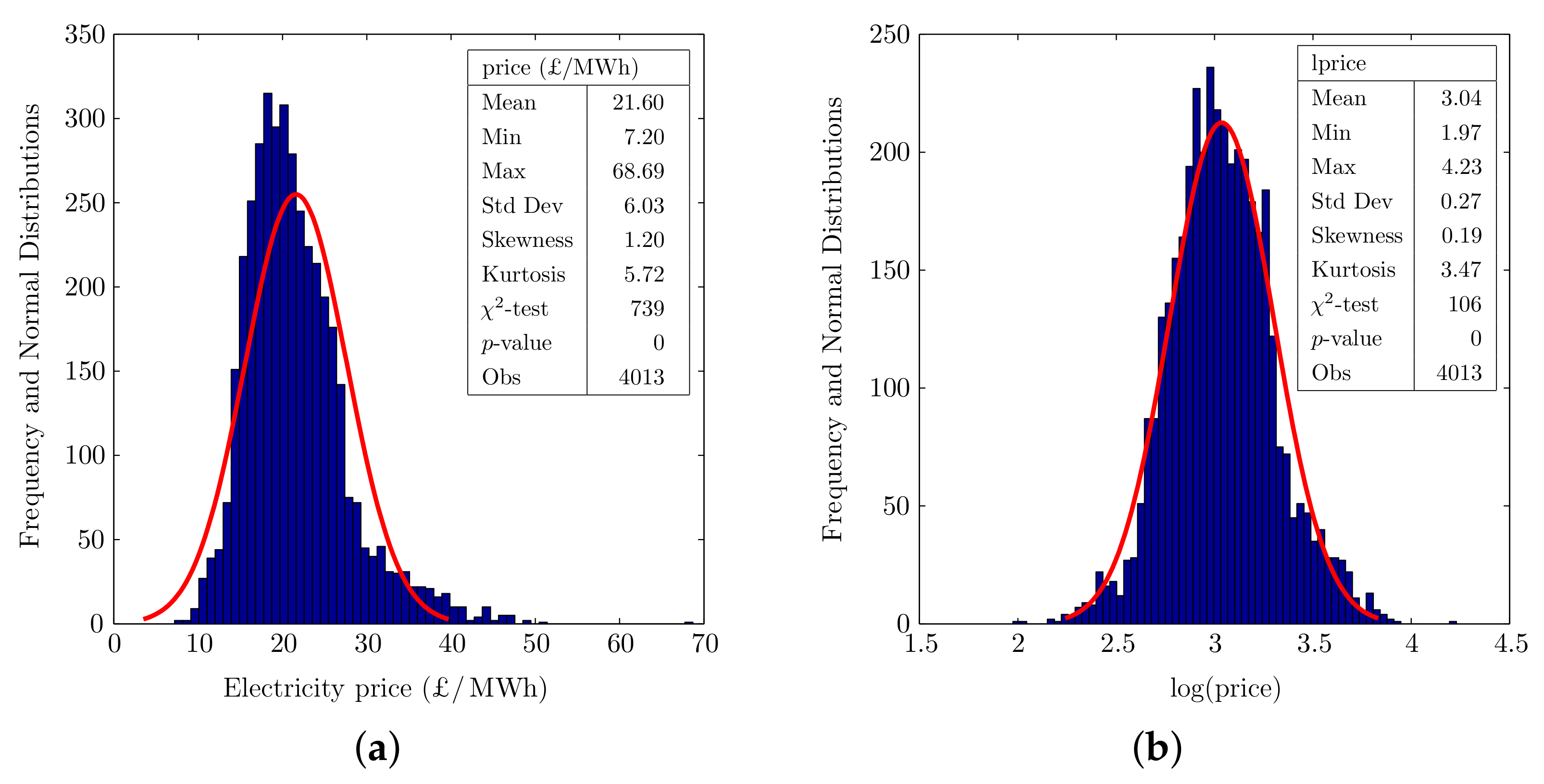
In Figure 1, we present the empirical distribution of demand weighted average prices (for short, we refer to as price). Pearson’s ${\chi }^2$ goodness of fit test concludes that prices and log prices (for short, we refer to as lprice) are not normally distributed. Indeed, the empirical distributions presented in Figure 1 are skewed to the right and have a peak higher than in the fitted normal distribution. The empirical distribution of lprice has also heavy tails reflecting rare observations scattered farther from the mean.

For these reasons we do not consider normal distribution as done, for example, in [6,7,8,9]. Our decision is consistent with [10], which highlights that there is ample evidence that data do not follow normal distribution. Replacing the assumption of normal distribution by a heavy-tailed distribution might improve forecast results [11].

Heavy tails are usually modeled by Student’s t distribution introduced in [12] or generalized error distribution (GED) introduced in [13]. According to [14], replacing normal or Student’s t distributions by GED is considered as more encouraging. GED is heavy tailed and has a higher peak compared to normal distribution. This distribution includes normal distribution as a special case. Moreover, GED does not have an issue of possible infinite unconditional moments as does Student’s t distribution. Some research (e.g., [15,16,17,18]) though consider normal or Student’s t distribution when applying the volatility model of [14] that was originally based on GED.

In order to model the feature of heavy tails, instead of normal distribution [19] assumes Student’s t distribution for model residuals. This approach however does not take into account asymmetry and the observation that GED may be more heavy tailed than Student’s t distribution.

Normal and Student’s t distributions have been recently used in volatility modeling in, for example, [20,21] even if the analyzed time series data are asymmetric. Earlier, [22] highlighted the importance of correctly modeling volatility of electricity prices in evaluating the deregulation experience, in forecasting, and in pricing electricity futures and other energy derivatives.

Other distributions applied in the literature are skew Student’s t distribution, skew generalized error distribution (SGED), and generalized hyperbolic distribution (GHD). In terms of accurately estimating the value at risk, [23] finds that a volatility model assuming skew Student’s t distribution outperforms volatility models based on normal and Student’s t distributions. In terms of forecast performance, however, [24] finds that skew Student’s t distribution does not outperform normal distribution. Forecasts of returns based on the SGED assumption are found to be more accurate than those when assuming normal and Student’s t distributions [25]. SGED is similarly used for modeling European call option prices in [26], the dynamics of electricity prices of the peak demand period over days in [5], and daily returns of carbon price time series in [27]. GHD and its special cases have been applied in various areas. For example, [28] applies GHD for modeling grain size distributions of wind blown sands, [29] applies for returns of daily prices of shares.

The paper is structured as follows. First we describe the volatility model. Then we verify in detail the two distributional assumptions (an i.i.d. and an assumed theoretical distribution) for model residuals of the estimated volatility model. Next the sign bias test is applied in order to verify the correctness of the estimated volatility model. Based on the correctly estimated volatility model we discuss the impact of reforms on price level and volatility. In the last section we draw our conclusions.

2. Methodology

2.1. Volatility Modeling

For modeling volatility of $lpric{e}_t$, representing the log of demand weighted average price of electricity during day t, we extend the original autoregressive and autoregressive conditional heteroscedasticity (AR–ARCH) volatility model introduced in [30] in the following way:

$$\mathrm{Mean\; equation:}lpric{e}_t=a_0+\sum _{i=1}^P{a}_{i}lpric{e}_{t-i}+w_t^{\prime }·b+{\epsilon }_t$$

(1)

$$\mathrm{Volatility\; equation:}{h}_t={\alpha }_0+\sum _{i=1}^p{\alpha }_i{\epsilon }_{t-i}^2+w_t^{\prime }·\delta$$

(2)

$$\mathrm{Two\; distributional\; assumptions:}{\nu }_t=\frac{{\epsilon }_t}{\sqrt{h_t}}i.i.d.\mathrm{SGED}(\mu =0,\sigma =1,\beta ,\chi )$$

(3)

The dependent variable $lpric{e}_t$ in the mean equation may depend on its past values through the AR process and exogenous variables. The AR process based on statistically significant lags of $lpric{e}_t$ allows taking into account partial adjustment effects and seasonality features. Exogenous variables included in vector $w_t$ are periodic functions and regime dummy variables corresponding to regulatory reforms. In modeling weekly seasonality, using periodic functions may be preferred to using daily dummy variables for obtaining a parsimonious model and for using dummy variables to denote regulatory regime periods. We do not consider fuel prices because they are available as quarterly average prices. Volatility $h_t$, modeled using the ARCH process in the second equation, can also depend on exogenous variables.

For the mean and volatility equations, we apply the maximum likelihood method, which requires assuming a distribution for model residuals. We assume that standardized residuals ${\nu }_t$ defined in the third equation are independent and identically distributed (i.i.d.) and follow SGED. The density of SGED is defined based on [31] proposing a general procedure for introducing skewness into a symmetric distribution in order to account for the presence of asymmetry. We also verify two alternative distributional assumptions of skew Student’s t introduced in [32] and GHD introduced in [28]. Details and statistical features of these distributions are described in the next section.

2.2. Statistical Features of SGED, Skew Student’s t Distributions, and GHD

SGED includes many other distributions as its special or limiting cases. These are GED, (skew) Laplace, (skew) normal, and uniform distributions.

SGED$(\mu ,\sigma ,\beta ,\chi )$ is characterized by four parameters: mean $\mu$, standard deviation $\sigma$, shape parameter $\beta$, and skewness parameter $\chi$. The shape parameter $\beta$ reflects the peak and tails of a distribution. The skewness parameter $\chi$ reflects asymmetry of a distribution. For example, when $\chi =1$, then the distribution is symmetric and we obtain GED$(\mu ,\sigma ,\beta )$ as a special case of SGED. Further, when $\beta =2$, then we obtain $\mathcal{N}(\mu ,\sigma )$.

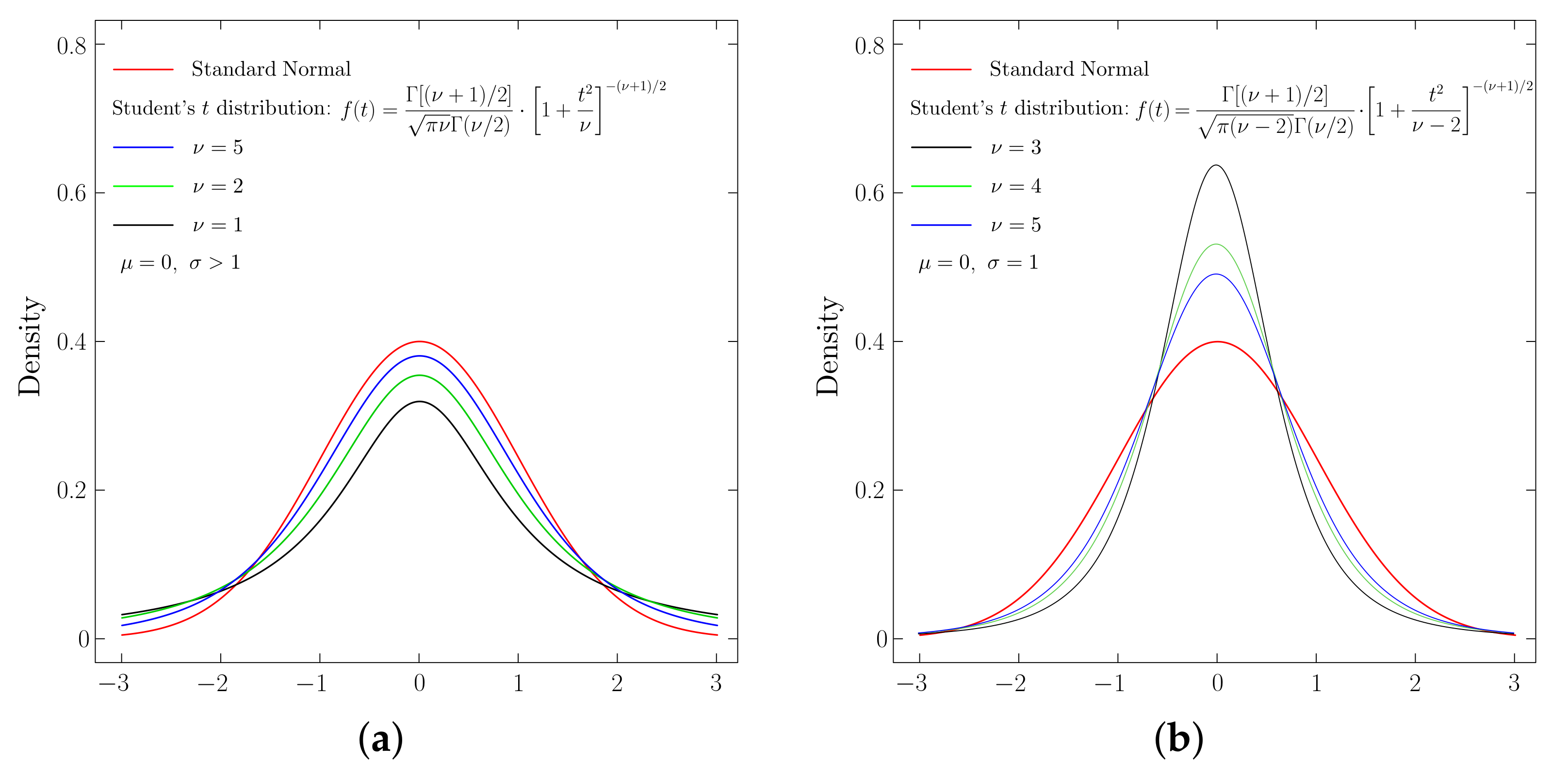
Student’s t distribution is another popularly used distribution for volatility modeling. Depending on the variance, there are two kinds of Student’s t distribution: with non-unit variance (described in Figure 2a) and with unit variance (described in Figure 2b).

Only in the non-unit variance case has Student’s t distribution noticeable heavy tails. Even if Student’s t distribution with non-unit variance has the desired feature of heavy tails, we cannot apply it because of two reasons. Firstly, its peak is lower than in normal distribution, which is opposite to what we observed in Figure 1. Secondly, the distributional assumption is needed for standardized residuals where we must have a unit variance as described in Equation (3). As described in Figure 2b, Student’s t distribution with unit variance does not have noticeable heavy tails. 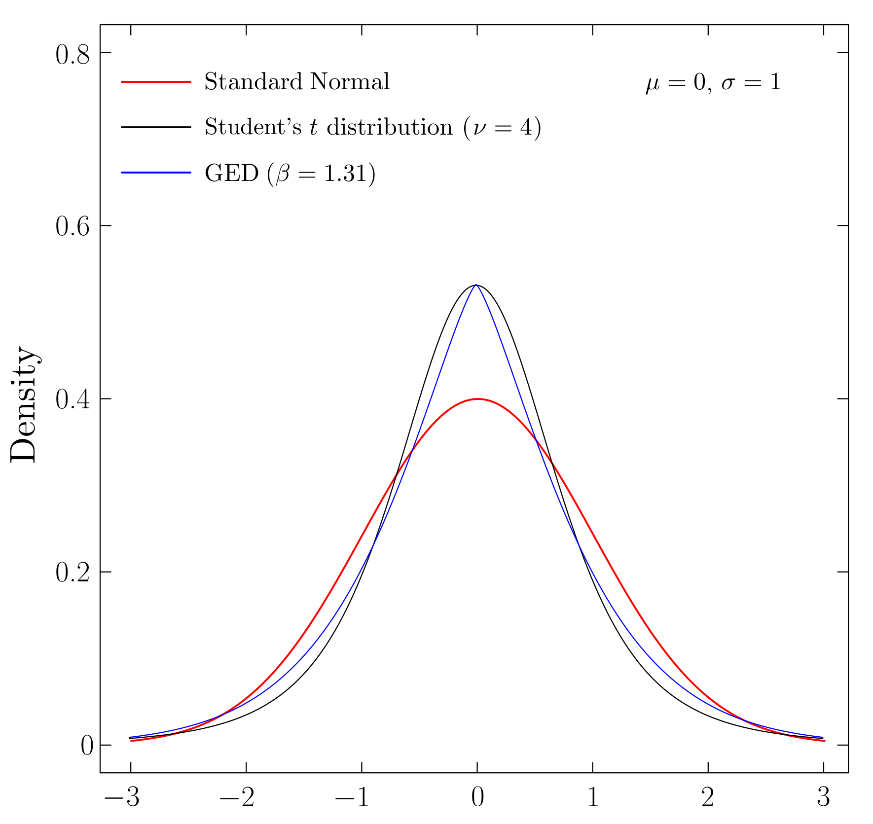Figure 3 presents a comparison of tails of Student’s t distribution of unit variance and GED. We observe that GED (a special case of SGED) can be more heavy tailed.

We consider skew Student’s t with unit variance as a possible alternative distribution to SGED. Skew Student’s t distribution depends on four parameters: mean $\mu$, standard deviation $\sigma$, the number of degrees of freedom $\nu$, and skewness parameter $\chi$. The number of degrees of freedom affects the peak and tails of the distribution as illustrated for its symmetric version (i.e., when $\chi =1$) in Figure 2b. Skew Student’s t distribution nests Student’s t, (skew) Cauchy, (skew) Gaussian or normal as its special or limiting cases.

We also consider GHD, which nests the following distributions as its special or limiting cases: hyperbolic, (variance, inverse) Gamma, (inverse, generalized inverse, normal inverse, skew) Gaussian, (skew) Student’s t, (skew) Cauchy, (skew) Laplace, and exponential.

3. Estimation Results

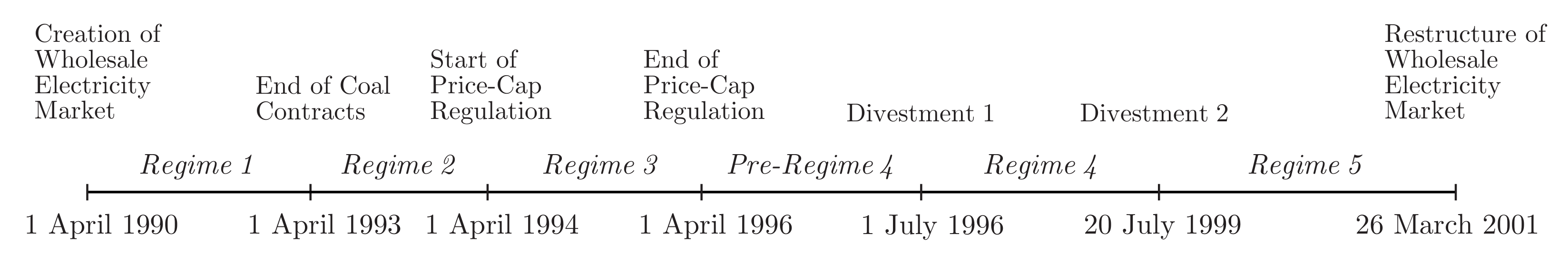
During the liberalization process, the regulatory authority introduced several reforms in the England and Wales electricity market. The regulatory reforms are described, for example, in [33,34]. In Figure 4, we summarize the timeline of those reforms.

Table 1. Summary statistics of demand weighted average electricity price over days during 1 April 1990–26 March 2001.

Price	Regime 1	Regime 2	Regime 3	Pre-Regime 4	Regime 4	Regime 5
	Apr. 90–Mar. 93	Apr. 93–Mar. 94	Apr. 94–Mar. 96	Apr. 96–Jul. 96	Jul. 96–Jul. 99	Jul. 99–Mar. 01
			Price-Cap Reg		Divestment 1	Divestment 2
Mean	20.21	24.59	20.89	20.64	23.42	19.97
Min	11.80	11.02	7.20	12.65	10.87	11.72
Max	32.21	31.12	68.69	34.94	50.45	34.26
St Dev	2.91	3.67	7.36	4.72	7.94	3.80
Coef of Var	14.42	14.94	35.21	22.86	33.92	19.04
Obs	1096	365	731	91	1114	616

contains summary statistics of demand weighted average price over days. The summary statistics show that during price-cap regulation, the average price level is lower but variance is higher. However, after the second series of divestments the price level and variance decreased. These findings are new and therefore motivate to analyze in more detail the price dynamics in relation to the regulatory reforms. The concepts of variance and volatility are not the same. The former corresponds to a sample variance and the latter corresponds to the definition of $h_t$ provided in the volatility equation.

In volatility modeling, we consider the log of demand weighted average price during day t (denoted as $lpric{e}_t$) because as presented in Figure 1b its empirical distribution is closer to normal distribution, which is a special case of SGED. A logarithmic transformation may also mitigate the effect of outliers observed in Figure 1a.

Prior to estimating the volatility model, we find that $lpric{e}_t$ is stationary, which allows applying the time and frequency domain analyses in order to determine the lag structure and periodic functions with required frequencies. These are needed for modeling the partial adjustment effects and seasonality pattern (i.e., daily, weekly, annual seasonalities) of electricity prices.

Based on the methodology described in the previous section, we present estimation results of the volatility model in

Table 2. Estimation results when assuming SGED.

Mean Equation					Volatility Equation
${\displaystyle {\mathit{lprice}}_{\mathit{t}}={\mathit{a}}_{\mathbf{0}}+\sum _{\mathit{i}=\mathbf{1}}^{\mathit{P}}{\mathit{a}}_{\mathit{i}}{\mathit{lprice}}_{\mathit{t}-\mathit{i}}+{\mathit{w}}_{\mathit{t}}^{\prime }·\mathit{b}+{\mathit{\epsilon }}_{\mathit{t}}}$					${\displaystyle {\mathit{h}}_{\mathit{t}}={\mathit{\alpha }}_{\mathbf{0}}+\sum _{\mathit{i}=\mathbf{1}}^{\mathbf{p}}{\mathit{\alpha }}_{\mathit{i}}{\mathit{\epsilon }}_{\mathit{t}-\mathit{i}}^{\mathbf{2}}+{\mathit{w}}_{\mathit{t}}^{\prime }·\mathit{\delta }}$
Variable	Coef		Std Err		Variable	Coef		Std Err
$a_0$	0.0566	***	0.0037		${\alpha }_0$	0.0012	***	0.0001
$lpric{e}_{t-1}$	0.5763	***	0.0006		${\epsilon }_{t-1}^2$	0.2041	***	0.0286
$lpric{e}_{t-2}$	0.0799	***	0.0020		${\epsilon }_{t-3}^2$	0.0176		0.0114
$lpric{e}_{t-3}$	0.0579	***	0.0013		${\epsilon }_{t-4}^2$	0.0402	**	0.0158
$lpric{e}_{t-4}$	0.0448	***	0.0014		${\epsilon }_{t-5}^2$	0.0814	***	0.0217
$lpric{e}_{t-6}$	0.0658	***	0.0015		${\epsilon }_{t-6}^2$	0.0284	*	0.0157
$lpric{e}_{t-7}$	0.2302	***	0.0011		${\epsilon }_{t-7}^2$	0.1670	***	0.0284
$lpric{e}_{t-8}$	−0.0735	***	0.0019		$cos(6\pi t/7)$	0.0006	***	0.0001
$lpric{e}_{t-9}$	−0.1125	***	0.0017		$sin(2\pi t/7)$	0.0006	***	0.0001
$lpric{e}_{t-14}$	0.0617	***	0.0015		$sin(6\pi t/7)$	−0.0008	***	0.0001
$lpric{e}_{t-21}$	0.1213	***	0.0016		Regime 2	0.0001		0.0002
$lpric{e}_{t-22}$	−0.0930	***	0.0026		Regime 3	0.0060	***	0.0009
$lpric{e}_{t-25}$	−0.0415	***	0.0018		Pre-Regime 4	0.0109	***	0.0042
$lpric{e}_{t-28}$	0.0861	***	0.0024		Regime 4	0.0079	***	0.0009
$lpric{e}_{t-29}$	−0.0602	***	0.0014		Regime 5	0.0047	***	0.0007
$lpric{e}_{t-35}$	0.0667	***	0.0017
$lpric{e}_{t-36}$	−0.0750	***	0.0019		SGED parameters
$lpric{e}_{t-42}$	0.0335	***	0.0041		$\widehat{\beta }$	1.2802	***	0.0384
$lpric{e}_{t-49}$	0.0574	***	0.0012		$\widehat{\chi }$	1.0458	***	0.0179
$lpric{e}_{t-50}$	−0.0812	***	0.0020
$lpric{e}_{t-56}$	0.0560	***	0.0012
$lpric{e}_{t-61}$	−0.0444	***	0.0014
$lpric{e}_{t-63}$	0.0365	***	0.0032
$lpric{e}_{t-71}$	−0.0433	***	0.0015
$lpric{e}_{t-108}$	−0.0209	***	0.0014
$lpric{e}_{t-147}$	0.0228	***	0.0014
$lpric{e}_{t-225}$	−0.0167	***	0.0013
$lpric{e}_{t-364}$	0.0489	***	0.0013
$cos(2\pi t/7)$	−0.0041	***	0.0015
$sin(6\pi t/7)$	−0.0060	***	0.0004
Regime 2	0.0010		0.0018
Regime 3	−0.0166	***	0.0042
Pre-Regime 4	−0.0038		0.0165
Regime 4	−0.0033		0.0032
Regime 5	−0.0131	***	0.0041

Notes: Even if the p-value ≈ 0.12 of ${\mathit{\epsilon }}_{\mathit{t}-\mathit{3}}^{\mathit{2}}$ is slightly above 10% in the estimated model, we keep this term in order to satisfy the i.i.d. assumption. *, **, and *** stand for the 10%, 5%, and 1% significance levels, respectively.

.

In volatility modeling we assumed that standardized residuals ${\displaystyle {\nu }_t=\frac{{\epsilon }_t}{\sqrt{h_t}}}$ are i.i.d. and follow SGED$(\mu =0,\sigma =1,\beta ,\chi )$. Using the Q-test proposed in [39] and BDS-test further developed in [40], we find that the standardized residuals and standardized residuals squared of the estimated volatility model are not serially correlated and are i.i.d. The results are presented in

Table A1. Q-test for standardized residuals when assuming SGED.

Lag		Q-Test	p-Value		Q-Test	p-Value
1		0.05	0.82		0.22	0.64
10		11.80	0.30		7.60	0.67
20		25.99	0.17		20.49	0.43
30		35.36	0.23		29.61	0.49
100		97.43	0.55		94.37	0.64
200		188.60	0.71		182.25	0.81
300		275.47	0.84		283.21	0.75
		$H_0:{\nu }_t$ has no serial correlation			$H_0:{\nu }_t^2$ has no serial correlation

Note: No serial correlation in ${\nu }_t$ is interpreted as νt being homoscedastic.

and

Table A2. BDS-test for standardized residuals when assuming SGED.

Dimension	BDS-Test	p-Value		BDS-Test	p-Value
2	−0.0004	0.77		−0.0022	0.33
3	0.0024	0.26		0.0018	0.61
4	0.0030	0.22		0.0032	0.45
5	0.0034	0.19		0.0034	0.44
6	0.0034	0.17		0.0032	0.46
	$H_0:{\nu }_t$ is i.i.d.			$H_0:{\nu }_t^2$ is i.i.d.

, respectively.

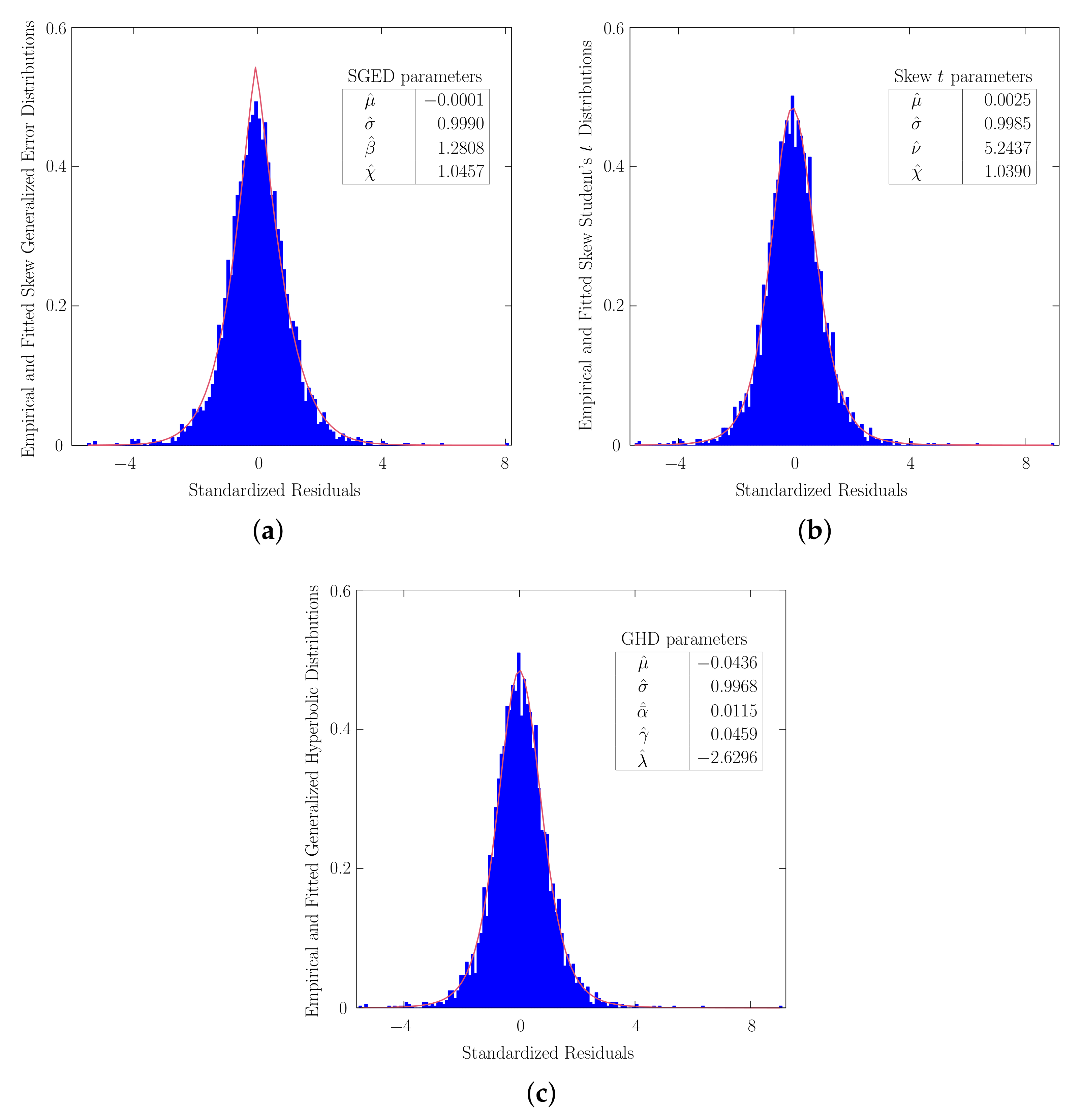
We estimated the volatility model under three distributional assumptions: SGED$(\mu =0,\sigma =1,\beta ,\chi )$, skew Student’s t$(\mu =0,\sigma =1,\nu ,\chi )$, and GHD$(\mu =0,\sigma =1,\overline{\alpha },\gamma ,\lambda )$. In Figure 5a–c we present the empirical distributions of standardized residuals superimposed by the fitted SGED, skew Student’s t, and GHD, respectively. Visually, all theoretical distributions provide a good match for the empirical distributions. This is also confirmed statistically by the goodness of fit test.

The distributional parameters of SGED estimated through the volatility model presented in Table 2 and estimated through fitting of standardized residuals ${\widehat{\nu }}_t$ presented in Figure 5a are about the same. Both approaches are based on the maximum likelihood estimation.

For the first estimated volatility model based on SGED we perform additional tests for the shape parameter $\beta$ and skewness parameter $\chi$. When $\beta =2$ and $\chi =1$, then SGED narrows down to normal distribution. We reject $H_0:\beta =2$, which suggests that the empirical distribution of standardized residuals has a higher peak and heavy tails compared to normal distribution (because $\widehat{\beta }\approx 1.28<2$). Further rejecting $H_0:\chi =1$ suggests that the empirical distribution is also asymmetric (more precisely skewed to the right because $\widehat{\chi }\approx 1.05>1$).

Similarly, for the second estimated volatility model based on skew Student’s t distribution we test asymmetry of the empirical distribution of standardized residuals. As presented in

Table A4. Estimation results when assuming skew Student’s t distribution.

Mean Equation					Volatility Equation
${\displaystyle {\mathit{lprice}}_{\mathit{t}}={\mathit{a}}_{\mathbf{0}}+\sum _{\mathit{i}=\mathbf{1}}^{\mathit{P}}{\mathit{a}}_{\mathit{i}}{\mathit{lprice}}_{\mathit{t}-\mathit{i}}+{\mathit{w}}_{\mathit{t}}^{\prime }·\mathit{b}+{\mathit{\epsilon }}_{\mathit{t}}}$					${\displaystyle {\mathit{h}}_{\mathit{t}}={\mathit{\alpha }}_{\mathbf{0}}+\sum _{\mathit{i}=\mathbf{1}}^{\mathbf{p}}{\mathit{\alpha }}_{\mathit{i}}{\mathit{\epsilon }}_{\mathit{t}-\mathit{i}}^{\mathbf{2}}+{\mathit{w}}_{\mathit{t}}^{\prime }·\mathit{\delta }}$
Variable	Coef		Std Err		Variable	Coef		Std Err
$a_0$	0.0467		0.0329		${\alpha }_0$	0.0012	***	0.0001
$lpric{e}_{t-1}$	0.5794	***	0.0001		${\epsilon }_{t-1}^2$	0.2209	***	0.0300
$lpric{e}_{t-2}$	0.0741	***	0.0059		${\epsilon }_{t-3}^2$	0.0132		0.0118
$lpric{e}_{t-3}$	0.0596	***	0.0065		${\epsilon }_{t-4}^2$	0.0474	***	0.0169
$lpric{e}_{t-4}$	0.0459	***	0.0066		${\epsilon }_{t-5}^2$	0.0719	***	0.0220
$lpric{e}_{t-6}$	0.0650	***	0.0061		${\epsilon }_{t-6}^2$	0.0223		0.0164
$lpric{e}_{t-7}$	0.2380	***	0.0011		${\epsilon }_{t-7}^2$	0.1769	***	0.0300
$lpric{e}_{t-8}$	−0.0829	***	0.0058		$cos(6\pi t/7)$	0.0008	***	0.0001
$lpric{e}_{t-9}$	−0.1115	***	0.0047		$sin(2\pi t/7)$	0.0006	***	0.0001
$lpric{e}_{t-14}$	0.0695	***	0.0061		$sin(6\pi t/7)$	−0.0008	***	0.0002
$lpric{e}_{t-21}$	0.1151	***	0.0045		Regime 2	0.0000		0.0002
$lpric{e}_{t-22}$	−0.0872	***	0.0056		Regime 3	0.0059	***	0.0009
$lpric{e}_{t-25}$	−0.0395	***	0.0064		Pre-Regime 4	0.0120	***	0.0044
$lpric{e}_{t-28}$	0.0849	***	0.0056		Regime 4	0.0081	***	0.0010
$lpric{e}_{t-29}$	−0.0619	***	0.0065		Regime 5	0.0051	***	0.0007
$lpric{e}_{t-35}$	0.0624	***	0.0067
$lpric{e}_{t-36}$	−0.0753	***	0.0059		Skew Student’s t parameters
$lpric{e}_{t-42}$	0.0385	***	0.0069		$\widehat{\nu }$	5.2192	***	0.4413
$lpric{e}_{t-49}$	0.0590	***	0.0068		$\widehat{\chi }$	1.0376	***	0.0247
$lpric{e}_{t-50}$	−0.0844	***	0.0055
$lpric{e}_{t-56}$	0.0528	***	0.0068
$lpric{e}_{t-61}$	−0.0431	***	0.0059
$lpric{e}_{t-63}$	0.0341	***	0.0071
$lpric{e}_{t-71}$	−0.0386	***	0.0062
$lpric{e}_{t-108}$	−0.0210	***	0.0062
$lpric{e}_{t-147}$	0.0206	***	0.0061
$lpric{e}_{t-225}$	−0.0170	***	0.0057
$lpric{e}_{t-364}$	0.0500	***	0.0055
$cos(2\pi t/7)$	−0.0039	**	0.0018
$sin(6\pi t/7)$	−0.0065	***	0.0014
Regime 2	0.0006		0.0030
Regime 3	−0.0141	***	0.0043
Pre-Regime 4	−0.0087		0.0149
Regime 4	−0.0021		0.0037
Regime 5	−0.0127	***	0.0041

Notes: The p-values of ${\mathit{\epsilon }}_{\mathit{t}-\mathit{3}}^{\mathit{2}}$ and ${\mathit{\epsilon }}_{\mathit{t}-\mathit{6}}^{\mathit{2}}$ are approximately 0.26 and 0.18, respectively. We keep these terms in order to satisfy the i.i.d. assumption. ** and *** stand for the 5% and 1% significance levels, respectively.

, we obtain $\widehat{\chi }\approx 1.038$ with its standard error of approximately $0.0247$. Using these results we do not reject $H_0:\chi =1$, which implies that the empirical distribution of standardized residuals is symmetric.

The asymmetry of standardized residuals under all distributional assumptions can also be tested based on the skewness coefficient following [41]. The test results of skewness coefficient presented in

Table 3. Testing symmetry of empirical distribution of standardized residuals ${\widehat{\nu }}_t$ using the skewness coefficient.

	Sample Skewness (${\mathit{G}}_1$)	Std Err of ${\mathit{G}}_1$	Test Value	Decision for ${\mathit{H}}_0:\mathbf{Skewness}=0$
${\widehat{\nu }}_t$ based on SGED	0.1682	0.0405	4.15	Reject
${\widehat{\nu }}_t$ based on Skew t	0.2041	0.0405	5.03	Reject
${\widehat{\nu }}_t$ based on GHD	0.2059	0.0405	5.08	Reject

suggest that the empirical distributions of standardized residuals ${\widehat{\nu }}_t$ are asymmetric in all volatility models. In the first volatility model we assumed standardized residuals ${\nu }_t$ following SGED, in the second—skew Student’s t distribution, and in the third—GHD. The conclusion of asymmetry of the empirical distribution of standardized residuals from the second volatility model is however in contradiction with the earlier test of skewness parameter from skew Student’s t distribution, which suggested that the empirical distribution of standardized residuals is symmetric.

Another contradiction is related to the significance of the ARCH terms. We obtain two statistically insignificant ARCH terms when assuming skew Student’s t distribution and GHD (Table A4 and

Table A5. Estimation results when assuming GHD.

Mean Equation					Volatility Equation
${\displaystyle {\mathit{lprice}}_{\mathit{t}}={\mathit{a}}_{\mathbf{0}}+\sum _{\mathit{i}=\mathbf{1}}^{\mathit{P}}{\mathit{a}}_{\mathit{i}}{\mathit{lprice}}_{\mathit{t}-\mathit{i}}+{\mathit{w}}_{\mathit{t}}^{\prime }·\mathit{b}+{\mathit{\epsilon }}_{\mathit{t}}}$					${\displaystyle {\mathit{h}}_{\mathit{t}}={\mathit{\alpha }}_{\mathbf{0}}+\sum _{\mathit{i}=\mathbf{1}}^{\mathbf{p}}{\mathit{\alpha }}_{\mathit{i}}{\mathit{\epsilon }}_{\mathit{t}-\mathit{i}}^{\mathbf{2}}+{\mathit{w}}_{\mathit{t}}^{\prime }·\mathit{\delta }}$
Variable	Coef		Std Err		Variable	Coef		Std Err
$a_0$	0.0452		0.0381		${\alpha }_0$	0.0012	***	0.0001
$lpric{e}_{t-1}$	0.5798	***	0.0004		${\epsilon }_{t-1}^2$	0.2200	***	0.0302
$lpric{e}_{t-2}$	0.0741	***	0.0106		${\epsilon }_{t-3}^2$	0.0134		0.0119
$lpric{e}_{t-3}$	0.0598	***	0.0123		${\epsilon }_{t-4}^2$	0.0476	***	0.0169
$lpric{e}_{t-4}$	0.0457	***	0.0116		${\epsilon }_{t-5}^2$	0.0718	***	0.0221
$lpric{e}_{t-6}$	0.0648	***	0.0101		${\epsilon }_{t-6}^2$	0.0223		0.0164
$lpric{e}_{t-7}$	0.2389	***	0.0016		${\epsilon }_{t-7}^2$	0.1779	***	0.0304
$lpric{e}_{t-8}$	−0.0838	***	0.0096		$cos(6\pi t/7)$	0.0008	***	0.0001
$lpric{e}_{t-9}$	−0.1119	***	0.0060		$sin(2\pi t/7)$	0.0007	***	0.0001
$lpric{e}_{t-14}$	0.0702	***	0.0102		$sin(6\pi t/7)$	−0.0008	***	0.0002
$lpric{e}_{t-21}$	0.1138	***	0.0058		Regime 2		0.0000	0.0002
$lpric{e}_{t-22}$	−0.0864	***	0.0089		Regime 3	0.0059	***	0.0009
$lpric{e}_{t-25}$	−0.0393	***	0.0098		Pre-Regime 4	0.0120	***	0.0044
$lpric{e}_{t-28}$	0.0847	***	0.0094		Regime 4	0.0081	***	0.0010
$lpric{e}_{t-29}$	−0.0616	***	0.0111		Regime 5	0.0051	***	0.0007
$lpric{e}_{t-35}$	0.0625	***	0.0125
$lpric{e}_{t-36}$	−0.0757	***	0.0103		GHD parameters
$lpric{e}_{t-42}$	0.0390	***	0.0106		shape	0.0252		0.0231
$lpric{e}_{t-49}$	0.0591	***	0.0124		skewness	0.9527	***	0.0151
$lpric{e}_{t-50}$	−0.0847	***	0.0090		$\widehat{\lambda }$	−2.6159	***	0.2224
$lpric{e}_{t-56}$	0.0530	***	0.0112
$lpric{e}_{t-61}$	−0.0427	***	0.0081
$lpric{e}_{t-63}$	0.0337	***	0.0108
$lpric{e}_{t-71}$	−0.0389	***	0.0087
$lpric{e}_{t-108}$	−0.0206	***	0.0068
$lpric{e}_{t-147}$	0.0207	***	0.0065
$lpric{e}_{t-225}$	−0.0171	***	0.0059
$lpric{e}_{t-364}$	0.0498	***	0.0069
$cos(2\pi t/7)$	−0.0040	**	0.0020
$sin(6\pi t/7)$	−0.0065	***	0.0015
Regime 2	0.0004		0.0033
Regime 3	−0.0143	***	0.0044
Pre-Regime 4	−0.0083		0.0149
Regime 4	−0.0023		0.0038
Regime 5	−0.0128	***	0.0042

Notes: The p-values of ${\mathit{\epsilon }}_{\mathit{t}-\mathit{3}}^{\mathit{2}}$ and ${\mathit{\epsilon }}_{\mathit{t}-\mathit{6}}^{\mathit{2}}$ are approximately 0.26 and 0.18, respectively. We keep these terms in order to satisfy the i.i.d. assumption. ** and *** stand for the 5% and 1% significance levels, respectively.

). Excluding the statistically insignificant ARCH terms led to violation of the i.i.d. assumption.

The appropriateness of the distributional assumption (SGED, skew Student’s t distribution, or GHD) for standardized residuals can be verified using the Kullback–Leibler distance, which is a general methodology for comparing the distance between the empirical and theoretical distributions [42]. For most values of k presented in

Table 4. Kullback–Leibler distance for the empirical distributions of standardized residuals when comparing to SGED, skew Student’s t distribution, and GHD.

	Assumed Distributions
k	SGED	Skew Student’s t	GHD
1	0.0244	0.0438	0.0293
2	0.0359	0.0242	0.0365
3	0.0090	0.0173	0.0542
4	0.0060	0.0182	0.0367
5	0.0098	0.0421	0.0164
6	0.0012	0.0369	0.0182
7	0.0001	0.0308	0.0196
8	0.0035	0.0255	0.0114
9	0.0013	0.0138	0.0158
10	0.0054	0.0186	0.0153
11	0.0114	0.0195	0.0167
12	0.0068	0.0277	0.0147
13	0.0024	0.0218	0.0113
14	0.0006	0.0158	0.0099
15	0.0050	0.0185	0.0046
16	0.0084	0.0137	0.0044
17	0.0077	0.0135	0.0001
18	0.0055	0.0092	0.0007
19	0.0031	0.0118	0.0028
20	0.0013	0.0087	0.0036

Notes: The Kullback–Leibler distance allows to determine how close an empirical distribution is to a theoretical probability distribution [42]. k is the number of values in the nearest neighbor search algorithm. The default number of values is usually set to 10.

, the Kullback–Leibler distance is smaller when comparing the empirical distribution of standardized residuals from the first volatility model to SGED.

Therefore, taking into account the contradiction of asymmetry test results when assuming skew Student’s t, statistically insignificant ARCH terms and a greater Kullback–Leibler distance when assuming skew Student’s t or GHD, we suggest that in our research SGED provides a better distributional fit for model residuals than do skew Student’s t distribution or GHD.

Even if both distributional assumptions for standardized residuals are satisfied (an i.i.d. and SGED), the estimated volatility model may still be incorrect because of possible remaining asymmetries in the effect of positive and negative shocks on volatility. That is why, in order to evaluate the correctness of the volatility model we perform the sign bias test, where the null hypothesis states that the volatility model is correctly specified. Based on the test results in

Table A3. t-test values of the sign bias test for standardized residuals when assuming SGED.

	t-Test	p-Value
Sign Bias	0.32	0.75
Negative Sign Bias	0.39	0.69
Positive Sign Bias	0.88	0.38
Joint Effect	2.44	0.49

, we do not reject the null hypothesis. This suggests that the volatility model is correctly specified.

The estimated volatility model explains about 80% of variation in the price data and partially confirms the preliminary results from Table 1. In the next section, after discussing our methodological contributions, we discuss in detail the impact of regulatory reforms on price level and volatility.

4. Discussion

Among others, there are two distributions popularly applied in modeling the dynamics of energy price data: normal and Student’s t. Sometimes the reason for preferring Student’s t distribution to normal distribution was to model the presence of heavy tails reflecting a higher probability of occurrence of extreme values than under normal distribution [19]. In Figure 3 we showed that under the same peak, GED (a special case of SGED) can be more heavy tailed. Another possible alternative distribution considered in this paper is GHD, which also nests many distributions as its special or limiting cases.

If the distributional assumption is not satisfied, then a quasi maximum likelihood estimation introduced in [43] could be used. This methodology addresses the model misspecification problem related to the wrong theoretical distributional assumption and allows statistical inferences to be drawn robustly. For example, ref. [44] models the dynamics of electricity prices from various countries assuming a normal distribution, even if prices are asymmetric and have platykurtic and leptokurtic distributions. For statistical inference the research applies robust standard errors following [43]. However, due to the wrong assumption of normal distribution, we believe that the results in [44] based on the maximum likelihood estimation may be biased.

Only few papers discuss the empirical distribution of model residuals in order to check if the distributional assumptions (an i.i.d. and an assumed theoretical distribution) were satisfied or not. After verifying the two distributional assumptions, it was necessary to check if the estimated volatility model is correct using the sign bias test. Given that the distributional assumptions and estimated volatility model are correct, it is possible to proceed to the interpretation of our results, that is, the impact of regulatory reforms on price level and volatility.

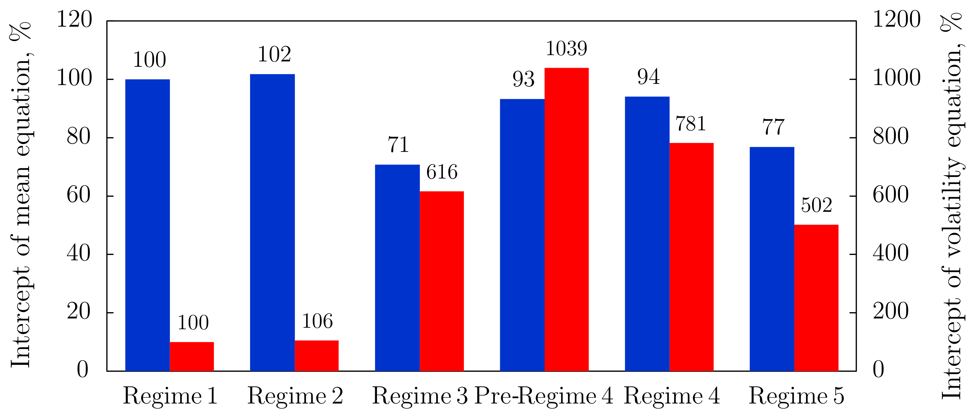
In

Table 5. Analysis of the impact of regulatory reforms.

Price Level					Price Volatility
Variable	Coef		Std Err		Variable	Coef		Std Err
$a_0$	0.0566	***	0.0037		${\alpha }_0$	0.0012	***	0.0001
Regime 2	0.0010		0.0018		Regime 2	0.0001		0.0002
Regime 3	−0.0166	***	0.0042		Regime 3	0.0060	***	0.0009
Pre-Regime 4	−0.0038		0.0165		Pre-Regime 4	0.0109	***	0.0042
Regime 4	−0.0033		0.0032		Regime 4	0.0079	***	0.0009
Regime 5	−0.0131	***	0.0041		Regime 5	0.0047	***	0.0007

Note: *** stand for the 1% significance level.

we provide an excerpt from Table 2, which contains coefficient estimates in front of regime dummy variables. These coefficient estimates from the mean and volatility equations indicate changes in the price level and volatility, respectively, compared to Regime 1, i.e., the reference period during 1 April 1990 to 31 March 1993.

For the qualitative analysis we recalculate intercept terms of the mean and volatility equations in percentages, where the intercept term for the reference period, i.e., Regime 1, is set equal to 100%. The calculations are summarized in Figure 6.

The estimate of coefficient in front of Regime 2 (after coal contracts expired on 31 March 1993 and before price-cap regulation started on 1 April 1994) in the volatility equation is almost zero. This suggests that price volatility was about the same during Regime 1 (i.e., 1 April 1990 to 31 March 1993) and Regime 2 (i.e., 1 April 1993 to 31 March 1994). Our result does not necessarily contradict to the finding in [2], which documents increased price volatility after the expiry of coal contracts because the research considered arithmetic average price over weeks.

We find that compared to the reference period, during price-cap regulation, that is, Regime 3 (i.e., 1 April 1994 to 31 March 1996) the price level is lower (i.e., $0.0566+(-0.0166)=0.04$ or 71% for Regime 3 is lower than $0.0566$ or 100% for Regime 1), which however takes place at the cost of increased price volatility (i.e., $0.0012+0.0060=0.0072$ or 616% for Regime 3 is higher than $0.0012$ or 100% for Regime 1). Generally, higher price volatility may be stemming from different bidding strategies discussed in [4,45]. After the first series of divestments (i.e., Regime 4) price level and volatility are higher than during price-cap regulation (i.e., Regime 3).

From the estimated volatility model, it is not possible to state that the second series of divestments (i.e., Regime 5) was more successful than price-cap regulation (i.e., Regime 3). This is because compared to price-cap regulation, after the second series of divestments price level is higher (i.e., $0.0566+(-0.0131)=0.0435$ or 77% for Regime 5 is greater than $0.0566+(-0.0166)=0.04$ or 71% for Regime 3) and price volatility is lower ($0.0012+0.0047=0.0059$ or 502% for Regime 5 is less than $0.0012+0.0060=0.0072$ or 1039% for Regime 3). But had we used only the results of summary statistics of demand weighted average prices of electricity presented in Table 1, we would have stated that the second series of divestments was more successful than price-cap regulation because average level and variance of prices were lower after the second series of divestments was introduced.

We find that the second series of divestments was more successful than the first series at decreasing the price level (i.e., $0.0566+(-0.0131)=0.0435$ or 77% for Regime 5 is lower than $0.0566+(-0.0033)=0.0533$ or 94% for Regime 4) and price volatility (i.e., $0.0012+0.0047=0.0059$ or 502% for Regime 5 is lower than $0.0012+0.0079=0.0091$ or 781% for Regime 4). The changes observed after the second series of divestments are statistically significant.

5. Conclusions

Modeling volatility of energy prices is of interest to investors, producers, and market regulators. Various models have been applied in analyzing price volatility, most of which however have assumed normal or Student’s t distributions. The empirical distribution of data or model residuals usually does not follow normal or Student’s t distributions due to asymmetry, excess kurtosis, a higher peak than in normal distribution or heavy tails. That is why we conclude that in such cases, the assumption of normal or Student’s t distributions should be replaced by SGED. Alternatively, in some cases skew Student’s t distribution with unit variance or GHD could be also considered.

Because testing asymmetry under the assumption of skew Student’s t distribution led to contradictory conclusions, some ARCH terms were found statistically insignificant and the value of the Kullback–Leibler distance was mostly greater when assuming skew Student’s t distribution or GHD, we conclude that SGED is more appropriate for modeling the volatility of our price data. According to [46], correct modelling of price volatility is important for building accurate pricing models, for forecasting future price volatility, and for enriching our understanding of the broader financial markets, the energy industry, and the overall economy.

SGED could be used in more complex volatility models, too. In some cases complicating a volatility model may become unnecessary if one assumes a flexible distribution capturing such features as asymmetry, heavy tails, or a higher peak than in normal distribution. Correctly estimated volatility models can reliably be used for policy analysis or forecast.

Our volatility model includes a vector of explanatory variables. This vector can be generalized to include market shares of firms, renewable energy sources, fuel prices, or other variables, when analyzing current energy markets. In most cases, this adaptation however would depend on the availability and completeness of data.

Interestingly, we find that conclusions based on summary statistics and estimated volatility model are not qualitatively the same. Based on summary statistics one would conclude that the second series of divestments was more successful than price-cap regulation because both price level and variance are lower. However, based on the estimated volatility model, we find that compared to price-cap regulation, the price level is higher after the second series of divestments, although the difference between coefficient estimates is not large (0.0435 versus 0.04). We also find that the second series of divestments was more successful than the first series at reducing the price level and volatility. Therefore, we conclude that divestment series might be preferred because they may allow reducing the influence of big companies, improving competition, and avoiding monitoring costs arising under price-cap regulation.

Demand weighted average prices have not been analyzed much in the literature probably due to limitations of data on demand. We believe that distinguishing between arithmetic and weighted averages is important because the former assumes the same weight regardless of demand or traded volumes in various trading periods over days. Our results and conclusions could be of interest to regulators and investors in markets, which were formed based on the original model of the England and Wales electricity market.