Article

Analyzing Medical Data by Using Statistical Learning Models

1
Department of Mathematical Sciences and Computational Science Program, University of Texas at El Paso, El Paso, TX 79968, USA
2
Computational Science Program, University of Texas at El Paso, El Paso, TX 79968, USA
3
Department of Data Science, Ramapo College of New Jersey, Mahwah, NJ 07430, USA
*
Author to whom correspondence should be addressed.
Mathematics 2021, 9(9), 968; https://doi.org/10.3390/math9090968
Submission received: 3 February 2021 / Revised: 21 April 2021 / Accepted: 22 April 2021 / Published: 26 April 2021

Abstract

:
In this work, we investigated the prognosis of three medical data specifically, breast cancer, heart disease, and prostate cancer by using 10 machine learning models. We applied all 10 models to each dataset to identify patterns in them. Furthermore, we use the models to diagnose risk factors that increases the chance of these diseases. All the statistical learning techniques discussed were grouped into linear and nonlinear models based on their similarities and learning styles. The models performances were significantly improved by selecting models while taking into account the bias-variance tradeoffs and using cross-validation for selecting the tuning parameter. Our results suggests that no particular class of models or learning style dominated the prognosis and diagnosis for all three medical datasets. However nonlinear models gave the best predictive performance for breast cancer data. Linear models on the other hand gave the best predictive performance for heart disease data and a combination of linear and nonlinear models for the prostate cancer dataset.

1. Introduction

Statistical learning models have been applied in detection and classification of many chronic diseases including cancer, heart disease, tumor, diabetes, and several others (see [1,2,3,4]). These methods aid practitioners and researchers to understand beyond given observations to detect trends and patterns in unseen datasets. In addition, some of these models help to identify factors that play a role in the cause of these diseases. In addition to the medical field, statistical learning models have been applied to problems in several industrial and scientific fields such as malware detection [5] and spacecraft autonomy modeling [6].
Annually, more than 350,000 death are recorded for prostate cancer, making it the second most common cancer among males [7]. Since about one million new cases are reported yearly, accurate diagnostics is the key to reduce mortality. Diagnosis of prostate cancer is based on the prostate tissue biopsies grading where tissue samples are examined and scored by a pathologist [7]. Using Bivariate and multivariate analyses, Stamey [4] showed cancer volume to be the primary determinant of serum prostate specific antigen levels. Hastie [8] applied different predictive models including PCR, PLS, lasso, ridge, and the best subset regression to assess risk factors of prostate cancer. They concluded that volume of prostate cancer is a significant predictor of prostate cancer.
The mortality rate of breast cancer (BC) has been increasing in the past decades [9]. In the United States, the probability that a randomly selected woman will have breast cancer in her life time is about 12 % . However, the death rate has declined over the past years with the use of statistical learning methods. Recent analysis shows that the rate of survival is 91 % after 5 years of diagnosis and 80 % after 15 years [9]. Chaurasia [10] compares different classification models such as support vector machine with radial basis function (SVM-RBF) kernel, naive Bayes, decision trees, and radial basis function neural networks to determine the optimal model for breast cancer data. They concluded SVM-RBF kernel to be the most accurate ( 96.84 % ) classifier. Joachims [11] used neuron-fuzzy model to achieve prediction accuracy of 95.06 % . Several methods have been used by other researchers including SVM, k-nearest neighbor algorithm (IBK), and Bloom Filter (BF) Tree on breast cancer data [1].
Heart disease is an issue of long-standing concern among medical researchers for many years. It has been shown that about 735,000 Americans have heart attacks yearly with 525,000 being first heart-attack victims and 210,000 have already experienced heart attacks [12]. A major problem in heart disease is its correct diagnosis in the human body. Since many parameters are important for accurate detection of the disease, a large area of research including statistical learning models have been applied. Logistic regression, artificial neural network, and support vector machine were used by Dwivedi [2] on heart disease data. They concluded that logistic regression is the best model with prediction accuracy of 85 % . Kahramanli [3] applied artificial neural network and fuzzy neural network on Cleveland heart disease data and obtained prediction accuracy of 86.8 % . Thus, these models play a vital role in the detection of heart disease in patients.
Despite all the work that has been done by previous authors, prostate cancer, breast cancer, and heart disease continue to be a long-standing concern among medical researchers. Most of the models applied to these datasets in previous studies tend to overfit or underfit the medical datasets; thus, the models do not generalize very well. In addition, more time is spent on selecting a suitable class of models to train these models. We remark that the accurate prognosis and diagnosis of these diseases in a timely manner will significantly improve the survival rate of people.
In this study, we discussed the predictive performances of 10 statistical learning models by taking into account the bias-variance tradeoffs and using cross-validation for selecting the models tuning parameter. In addition, we will explore the two groups of statistical learning, namely linear- and nonlinear-based models, to prognose and diagnose prostate cancer, breast cancer, and heart diseases. The goal was to investigate which group of statistical learning significantly improved the predictive performance of all three medical datasets. The accurate classification of medical data based on their learning style reduced the amount of time spent on training several models and improved the survival rates of people.

2. Methods

In this section, we present a brief description of the 10 statistical learning models used to analyze breast cancer, heart disease, and prostate cancer data. The models range from logistic regression to deep-feedforward neural network.

2.1. Logistic Regression Model

Logistic regression is one of the most commonly used classification models for predicting the probability of the class of a target variable. Consider data that contain n observations y i , x i : i = 1 , , n , where y i is the binary 0 , 1 response for the ith individual and x i is its associated feature vector [8]. The response y i follows a Bernoulli trial with parameter p i = E y i = P y i = 1 . The logistic regression model is defined by:
log p i 1 p i = β 0 + β 1 x 1 + β 2 x 2 + β 3 x 3 + + β k x k
where β 0 , β 1 , , β k are the parameters.

2.1.1. Fitting the Logistic Regression Model

The likelihood function of (1) is:
L β 0 + β 1 x 1 + + β k x k = i = 1 N p x i y i 1 p x i 1 y i
with log likelihood written as:
L ( β ) = i = 1 n y i log p i 1 p i + log 1 p i
= i = 1 n y i β T x i log 1 + e β T x i
Here β = β 0 , β 1 , . . . , β k , where k is the number of features [8].
There is no closed form solution for MLE in (3), hence numerical optimization methods such as Newton–Raphson defined in (4) are used to obtain the solution. This method is used because it converges faster and is easy to implement. Despite these properties, convergence of this method is not guaranteed [8]. Starting with β old , a single Newton update is:
β new = β old 2 L ( β ) β β T 1 L ( β ) β
To obtain a parsimonious model and important features from the original model, two regularization methods were used: L 1 and L 2 . The regularization technique penalizes the magnitude of coefficients of features and possibly lowers prediction error. By retaining a subset of the features and discarding the rest, regularization produces a model that is interpretable.

2.1.2. Logistic Regression with L 1 Regularization

The L 1 penalty was used for variable selection and shrinkage in our logistic regression model. For lasso logistic regression, we maximize a penalized version of (3):
β ^ lasso = max β i = 1 N y i β T x i log 1 + e β T x i λ j = 1 p β j
The solution to (5) is found using nonlinear programming methods [13]. We solved the LASSO logistic regression (5) using coordinate descent algorithm of Friedman [14], which uses quadratic approximation of the unpenalized logistic regression because the objective function in (5) involves the absolute value function whose derivative may pose problems.

2.1.3. Logistic Regression with L 2 Regularization

The ridge-regression with L 2 penalty technique was used to overcomes the multicollinearity problem. Here, we maximized the L 2 penalized versions (3) as follows:
β ^ ridge = max β i = 1 N y i β T x i log 1 + e β T x i λ j = 1 p β j 2
The selection of the tuning parameter ( λ ) is a thorny issue in shrinkage analysis, and many studies have been devoted to this problem, see [15,16]. In their paper, Mutshinda [16], introduced a methodology for adaptively estimating the regularization parameter in Bayesian shrinkage models. In a follow-up paper [16], they used this technique to develop a Bayesian framework for feature selection and outlier detection in sparse high-dimensional regression models.
Next, we explore a class of approaches that transform the predictors and then fit a least squares model using the transformed variables. The idea behind the method is that in many situations a large number of inputs are correlated. These methods find a small number of linear combinations Z m , m = 1 , , M of the original inputs X j , and the Z m are then used in place of the X j as inputs in the regression. The methods differ in how the linear combinations Z m are constructed. The two dimension reduction methods considered are principal component regression (PCR) and partial least squares regression (PLSR).

2.2. Principal Component Regression (PCR)

The linear combinations Z m used are obtained using principal component analysis [17]. An important feature of principal components is that they reduce the dimension of a dataset to linear combination of the feature variable that explains most of the variability of the original data [17]. Principal component regression forms the derived input columns Z m = X v m , using SVD on X = UDV where v m is the mth column of V (principal component direction), and u m is the mth column of U (normalized principal component). The response y is then regressed on Z 1 , Z 2 , , Z M for some M p . Since the Z m are orthogonal, this regression is just a sum of univariate regressions [8]:
y ^ ( M ) pcr = y ¯ 1 + m = 1 M θ ^ m z m
where y ¯ 1 is ( n x 1 ) vector containing the mean of the y-values and θ ^ m is the PCR regression coefficient. Since Z m are each linear combinations of the original x j , we can express the solution (7) in terms of coefficients of the x j [8]:
β ^ pcr ( M ) = m = 1 M θ ^ m v m
The first principal component is a normalized linear combination of the variables with the largest variance. The second principal component has largest variance, subject to being uncorrelated with the first component. Hence, with many correlated original variables, we replace them with a small set of principal components that capture their joint variation. The first few principal components can be thought as the low-dimensional approximation of the feature matrix [8].

2.3. Partial Least Squares (PLS)

This method also constructs a set of linear combinations of the inputs for regression, but unlike principal component regression it uses Y in addition to X for this construction. That is, it makes use of the response Y in order to identify new features that not only approximate the old features well, but also that are related to the response. The PLS approach attempts to find directions that help explain both the response and the predictors [8]. The algorithm for the PLS is described below:

2.4. Algorithm for Partial Least Squares

  • Standardize each x j to have mean zero and variance one. Set y ^ ( 0 ) = y ¯ 1 , and x j ( 0 ) = x j , j = 1 , , p
  • For m = 1 , 2 , , p
    (a)
    z m = j = 1 p φ ^ m j x j ( m 1 ) , where φ ^ m j = x j ( m 1 ) , y
    (b)
    θ ^ m = z m , y / z m , z m
    (c)
    y ^ ( m ) = y ^ ( m 1 ) + θ ^ m z m
    (d)
    Orthogonalize each x j ( m 1 ) with respect to
    z m : x j ( m ) = x j ( m 1 ) z m , x j ( m 1 ) / z m , z m z m , j = 1 , 2 , , p
  • Output the sequence of fitted vectors y ^ ( m ) 1 p . Since the z 1 m are linear in the original x j , so is y ^ ( m ) = X β ^ pls ( m ) .

2.5. Random Forests

Random forest is a popular ensemble algorithm which is used for classification and regression in machine learning. The method was developed by Leo Breiman in 2001 [18]. It combines Breiman’s bagging sampling approach [19], and the random selection of features, introduced independently by Ho [20]. It is based on averaging a collection of decorrelated decision trees. This is done by a collection of trees constructed from a training dataset and internally validated to yield a prediction of the response given the predictors for future observations. For each tree grown on a bootstrap sample, the error rate for observations left out of the bootstrap sample is monitored. This is called the “out-of-bag” error rate. A few random samples of m out of the p features are considered for splitting. Typically, m = p where p is the number of features [8].
Random forest overcomes the overfitting problem by averaging high number of decision trees built out of randomly selected sets of features. This increase it prediction accuracy and generally popular algorithm but lacks intractability.

Algorithm for Random Forests

Below is the algorithm for random forest regression or classification [8].
  • For b = 1 to B:
    (a)
    Draw a bootstrap sample Z * of size N from the training data.
    (b)
    Grow a random-forest tree T b to the bootstrapped data, by recursively repeating the following steps for each terminal node of the tree, until the minimum node size n min is reached.
    • Select m variables at random from the p variables
    • Pick the best variable/split-point among the m.
    • Split the node into two daughter nodes.
  • Output the ensemble of trees T b 1 B .
    To make a prediction at a new point x:
    lRegression: f ^ rf B ( x ) = 1 B b = 1 B T b ( x )
    Classification: Let C ^ b ( x ) be the class prediction of the b th random-forest tree. Then C ^ rf B ( x ) = majority vote C ^ b ( x ) 1 B .

2.6. Gradient Boosting

Gradient boosting is one of many boosting methods. The motivation for boosting procedure is to combine the outputs of many weak classifiers to produce a powerful committee. The algorithm can be applied to both classification and regression settings. Boosting works by fitting a tree to the entire training set, but adaptively weight the observations to encourage better predictions for points that were previously misclassified. In boosting, trees are grown sequentially, with each tree being grown using information from previously grown trees [8].
The gradient boosting has two tuning parameters: tree depth and number of iterations. Tree depth in this context is also known as interaction depth, since each subsequential split can be thought of as a higher level interaction term with all of the other previous split predictors. Given the loss function, the gradient boosting algorithm is given below.

Algorithm for Gradient Boosting

Below is the algorithm for gradient boosting regression or classification [8].
  • Initialize f 0 ( x ) = arg min γ i = 1 N L y i , γ .
  • For m = 1 to M :
    (a)
    For i = 1 , 21 , N compute
    r i m = L y i , f x i f x i f = f m 1
    (b)
    Fit a regression tree to the targets r i m giving terminal regions R j m , j = 1 , 2 , , J m
    (c)
    For j = 1 , 2 , , J m compute
    γ j m = arg min γ x i R j m L y i , f m 1 x i + γ
    (d)
    Update f m ( x ) = f m 1 ( x ) + j = 1 J m γ j m I x R j m
  • Output f ^ ( x ) = f M ( x ) .

2.7. Multivariate Adaptive Regression Splines (MARS)

Multivariate adaptive regression splines was developed by Friedman [21] as a nonparametric approach to regression and model-building. As such, it makes no assumptions about the relationship between the predictors and the response variable. MARS is an additive approach for regression, and is well suited for high dimensional problems [21].
MARS uses piecewise linear basis functions of the form ( x t ) + and ( t x ) + known as hinge function shown in Figure 1. The hing function is defined as:
( x t ) + = x t , if x > t 0 , otherwise and ( t x ) + = t x , if x < t 0 , otherwise
The key property of the functions of Figure 1 is their ability to operate locally; they are zero over part of their range. When they are multiplied together, the result is nonzero only over the small part of the feature space where both component functions are nonzero. As a result, the regression surface is built up parsimoniously, using nonzero components locally only where they are needed [8]. Each function is piecewise linear, with a knot at the value t. The idea is to form reflected pairs for each input X j with knots at each observed value x i j of that input. The result is a collection of basis functions given by:
C = X j t + , t X j + , t x 1 j , x 2 j , , x N j
and j = 1 , 2 , , p ,
The model-building strategy is a forward stepwise linear regression, but uses functions from the set C and their products instead of using the original observations. Thus, the model has the form
f ( X ) = β 0 + m = 1 M β m h m ( X )
where each h m ( X ) is a function in C , or a product of two or more such functions.
In the model-building process of (10) the model typically overfits the data, and so a backward deletion procedure is applied. The term whose removal causes the smallest increase in residual squared error is deleted from the model at each stage, producing an estimated best model f ^ λ of each size (number of terms) λ . Generalized cross-validation [8] is used to estimate the optimal value of λ , the criterion is given by:
GCV ( λ ) = i = 1 N y i f ^ λ x i 2 ( 1 M ( λ ) / N ) 2
The value M ( λ ) is the effective number of parameters in the model: this accounts both for the number of terms in the models, plus the number of parameters used in selecting the optimal positions of the knots [8].

Algorithm for MARS

Below is the algorithm for MARS [8].
Data: Training data D = x i , y i : i = 1 , , n for regression
  • begin
    (a)
    set M max , the maximum number of terms;
    (b)
    initialize M = 0 , b 0 x i = 1 , and model h x i = β 0 b 0 x i
    (c)
    repeat
    • Find all allowable candidate terms:
      x i j t + , x i j for continuous x i j and I x i j A for categorical x j
    • Perform greedy search for the best term associated with model
      h x i + m = 0 M α m b m x i · x i j + m = 0 M γ m b m x i · x i j t + for continuous X j
      h x i + m = 0 M α m b m x i · I x i j A for categorical X j
      which may be further modified to conform to the constraints;
    • Let M denote the number of added terms associated the “best” basis pair;
    • Update M : = M + M
    • Update model h x i : = m = 0 M β m b m x i
    (d)
    Until M > M max or no more permissible candidate terms;
  • end.
Result: A large initial MARS model y i = m = 0 M max β m b m x i + ε i

2.8. Support Vector Machines (Kernels)

The support vector machine (SVM) is an extension of the support vector classifier [8]. They are used when the decision boundary is nonlinear and assuming linear boundary in the input space is not reasonable. The nonlinearity is introduced through the use of kernels. The idea is to enlarge the feature space such that the data are linearly separable in the enlarged space [22].
SVM works by mapping data to a high-dimensional feature space so that datum points can be categorized, even when the data are not otherwise linearly separable. A separator between the categories is found, then the data are transformed in such a way that the separator could be drawn as a hyperplane. The Lagrange dual function has the form [8]:
L D = i = 1 N α i 1 2 i = 1 N i = 1 N α i α i y i y i h x i , h x i
where h x i is a transformed feature vector. The solution can be written as
f ( x ) = h ( x ) T β + β 0
= i = 1 N α i y i h ( x ) , h x i + β 0
where α i , β 0 can be determined by solving y i f x i = 1 in ( 13 ) for any x i for which 0 < α i < C where C is the cost parameter which regulate the level of miss classifications allowed. Both (12) and (13) involve h ( x ) only through inner products, therefore the transformation h ( x ) is not needed, only the knowledge of the kernel function [8]:
K x , x = h ( x ) , h x
that computes inner products in the transformed space. Three popular choices for K in the SVM literature are [8]:
d th - Degree polynomial : K x , x = 1 + x , x d
Radial basis : K x , x = exp γ x x 2
Neural network : K x , x = tanh κ 1 x , x + κ 2

2.9. Deep-Feedforward Neural Networks

Neural networks are powerful nonlinear regression techniques inspired by theories about how the brain works (see Bishop [23]; Ripley [24]; Titterington [25]). A neural network is a two stage regression or classification model, typically represented by a network diagram as in Figure 2 [26].

2.10. Model Definition and Description

For regression, K = 1 and there is only one output unit Y 1 . In a classification setting with K-class, there are K output units, with the kth unit modeling the probability of class k . The units in the middle of the network compute the derived features Z m , called hidden units because the values Z m are not directly observed. In general, there can be more than one hidden layer as illustrated in Figure 2 [8].
The derived features Z m are created from linear combinations of the inputs, and then the target Y k is modeled as a function of linear combinations of the Z m as follows [8]:
Z m = σ α 0 m + α m T X , m = 1 , , M
T k = β 0 k + β k T Z , k = 1 , , K
f k ( X ) = g k ( T ) , k = 1 , , K
where Z = Z 1 , Z 2 , , Z M , and T = T 1 , T 2 , , T K . The nonlinear function σ ( ) in (15) is called the activation function. In practice, different activation functions are used for different problems, Figure 3 shows some of the most commonly used activation functions [26].
The output function g k ( T ) allows a final transformation of the vector of outputs T . For regression, we used the identity function g k ( T ) = T k and for K-class classification, the softmax function defined in (18) is used.
g k ( T ) = e T k = 1 K e T

2.11. Model Fitting

The unknown parameters in a neural network model are called weights, and we seek values for them that make the model fit the training data well. We denote the complete set of weights by θ , which consists of [8]:
α 0 m , α m ; m = 1 , 2 , , M M ( p + 1 ) weights , β 0 k , β k ; k = 1 , 2 , , K K ( M + 1 ) weights .
For regression and classification, we use sum-of-squared errors and cross-entropy (deviance) as our measure of fit, respectively defined in (20) and (21):
R ( θ ) = k = 1 K i = 1 N y i k f k x i 2
R ( θ ) = i = 1 N k = 1 K y i k log f k x i
The solution is usually obtained by minimizing R ( θ ) , this may usually overfit the data. Instead, some regularization is applied directly through a penalty term, or indirectly by early stopping [8]. The generic approach to minimizing R ( θ ) is by gradient descent, called back-propagation in this setting (see Rumelhartet [27]).

2.12. Model Assessment and Selection

The two objective for assessing the performance of a model, are: (1) model selection which involves estimating the performance of different models in order to choose the best one and (2) model assessment which involves estimating the prediction error (generalization error) of the best model on new data [8]. In this section, we describe the key concepts and methods for performance assessment and how they are used to select models.

2.13. Test Error

Model accuracy is measured using test error. Test error (also called generalized error) measures how well a model trained on a set T generalizes data that we have not seen before (test set). The test error is defined by
Err T = E [ L ( Y , f ^ ( X ) ) | T ]
where a typical choice of loss function L, defined as:
L ( Y , f ^ ( X ) ) = ( Y f ^ ( X ) ) 2
called the squared error is used for regression and
L ( G , G ^ ( X ) ) = I ( G G ^ ( X ) ) ( 0 1 loss ) L ( G , p ^ ( X ) ) = 2 k = 1 K I ( G = k ) log p ^ k ( X )
for classification, where G , is a categorical response with K classes.

2.14. Model Assessment

In a data-rich situation, the best approach for both problems is to randomly divide the dataset into three parts: a training set, a validation set, and a test set. The training set is used to fit the models; the validation set is used to estimate prediction error for model selection; the test set is used for assessment of the generalization error of the final chosen model. Generally, the split might be 50 % for training, and 25 % each for validation and testing [8].
In situations where there is insufficient data to split it into three parts, an approximation of the validation (model selection) step can either be obtained analytically using AIC, BIC, adjusted R 2 , or cross-validation [8].

Cross Validation for Model Assessment

This is the simplest and most widely used method for estimating prediction error. This method directly estimates the expected prediction error (average test error) over all training data [8].
Err = E [ L ( Y , f ^ ( X ) ) ]
This is the average generalization error when the method f ^ ( X ) is applied to an independent test sample from the joint distribution of X and Y. This approach involves randomly dividing the set of observations into k groups, or folds, of approximately equal size.
The model is trained using K 1 parts of the K folds and calculates the prediction error of the fitted model with the kth part of the data. This is done for k = 1 , 2 , , K and average the K estimates of prediction error. The k-fold CV estimate of the prediction error is [8]:
CV ( f ^ ) = 1 K i = 1 K L y i , f ^ k ( i ) x i
where f ^ k ( x ) is the model fitted with the kth part of the data removed. In practice, k = 5 or k = 10 often gives lower variance and lower bias; that is, (provides a good compromise for) balance bias-variance tradeoff [8]. Next we discuss the concepts that are use in model complexity selection.

2.15. Model Complexity Selection

This section discusses the concepts that are used in model complexity selection such as cross-validation and bias-variance tradeoff.

2.15.1. Cross-Validation for Model Complexity Selection

Given a set of models f ( x , α ) indexed by a tuning parameter α , that determines the model complexity. Let us denote f ^ k ( x , α ) the α th model fit with the kth part of the data removed. Then, for this set of models, we define
CV ( f ^ , α ) = 1 K i = 1 K L y i , f ^ κ ( i ) x i , α
The function CV ( f ^ , α ) provides an estimate of the test error curve, and we find the tuning parameter α ^ that minimizes it. The selected model is f ( x , α ^ ) , which is then fitted to all the data [8]. We used one standard error (1-SE) rule to choose the most parsimonious model. In practice, the 1-SE rule is used to compare models with different numbers of parameters to select the most parsimonious model with low error. This is accomplished by finding the model with minimum error, then selecting the simplest model whose mean falls within one standard error of the minimum [8].

2.15.2. Bias-Variance Tradeoff for Model Complexity Selection

One fundamental problem in statistical learning is the problem of underfitting and overfitting. Underfitting is representing a real-life situation with a too simple model that does not capture the trend in data (train set). Overfitting is representing a situation with a too complex model where the model memorizes the individual observations and noise in the data instead of the trend.
In both cases, the model does not generalize well on the test set. An ideal model is one that captures the trend in the training data. To obtain an ideal model, we use statistical properties of the models called bias and variance. Bias is the inability of a model to capture the trend in data because it is too simple. Variance (high) is the inability of a model to give a consistent prediction of observation when the model is trained on a different training set. The goal is to select a model that balances the bias and variance so that the total error is minimized.

2.16. Test Error Analysis by Bias-Variance Decomposition

Suppose we assume that Y = f ( X ) + ε where E ( ε ) = 0 and Var ( ε ) = σ ε 2 , we can decompose the expected prediction error of a regression fit f ^ ( X ) at an input point X = x 0 , into the sum of three fundamental quantities using squared-error loss [8]:
Err x 0 = E Y f ^ x 0 2 | X = x 0 = σ ε 2 + E f ^ x 0 f x 0 2 + E f ^ x 0 E f ^ x 0 2 = σ ε 2 + Bias 2 f ^ x 0 + Var f ^ x 0 = Irreducible Error + Bias 2 + Variance .
The first term is the variance of the target around its true mean f x 0 , and cannot be avoided no matter how well we estimate f x 0 , unless σ ε 2 = 0 . The second term is the squared bias, the amount by which the average of our estimate differs from the true mean; the last term is the variance, the expected squared deviation of f ^ x 0 around its mean. Typically the more complex we make the model f ^ , the lower the (squared) bias but the higher the variance [8]. Equation (28) tells us that in order to minimize the expected test error we need to select a statistical learning method that simultaneously achieves low variance and low bias.

2.17. Data Background

We present a brief background of the three medical datasets used in this study. We begin with the breast cancer dataset. This breast cancer databases was obtained from the University of Wisconsin Hospitals, Madison from Dr. William H. Wolberg [28].
The breast cancer datasets have 699 observations with 11 variables. Table 1 gives a description of the breast cancer dataset.
The ‘Class’ column is the response variable that includes the status of a tumor as malignant (breast cancer) or benign (not breast cancer). Our objective is to predict the “Class” variable and to conclude whether a patient’s tumor is malignant or benign.
Figure 4 shows the individual variables distribution, scatter plot, and correlation between the variables. All the variable are right skewed (diagonal) with Mitoses showing some potential outliers (left margin). Most of the variables show strong correlation (>0.5) with each other except Mitoses. Using these variables as predictors in a regression model induces multicollinearity issues. The correlation between cell size and cell shape, cell size and marg adversion, and cell size and normal nuclei are 0.907, 0.707, and 0.719, respectively. Figure 4 also shows the group distribution, scatter plot, and correlation between the variables. The density curve (diagonal) shows that the variable distribution of the benign group turn out to be right skewed compared to the malignant group which is mostly symmetric. The boxplot (left margin) shows that the benign group variable has a lot of outliers compared to the malignant group which show outliers only in the Mitoses variable. Generally the scatter plot shows that the malignant group turns out to have high values in both coordinates (above 5 unit) while benign has low values (below 5 unit) in both coordinates except a few outliers. That is a tumor with large clump thickness, cell size, and cell shape turned out to be malignant.
Next, we present the heart disease dataset. The heart disease data were also obtained from UCI machine learning repository [29], it has 14 features that play a role in explaining the cause of heart disease. The features include age of patients (age), sex, chest pain (cp), resting blood pressure (trestbps), fasting blood sugar (fbs), serum cholesterol level (chol), number of major vessel (ca), Angiographic disease status (num), Thalassamia (Thal), slope of the peak exercise segment (Slopethe), depression induced by exercise relative to rest (Oldpeak), exercise induced angina (Exang), resting electrocardiographic results(restec), and maximum heart rate achieved (thalach). The target variable is num that contains the rate of diameter narrowing of the coronary artery. It takes value 0 when the rate < 50 % , and value 1 when the rate > 50 % . We assume that the patient has no heart disease when num is 0 and the patient has heart disease when num is 1. The goal is to predict the response variable num using statistical learning method to determine whether a patient has heart disease.
Figure 5 shows the plot of the correlation, group distribution, and scatter plot between the variables and response in the heart disease data.
We conclude with a background on the prostate cancer dataset. The studied prostate cancer data came from a study by Stamey [4]. The data consist of log cancer volume (lcavol), log prostate weight (lweight), age, log of the amount of benign prostatic hyperplasia ( lbph ) , seminal vesicle invasion (svi), log of capsular penetration ( lcp ) , Gleason score (gleason), and percent of Gleason scores 4 or 5 ( pgg 45 ) . The response we are predicting is the Gleason score (gleason).
Figure 6 shows the plot of the correlation, group distribution, and scatter plot between the variables and response in the prostate cancer data.

3. Results

We begin the results section by using principal component analysis to investigate the relationship between variable and observations to get insight of the data.

3.1. Principal Component Analysis (PCA)

The PCA is used to reduce the nine correlate features to three decorrelated features which will later be used for principal component regression (PCR).
The PCA summaries are shown in Table 2. Table 2 shows the percentage on information explained (retained) by each of the principal components. From the Table 66 % , 8.6 % , and 6 % of the information are retained in the first, second, and third components, respectively. The cumulative percentage of the first three components is 80.1 % ; meaning 80.1 % of the information is retained as shown in Table 2. This is an acceptably large percentage hence we use these three components for our PCR.
Figure 7 shows the correlation or contribution of each feature to the dimensions of the principal component. It highlights the most contributing variables for each component. It can be seen that most of the features contribute highly to the first component and only Mitoses and CI.thickness contributed to the second and third components.
Figure 8 is the variable PCA plot which shows correlation between variables and the general meaning of the dimension of the components. Positively correlated variables point to the same side of the plot while negatively correlated variables point to opposite sides of the graph. From Figure 8, we can see that all the variables are positively correlated and in the same but negative direction of PC1. About half of the variables are on the positive and half on the negative sides of PC2 except Mitoses which appear very different. The interpretation we assign to PC1 is the average cell size and cell shape while PC2 is the rate of cell growth or division.
Figure 9 is a biplot which combines both the features and the individual observations on the PC1 and PC2 plot with response of each individual in blue (bengin) or yellow (malignant). The plot shows individuals with similar profile groups together. From Figure 9, we can conclude that individuals with large (average) cell size and fast cell growth turn out to be more cancerous (left in yellow) than those with relatively small cell size and slow growth rate.

3.2. Application of Statistical Learning Methods

In this section, we apply ten (10) machine learning models to the medical data; namely, breast cancer data, heart disease, and prostate cancer. We compare the models predictive performance and interpretability with each other and choose best fits. We randomly divided the data into two part, 70 % for building or training the model (train set), and 30 % for evaluating the performance of the models (test set). We then compute the prediction accuracy and misclassification rate (MCR) to evaluate the model performance. R statistical programs were used for the data analyses.
We begin our analysis of the breast cancer dataset.

3.2.1. Logistic Regression (LR)

The logistic regression with L 1 (lasso) and L 2 (ridge) regularization are the first models we applied to build a predictive model. We choose λ to be 0.04170697 and 0.08187249 for lasso and ridge, respectively, using the cross-validation and the 1-SE rule which are shown in Figure 10 and Figure 11. The corresponding selected models are in Figure 12 and Figure 13 for lasso and ridge, receptively. The selected seven features and their corresponding coefficients are shown in Table 3 column 2 for the lasso logistic regression model. Column 1 of Table 3 also shows the coefficients of ridge logistic regression model. Table 3 shows important predictors using the best predictive model with L 1 penalty. The features Epith.c.size and Mitoses were removed from the final model. The prediction accuracy of each model using the test data was 0.9659 for lasso and 0.9756 for ridge.
Figure 10 and Figure 11 show the 10-fold CV misclassification error (MCE) for ridge and lasso models. Left dotted vertical line in each plot represents the λ with the smallest MCE and the right represents the λ with an MCE within one standard error of the minimum MCE.
Figure 14 shows the variables importance plot for both lasso and ridge regularized regression. The plots were generated using Brandon [30] variable important technique which assigns scores to features based on how useful the features are in predicting an outcome. The top three predictors were the same under ridge and lasso, but not with the same importance. The predictors were Bare.nuclei, CI.thickness, and BI.cromatin. The features Mitoses and Epith.c.size were dropped by the lasso model.

3.2.2. Logistic Principal Component Regression (LR-PC)

The second analysis is the principal component regression and dimension reduction method. We reduce the dimension of the original correlated data from nine to three uncorrelated as explained in Table 2. This transformation helps overcome the multicollinearity problem of the cancer and heart disease datasets. The response data and cross-validation were used to confirm the number of components in Figure 15. This was accomplished by fitted lasso regression to the 9 principal components to sees how many of the components will be selected, and from the Figure three components gave the minimum misclassification error.
The transformed data were used to build a predictive model for the cancer dataset. We compared the predictive performance of PCR to the other models in Table 6.
Table 4 column two shows the parameter estimates of the principal components, and all were significant at α = 0.05 except PC2. The prediction accuracy on the test data was 0.9707.

3.2.3. Logistic Partial Least Squares Regression (LR-PLS)

Next, we fitted logistic partial least square regression to the cancer data. Unlike the principal component regression which is where components are determined independent of the response, PLS uses the response variable to aid the construction of the principal components. Thus, PLS is a supervised dimension reduction method that finds new features that not only capture most of the information in the original features, but also are related to the response. The new features were used as predictors in the predictive model.
Similar to PCR, we the fitted PLS model on the train set and used cross-validation to select the number of principal components that maximizes predictive accuracy. Five component were used as shown in Figure 16. The prediction error of the final model on the test set was 0.961 . We compared the predictive performance of LR-PLS to the other models in Table 6.

3.2.4. Multivariate Adaptive Regression Splines (MARS)

The multivariate adaptive regression splines (MARS) model was the next model we fitted to the cancer data. This model search for nonlinearities and interactions in the data that help maximize predictive accuracy. The two parameters: the degree of interactions and the number of terms retained in the final model were selected using 10-fold cross-validation. We perform a CV grid search to identify the optimal combination of these hyperparameters that minimize prediction error. The model that provides the optimal combination includes second degree interaction effects and retains 26 terms. The cross-validated prediction accuracy for these models is displayed in Figure 17. The optimal model’s cross-validated prediction accuracy was 0.96 on the train set. The final model gave prediction accuracy of 0.9659 on the test data.
We ranked the predictors in terms of importance using the generalized cross-validation (GCV) shown in Figure 18. The GCV is a type of regularization technique that trades-off goodness-of-fit against the model complexity. From Figure 18, the Cell.size is most important predictor of cancer cancer. We compared the predictive performance of MARS to the other models in Table 6.

3.2.5. Random Forest (RF)

For random forests, we first train the model with 1000 trees and search for the number of features m sampled as candidates at each split that gives the smallest OOB error to be 3 as shown in Figure 19. The OOB errors of the random forest are stabilized at B = 500 trees as shown in Figure 20.
The random forest model with m = 3 and B = 500 on the breast cancer data gave a prediction accuracy of 0.9756 .
Figure 21 shows variable importance ranked using the mean decrease Gini indices. The figure shows that Cell.size, CI.thickness, and Cell.shape are the top three most important variables. We compared the predictive performance of RF to the other models in Table 6.

3.2.6. Gradient Boosting

The gradient boosting algorithm with 1000 trees was fitted to the cancer data. The optimal tree size by 10-fold cross-validation was 120 as shown in Figure 22. The blue dotted line indicates the best iteration, and the black and green curves indicate the training and cross-validation error, respectively.
Again for the interpretation, we display the relative importance of variables in boosted trees. From the variable importance plot in Figure 23, Cell.size, Cell.shape, and Bi.cromatin are the top three most important predictors of breast cancer. This is consistent with the results of RF. The prediction accuracy form test data and the selected model is 0.9707 . We compared the predictive performance of GBM to the other models in Table 6.

3.2.7. Support Vector Machine

We applied the Gaussian/radial basis kernel (SVM-GK) to the cancer data and used 10-fold cross-validation to tune two parameters γ and C over the search gird γ 10 % , 50 % , 90 % quantiles of x x and C 2 ( 2 : 7 ) . The best tuning parameters on our search grid gave gamma = 0.02257 and cost = 0.5 . shown in Figure 24.
The resulting model on the test set gave a prediction accuracy of 0.9756 . Figure 25 shows the variable importance plot from the SVM. Bare.nuclei is most important and Mitoses the lease important predictor of cancer which is shown in Figure 25. We compared the predictive performance of SVM to the other models in Table 6.

3.2.8. Deep Learning: Feed froward Network (FFNN)

The final model applied to the heart disease data was feedforward neural network. To avoid overfitting due to the data size, we used random-hyperparameter search and cross-validation to determine the optimal network configuration because of the large parameter space. The parameters we optimized were the activation function, the number of hidden layers, the number of neurons (units) in each hidden layer, epochs, learning rate, and regularization λ for L 1 and L 2 penalties. One hundred models were built from the search. Below are the top five models ordered by misclassifications error in Table 5.
The best model in Table 5 row 1, fitted to the test data gave prediction accuracy of 0.9707317 . Figure 26 shows the important predictors. We compared the predictive performance of FFNN to the other models in Table 6.

3.2.9. Models Summary for Breast Cancer Data

Table 6 compares the results of 10 models applied to the breast cancer data. The models are grouped according to their similarities and learning style. (i) Linear regularized models: LR-lasso, LR-ridge, and LR-Enet. (ii) Linear dimension reduction models: PCR and PLSR. (iii) Nonlinear ensemble models: random forest and gradient boosting. (iv) Other nonlinear models: FFNN, SVM, and MARS. From Table 6, the nonlinear models: SVM, RF, and FFNN gave the best prediction accuracy of 0.9756. From the variable importance plots, the top risk factors of breast cancer are uniformity of cellsize (Cell.size), uniformity of cell shape (Cell.shape), bare nuclei (Bare.nuclei), and bland chromatin (Bl.cromatin).
Next, we present the analysis of the heart disease and prostate cancer datasets.
Similar predictive analysis was done on the heart disease and prostate cancer data.
Table 7 lists the PCA summary for the heart disease data.
The final analysis is on prostate cancer (PC), which is the second most common cancer among males worldwide that results in more than 350,000 deaths annually [7]. With more than 1 million (PC) new diagnoses reported every year, the key to decreasing mortality is developing more precise diagnostics. Diagnosis of PC is based on the grading of prostate tissue biopsies. These tissue samples are examined by a pathologist and scored according to the Gleason grading system [7]. In this analysis, we developed models for predicting severity (Gleason score) of prostate cancer using eight predictors.
Table 8 lists the PCA summary for the prostate cancer data.

3.2.10. Models Summary for the Heart Disease and Prostate Cancer Data

Table 9 and Table 10 compare the results of the 10 models applied to the heart disease and prostate cancer data. The models are grouped according to their similarities and learning style. (i) Linear regularized models: LR-lasso, LR-ridge, and LR-Enet. (ii) Linear dimension reduction models: PCR and PLSR. (iii) Nonlinear ensemble models: random forest and gradient boosting. (iv) Other nonlinear models: FFNN, SVM, and MARS.
From Table 9, the linear models: LR-PLS, LR-PC, and LR-Enet gave the best prediction accuracy of 0.834 for the heart disease data. The variable importance plots suggest that the top risk factors of heart disease for the selected models are number of major vessels (ca), Thalassamia (Thal), and exercise induced angina (Exang).
From Table 10, the linear models: LR-lasso, LR-Enet and nonlinear ensemble models: RF and GBM gave the best prediction accuracy of 1.00 for the prostate cancer data. Based on their importance plot, the top risk factors of prostate cancer severity are percent of Gleason scores 4 or 5 (pgg45), cancer volume (lcavol), and capsular penetration (lcp):

3.3. ROC and PR-AUC Analysis for the Breast Cancer Data

The heart disease and prostate cancer data class distributions were approximately balanced so no further analysis was done on the prediction accuracy. The breast cancer data are unbalanced with 35% malignant and 65% benign. The following analysis accounts for the unbalanced class distribution of the breast cancer data. The result is shown in Table 11.
From the area under ROC, the best predictive model was the random forest with ROC-AUC of 0.9984. The ROC curve for random forest is given in Figure 27.

4. Discussion

Our study shows that the nonlinear models, support vector machine, random forest, and feedforward neural network, gave the best prediction accuracy of 0.9756 (Table 6) for the breast cancer data. From the variable important plots, the top risk factors of breast cancer are uniformity of cellsize (Cell.size), uniformity of cell shape (Cell.shape), bare nuclei (Bare.nuclei), and bland chromatin (Bl.cromatin).
Padmavathi [31] compared several supervised learning classifiers, to identify the best classifier in the breast cancer dataset. Their study showed support vector machine with the radial basis function kernel was the most accurate classifier. Mariani [32] also compared the predictive performances of five ML algorithms using the breast cancer dataset. Based on the AUC metric (see Table 11), the best predictive model for the breast cancer dataset is the random forest. Finally, Padmavathi [31] compared the feedforward neural network with one hidden layer to the commonly used multilayer perceptron network model and the classical logistic regression. The sensitivity and specificity of both neural network models had a better predictive power compared to the logistic regression. Our results of breast cancer prediction are consistent with previous results.
The linear models performed well for the heart disease data with prediction accuracy of 0.8384 (Table 9). From the variable important plots, the top risk factors of heart disease are number of major vessels (ca), Thalassamia (Thal), and exercise induced angina (Exang). This result is consistent with previous work of Dwivedi [2] and Mariani [32]. In the paper, Dwivedi [2] evaluated the performance of six machine learning techniques for predicting heart disease. The methods were validated using 10-fold cross-validation and assessed the performance using receiver operative characteristic curve. The highest classification accuracy of 85 % was reported using logistic regression. In addition, Mariani [32] compared the predictive ability of five ML algorithms using the heart disease dataset. Using prediction accuracy and the receiver operating characteristic (ROC) curve as the performance criterion, they showed principal component regression provided the best predictive performance for the heart disease dataset.
Finally, combination of the linear models and nonlinear models gave the best prediction accuracy of 1.00 for the prostate cancer data (Table 10). From the variable important plots, the top risk factors of prostate cancer severity are percent of Gleason scores 4 or 5(pgg45); cancer volume (lcavol), and capsular penetration (lcp).

5. Conclusions

Our study showed that the nonlinear models, support vector machine, random forest, and feedforward neural network, gave the best prediction accuracy for the breast cancer data. The linear models performed well for the heart disease data. Finally a combination of the linear models and nonlinear models gave the best prediction accuracy for the prostate cancer data.
Future work will be to explore other public health datasets and identify which class of models, i.e., linear and nonlinear, are appropriate for accurately prognosing and diagnosing them. In addition, we will also investigate how incorporating wavelets into the feedforward neural network will affect the prediction accuracy.

Author Contributions

Conceptualization, M.C.M. and O.K.T.; methodology, F.B. and O.K.T.; software, F.B.; validation, O.K.T. and F.B.; data curation, F.B.; writing—original draft preparation, F.B.; writing—review and editing, O.K.T. and M.C.M.; supervision, M.C.M. and O.K.T. All authors have read and agreed to the published version of the manuscript.

Funding

This research received no external funding.

Data Availability Statement

This breast cancer database was obtained from the University of Wisconsin Hospitals, Madison from William H. Wolberg. The heart disease dataset was taken from Data Mining Repository of University of California, Irvine (UCI). The prostate cancer dataset was taken from the prostate cancer study by Stamey [4].

Acknowledgments

The authors would like to thank the editors and reviewers for the careful reading of the manuscript and the fruitful suggestions that helped to improve this work.

Conflicts of Interest

The authors declare no conflict of interest.

References

  1. Pradesh, A. Analysis of Feature Selection with Classification: Breast Cancer Datasets. Indian J. Comput. Sci. Eng. 2011, 2, 756–763. [Google Scholar]
  2. Dwivedi, A.K. Performance evaluation of different machine learning techniques for prediction of heart disease. Neural Comput. Appl. 2018, 29, 685–693. [Google Scholar] [CrossRef]
  3. Kahramanli, H.; Allahverdi, N. Design of a hybrid system for the diabetes and heart diseases. Expert Syst. Appl. 2008, 35, 82–89. [Google Scholar] [CrossRef]
  4. Stamey, T.; Kabalin, J.; McNeal, J.; Johnstone, I.; Freiha, F.; Redwine, E.; Yang, N. Prostate specific antigen in the diagnosis and treatment of adenocarcinoma of the prostate II radical prostatectomy treated patients. J. Urol. 1989, 141, 1076–1083. [Google Scholar] [CrossRef]
  5. D’Angelo, G.; Ficco, M.; Palmieri, F. Malware detection in mobile environments based on Autoencoders and API-images. J. Parallel Distrib. Comput. 2020, 137, 26–33. [Google Scholar] [CrossRef]
  6. D’Angelo, G.; Tipaldi, M.; Glielmo, L.; Rampone, S. Spacecraft autonomy modeled via Markov decision process and associative rule-based machine learning. In Proceedings of the 2017 IEEE International Workshop on Metrology for AeroSpace (MetroAeroSpace), Padua, Italy, 21–23 June 2017; pp. 324–329. [Google Scholar]
  7. Prostate Cancer Diagnosis Using the Gleason Grading System. Available online: https://www.kaggle.com/c/prostate-cancer-grade-assessment/overview (accessed on 10 November 2020).
  8. Hastie, T.; Tibshirani, R.; Friedman, J. The Elements of Statistical Learning: Data Mining, Inference, and Prediction, 2nd ed.; Springer: New York, NY, USA, 2008. [Google Scholar]
  9. American Cancer Society. Available online: https://www.cancer.org (accessed on 10 November 2020).
  10. Chaurasia, V.; Pal, S. Data Mining Techniques: To Predict and Resolve Breast Cancer Survivability. Int. J. Comput. Sci. Mob. Comput. 2014, 3, 10–22. [Google Scholar]
  11. Thorsten, J. Transductive Inference for Text Classification Using Support Vector Machines. In Proceedings of the Sixteenth International Conference on Machine Learning, Bled, Slovenia, 27–30 June 1999; pp. 200–209. [Google Scholar]
  12. Heart Disease. Available online: https://www.cdc.gov/heartdisease/ (accessed on 10 November 2020).
  13. Koh, K.; Kim, S.J.; Boyd, S. An interior-point method for large-scale L1-regularized logistic regression. J. Mach. Learn. Res. 2007, 8, 1519–1555. [Google Scholar]
  14. Friedman, J.; Hastie, T; Tibshirani, R. Regularization Paths for Generalized Linear Models via Coordinate Descent. J. Stat. Softw. 2010, 33, 1–22. [Google Scholar] [CrossRef] [Green Version]
  15. Mutshinda, C.M.; Sillanpa¨a¨, M.J. A Decision Rule for Quantitative Trait Locus Detection Under the Extended Bayesian LASSO Model. Genetics 2012, 192, 1483–1491. [Google Scholar] [CrossRef] [Green Version]
  16. Mutshinda, C.M.; Irwin, A.J.; Sillanpa¨a¨, M.J. A Bayesian Framework for Robust Quantitative Trait Locus Mapping and Outlier Detection. Int. J. Biostat. 2020, 16. [Google Scholar] [CrossRef] [PubMed]
  17. Jolliffe, L.T. Principal Component Analysi, 2nd ed.; Springer: New York, NY, USA, 2002; pp. 167–195. [Google Scholar]
  18. Breiman, L. Random forests. Mach. Learn. 2001, 45, 5–32. [Google Scholar] [CrossRef] [Green Version]
  19. Breiman, L. Bagging predictors. Mach. Learn. 1996, 24, 123–140. [Google Scholar] [CrossRef] [Green Version]
  20. Ho, T.K. The random subspace method for constructing decision forest. IEEE Trans. 1998, 20, 832–844. [Google Scholar]
  21. Friedman, J.H. Multivariate adaptive regression splines. Ann. Statist. 1991, 19, 1–67. [Google Scholar] [CrossRef]
  22. James, G.; Witten, D.; Hastie, T.; Tibshirani, R. An Introduction to Statistical Learning with Applications in R, 1st ed.; Springer: New York, NY, USA, 2013. [Google Scholar]
  23. Bishop, C. Neural Networks for Pattern Recognition, 1st ed.; Oxford University Press: Oxford, UK, 1996. [Google Scholar]
  24. Ripley, B. Pattern Recognition and Neural Networks, 1st ed.; Cambridge University Press: Cambridge, UK, 1996. [Google Scholar]
  25. Titterington, M. Neural Networks. Wires CompStat 2010, 2, 1–8. [Google Scholar] [CrossRef]
  26. Amini, A. Introduction to Deep Learning, 1st ed.; MIT Press: Cambridge, MA, USA, 2019. [Google Scholar]
  27. Rumelhart, D.; Hinton, G.; Williams, R. Learning Internal Representations by Error Propagation in Parallel Distributed Processing: Explorations in the Microstructure of Cognition, 1st ed.; MIT Press: Cambridge, MA, USA, 1987. [Google Scholar]
  28. Mangasarian, O.L.; Wolberg, W.H. Cancer diagnosis via linear programming. SIAM News 1990, 23, 1–18. [Google Scholar]
  29. Breast Cancer Wisconsin Data Set. Available online: https://archive.ics.uci.edu/ml/datasets/Breast+Cancer+Wisconsin+(Diagnostic) (accessed on 10 August 2020).
  30. Brandon, M.G.; Bradley, C.B.; Andrew, J.M. A Simple and Effective Model-Based Variable Importance Measure. arXiv 2019, arXiv:1805.04755. [Google Scholar]
  31. Padmavathi, J. A Comparative study on Breast Cancer Prediction Using RBF and MLP. Int. J. Sci. Eng. Res. 2011, 2, 2229–5518. [Google Scholar]
  32. Mariani, M.C.; Tweneboah, O.K.; Bhuiyan, M. Supervised machine learning models applied to disease diagnosis and prognosis. AIMS Public Health 2019, 6, 405–423. [Google Scholar] [CrossRef] [PubMed]
Figure 1. The basis functions ( x t ) + (solid orange) and ( t x ) + (broken blue used by MARS).
Mathematics 09 00968 g001
Figure 2. Diagram of a single hidden layer, feedforward neural network.
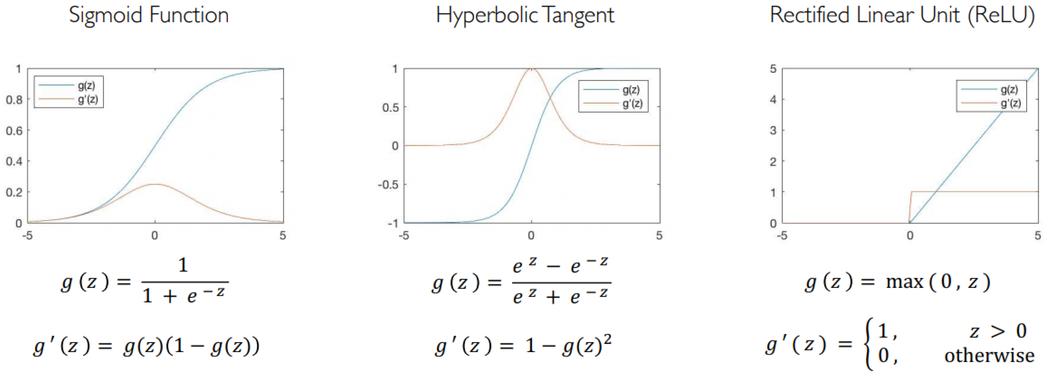
Mathematics 09 00968 g002
Figure 3. Common activation functions.
Mathematics 09 00968 g003
Figure 4. Scatter plot and correlation between variables by response for the breast cancer data.
Mathematics 09 00968 g004
Figure 5. Scatter plot and correlation between variables by response in heart disease data.
Mathematics 09 00968 g005
Figure 6. Scatter plot and correlation between variables by response in prostate cancer data.
Mathematics 09 00968 g006
Figure 7. Correlation between variables and PCA for the breast cancer data.
Mathematics 09 00968 g007
Figure 8. Variable PCA for the breast cancer data.
Mathematics 09 00968 g008
Figure 9. Breast cancer PCA bipot.
Mathematics 09 00968 g009
Figure 10. Lasso λ using 10 fold cross validation for the breast cancer data.
Mathematics 09 00968 g010
Figure 11. Ridge λ using 10 fold cross-validation for the breast cancer data.
Mathematics 09 00968 g011
Figure 12. Coefficients for our LR-lasso model for the breast cancer data. The dotted vertical line in the plot represents the λ with misclassification error (MCE) within one standard error of the minimum MCE.
Mathematics 09 00968 g012
Figure 13. Coefficients for our LR-ridge model for the breast cancer data. The dotted vertical line in the plot represents the λ with misclassification error (MCE) within one standard error of the minimum MCE.
Mathematics 09 00968 g013
Figure 14. Variables importance plot for lasso and ridge regression for the breast cancer data.
Mathematics 09 00968 g014
Figure 15. Selecting λ and the number of components using 10-fold cross-validation for the breast cancer data.
Mathematics 09 00968 g015
Figure 16. Selecting the number of components by CV for the breast cancer data.
Mathematics 09 00968 g016
Figure 17. Selecting the number of components by CV for the breast cancer data.
Mathematics 09 00968 g017
Figure 18. MARS variables importance plot for the breast cancer data.
Mathematics 09 00968 g018
Figure 19. Selecting the split size.
Mathematics 09 00968 g019
Figure 20. Selecting the tree size for the breast cancer data.
Mathematics 09 00968 g020
Figure 21. RF important variables in predicting breast cancer.
Mathematics 09 00968 g021
Figure 22. Selecting the tree size for the breast cancer data.
Mathematics 09 00968 g022
Figure 23. GBM important variables for the breast cancer data.
Mathematics 09 00968 g023
Figure 24. Selecting the cost parameter for the breast cancer data.
Mathematics 09 00968 g024
Figure 25. SVM important variables for the breast cancer data.
Mathematics 09 00968 g025
Figure 26. FFNN important variables for the breast cancer data.
Mathematics 09 00968 g026
Figure 27. RF for the breast cancer data.
Mathematics 09 00968 g027
Table 1. Name of variables and description for the heart disease data.
VariableDescription
IdSample code number
I Cl.thicknessClump Thickness
Cell.sizeUniformity of Cell Size
Cell.shapeUniformity of Cell Shape
Marg.adhesionMarginal Adhesion
Epith.c.sizeSingle Epithelial Cell Size
Bare.nucleiBare Nuclei
Bl.cromatinBland Chromatin
Normal.nucleoliNormal Nucleoli
MitosesMitoses
ClassClass
Table 2. % of variation explained by each component for the breast cancer data.
STATISTICSPC1PC2PC3PC4PC5PC6PC7PC8PC9
Std deviation2.430.880.730.680.620.550.540.510.30
Prop of Variance0.660.090.060.050.040.030.030.030.01
Cum Proportion0.660.740.800.850.890.930.960.991.00
Table 3. Coefficient, prediction accuracy of lasso and ridge LR model for the breast cancer data.
FeaturesLR-Ridge CoefficientLR-Lasso Coefficient
Cl.thickness0.17121770.23606
Cell.size0.12537540.07934
Cell.shape0.14348340.18897
Marg.adhesion0.11409870.05437
Epith.c.size0.1267267NA
Bare.nuclei0.14219010.20966
Bl.cromatin0.18046710.2299
Normal.nucleoli0.11153920.08242
Mitoses0.1274586NA
Pred. Accuracy0.97560.9659
Table 4. Coefficient of principal components for the breast cancer data.
EstimateStd. Errorz Valuep-Value
(Intercept)−1.2630.3278−3.8530.00011
PC1−2.27080.2597−8.7460.00000
PC20.14890.3870.3850.07302
PC30.77540.39231.9770.04809
Null deviance = 617.334 on 477 df and Residual deviance = 85.926 on 474 df AIC: 93.926 and Pred. Accuracy: 0.9707.
Table 5. Selecting the optimal model for FFNN using misclassification error for the breast cancer data.
Actva.EpochsHiddenIDRL1L2L.RateMiss.Err
Maxout100[9,3,2]0.0508e-054e-050.0200.006
Maxout100[5,5,2]0.0009e-058e-050.0100.015
Maxout100[9,2]0.0002e-051e-020.0100.015
Maxout50[9,3,2]0.0003e-055e-050.0200.015
Maxout100[9,2]0.0009e-052e-020.0200.015
Table 6. All models applied to the breast cancer data.
ModelSensitivitySpecificityAccuracy (95% CI)
LR-Ridge0.97240.94520.9656 (0.9440, 0.9920)
LR-Lasso0.98480.93150.9659 (0.9309, 0.9862)
LR-Enet0.98480.94520.9707 (0.9374, 0.9892)
LR-PC0.98480.94520.9707 (0.9374, 0.9892)
LR-PLS0.97730.93150.9610 (0.9246, 0.9830)
MARS0.95890.96210.9610 (0.9246, 0.9830)
SVM0.98480.95890.9756 (0.9440, 0.9920)
RF0.97730.97260.9756 (0.9440, 0.9920)
GBM0.97730.95890.9707 (0.9374, 0.9892)
FFNN0.94730.99200.97561 (0.9309, 0.9862)
Table 7. % variation explained by each component for the heart disease data.
PC1PC2PC3PC4PC5PC6PC7PC8PC9
Std Dev1.761.271.121.051.000.930.920.880.83
Prop. var0.240.120.100.090.080.070.060.060.05
Cum. Prop.0.240.360.460.540.620.690.750.810.86
Table 8. % variation explained by each components for the prostate cancer data.
PC1PC2PC3PC4PC5PC6PC7PC8
Std. Dev.1.871.280.930.780.680.650.570.40
Prop. Var.0.440.210.110.080.060.050.040.02
Cum. Prop.0.440.640.750.830.890.940.981.00
Table 9. Comparing predictive performance of the 10 models applied to the heart disease data.
ModelSensitivitySpecificityAccuracy (95% CI)
LR-Ridge0.95650.73580.8384 (0.7509, 0.9047)
LR-Lasso0.97830.67920.8182 (0.7280, 0.8885)
LR-Enet0.95650.73580.8384 (0.7509, 0.9047)
LR-PC0.95650.73580.8384 (0.7509, 0.9047)
LR-PLS0.95650.73580.8384 (0.7509, 0.9047)
MARS0.60380.89130.7374 (0.6393, 0.8207)
SVM0.95650.73580.8384 (0.7509, 0.9047)
RF0.91300.69810.7980 (0.7054, 0.872)
GBM0.93480.73580.8283 (0.7394, 0.8967)
FFNN0.80000.87000.8383 (0.7475, 0.8817)
Table 10. Comparing predictive performance of the 10 models applied to the prostate cancer data.
ModelSensitivitySpecificityAccuracy (95% CI)
LR-Ridge0.75000.90480.8485 (0.681, 0.9489)
LR-Lasso1.00001.00001.0000 (0.8942, 1.0000)
LR-Enet1.00001.00001.0000 (0.8942, 1.0000)
LR-PC0.91671.00000.9697 (0.8424, 0.9992)
LR-PLS0.83330.80950.8182 (0.6454, 0.9302)
MARS1.00001.00001.0000 (0.8942, 1.0000)
SVM0.91670.76190.8182 (0.6454, 0.9302)
RF1.00001.00001.0000 (0.8942, 1.0000)
GBM1.00001.00001.0000 (0.8942, 1.0000)
FFNN0.90910.90910.9091 (0.7567, 0.9808)
Table 11. Performance assessment of the 10 models for the breast cancer data.
ModelSpecificitySens/RecallPrecisionROC-AUCPR-AUC
LR-Ridge0.94520.97240.98570.99770.9825
LR-Lasso0.93150.98480.97140.99780.9825
LR-Enet0.94520.98480.97180.99780.9823
LR-PC0.94520.98480.97180.99700.9816
LR-PLS0.93150.97730.98550.99490.9836
RF0.97260.97730.95950.99840.8126
GBM0.95890.97730.95890.99580.9798
MARS0.96210.95890.93330.99010.9723
SVM0.95890.98480.93510.98830.9546
FFNN0.99200.94730.97300.99820.9832
Publisher’s Note: MDPI stays neutral with regard to jurisdictional claims in published maps and institutional affiliations.

