Abstract
In this paper, we study a monotone inclusion problem in the framework of Hilbert spaces. (1) We introduce a new modified Tseng’s method that combines inertial and viscosity techniques. Our aim is to obtain an algorithm with better performance that can be applied to a broader class of mappings. (2) We prove a strong convergence theorem to approximate a solution to the monotone inclusion problem under some mild conditions. (3) We present a modified version of the proposed iterative scheme for solving convex minimization problems. (4) We present numerical examples that satisfy the image restoration problem and illustrate our proposed algorithm’s computational performance.
1. Introduction
Let H be a real Hilbert space with the inner product and induced norm . A zero-point problem for monotone operators is defined as follows: find such that
where T is a monotone operator. Barely a decade ago, many authors intensively studied the convergence of iterative methods to find a zero-point for monotone operators in the framework of Hilbert spaces. Additionally, many iterative methods have been constructed and studied to solve a zero-point problem (1), since it is connected to various optimization and nonlinear analysis issues, such as variational inequality problems, convex minimization problems, and so on. The proximal point algorithm (PPA) [1], which was constructed by Martinet in 1970, is well known as being the first algorithm to solve the problem (1). This algorithm is shown below:
where I is the identity mapping, and is a sequence of positive real numbers. After Martinet [1] proposed the proximal point algorithm (PPA), many algorithms were developed by many authors to solve the zero-point problem. The reader can see [2,3,4] and the references therein for more details.
In this paper, we focus on the following monotone inclusion problem:
where and are single and multi-valued mappings, respectively. The monotone inclusion problem (3) can be written as the zero-point problem (1) by setting . However, the full resolvent operator is much harder to compute than the resolvent operators and .
Because the monotone inclusion problem (3) is the core of image processing and many mathematical problems [5,6,7,8,9,10,11,12,13,14,15,16,17,18,19,20,21,22], many researchers have proposed and developed iterative methods for solving inclusion problems (3). The forward-backward splitting method, constructed and studied by Lions and Mercier [23] in 1979, is the most popular algorithm for solving the (3) problem. It is defined by the following iterative:
where is arbitrarily chosen and . In the algorithm (4), operators A and B are usually called the forward operator and the backward operator, respectively. For more details about forward-backward methods that have been constructed and considered to solve the inclusion problem (3), the reader is directed to [2,9,11,24,25,26,27,28,29,30,31,32].
To speed up the convergence rate of iteration methods, Polyak [33] introduced inertial extrapolation as an acceleration process in 1964. This method is well known as the heavy ball method. Polyak [33] used his algorithm to solve the smooth convex minimization problem. In recent years, many researchers have intensively used this useful concept for combining their algorithms with an inertial term to accelerate the speed of convergence.
In 2001, Alvarez and Attouch [34] constructed an algorithm to solve a problem of monotone operators. It combines the heavy ball method with the proximal point algorithm. The algorithm is defined as follows:
where are arbitrarily chosen, , and is nondecreasing with
They proved that the sequence generated by the algorithm (5) converges weakly to a zero-point of the monotone operator B.
Moudafi and Oliny [35] studied the monotone inclusion problem (3). They constructed the inertial proximal point algorithm, which combines the heavy ball method with the proximal point algorithm. The inertial proximal point algorithm is defined as follows:
where are arbitrarily chosen, and and are single and multi-valued mappings, respectively. It was proven that if with the Lipschitz constant L of the monotone operator A and the condition (6) holds, then the sequence generated by the algorithm (7) converges weakly to a solution of the inclusion problem (3). Moreover, it has been observed that for , the proximal point algorithm (7) cannot be written as the forward-backward splitting method (4), since there is no estimation of operator A at point .
Lorenz and Pock [36] studied the monotone inclusion problem (3). They proposed the inertial forward-backward algorithm for monotone operators, which is defined as
where are arbitrarily chosen, and are single and multi-valued mappings, respectively. They proved that the sequence generated by the algorithm (8) converges weakly to a solution of the monotone inclusion problem (3) with some conditions.
Kitkuan and Kumam [26] combined the forward-backward splitting method (4) with the viscosity approximation method [37] for solving the monotone inclusion problem (3). It is called the inertial viscosity forward-backward splitting algorithm, which is defined as:
where are arbitrarily chosen, is a differentiable function such that its gradient is a contraction with the constant , and and are an inverse strongly monotone and a maximal monotone operator, respectively. They proved that the sequence generated by the algorithm (9) converges strongly to a solution of the monotone inclusion problem (3) under suitable conditions.
Besides solving the monotone inclusion problem using an algorithm combined with the heavy ball idea, there are many ways to solve the monotone inclusion problem. Tseng [24] introduced a powerful iterative method to solve the monotone inclusion problem (3), which is called the modified forward-backward splitting method. In short, it is known as Tseng’s splitting algorithm. Let C be a closed and convex subset of a real Hilbert space H. Tseng’s splitting algorithm is defined as
where is arbitrarily chosen, is chosen to be the largest satisfying where , , and is the projection onto a closed convex subset C of H. However, Tseng’s splitting algorithm only obtains weak convergence in real Hilbert spaces.
Recently, Dilshad, Aljohani, and Akram [38] introduced and studied an iterative scheme to approximate the common solution to a split variational inclusion and a fixed-point problem of a finite collection of nonexpansive mappings. Let and be two real Hilbert spaces and be a bounded linear operator with its adjoint operator . Their algorithm is
where is arbitrarily chosen, , , f is a contraction with a constant , and is a finite collection of nonexpansive mappings. For more detail about the split variational inclusion in other class of mappings and methods for solving them, the reader is directed to [39,40,41,42].
Based on the above idea, we introduce a new modified Tseng’s method, which combines inertial and viscosity techniques to solve inclusion problems in the framework of real Hilbert spaces. The project aims to obtain algorithms with better performance and can be applied for a broader class of mappings. Furthermore, we present a modified version of the proposed iterative scheme to solve convex minimization problems. Moreover, we illustrate the computational performance of our proposed algorithms by conducting experiments that satisfy the image restoration problem.
2. Preliminaries
In this section, we present some notations that are used throughout this work. Let H be a real Hilbert space with the inner product and the induced norm . Let C be a nonempty closed and convex subset of a real Hilbert space H. and denote the strong convergence and weak convergence of a sequence to . For any point x, there exists a unique nearest point for C, which is denoted by , such that for all . The operator denotes the metric projection from H onto C. It is well known that the metric projection is nonlinear, and it satisfies the following:
for all . Next, we present several properties of operators and set-valued mappings, which are helpful later. Let be a mapping, denotes the set of fixed points of T, i.e.,
Proposition 1.
Let H be a real Hilbert space and be a mapping.
- 1.
- T is callednonexpansive mappingiffor all
- 2.
- T is called firmly nonexpansive mapping iffor all
Proposition 2
([43]). Let be a mapping. Then, the following items are equivalent:
- (i)
- T is firmly nonexpansive;
- (ii)
- is firmly nonexpansive;
- (iii)
- for all
It is well known that the metric projection is a firmly nonexpansive mapping, i.e.,
for all
For convenience, we let be a set-valued mapping and
be the resolvent of mapping B where . It is well known that is single-valued, , where is a domain of the operator , and is a firmly nonexpansive mapping for all .
Definition 1.
Let be a set-valued mapping with the graph . B is called monotone if,
for all and . A monotone mapping is maximal if the graph of for B is not properly contained in the graph of any other monotone mapping.
Definition 2
([44]). Let be a mapping.
- 1.
- T is called L-Lipchitz continuous if a non-negative real number exists such thatfor all .
- 2.
- T is called α-inverse strongly monotone if a positive real number α exists such thatfor all . Moreover, if T is α-inverse strongly monotone, then T is -Lipschitz continuous.
Lemma 1
([43]). Let H be a real Hilbert space. Then, the following equations hold:
- (i)
- , for all ;
- (ii)
- , for all ;
- (iii)
- for all and
Lemma 2
([45]). Let H be a real Hilbert space. Let be an α-inverse strongly monotone operator and be a maximal monotone operator. Then, for , the following relation holds:
Lemma 3
([46]). Let be a sequence of non-negative real numbers that satisfy the following relation:
where
- (i)
- (ii)
- (iii)
Then, as
Lemma 4
([47]). Let be sequence of real numbers that does not decrease at infinity in the sense that the following subsequence exists: of such that for all . Additionally, consider the sequence of integers defined by
Then is a nondecreasing sequence that verifies and for all
3. Results
In this section, we present a convergence analysis of the proposed algorithm, which generates sequences that converge strongly to a solution to the monotone inclusion problem (3). Throughout this section, is used to denote the set of all the solutions to the monotone inclusion problem (3). We use the following conditions for the analysis of our method.
Assumption 1.
- A1
- Ω is nonempty.
- A2
- A is L-Lipschitz continuous and monotone, and B is maximal monotone.
- A3
- is σ-Lipschitz continuous, where
- A4
- Let be a sequence in such that and .
Remark 1.
Observe that from Assumption 1 (A4) and Algorithm 1, we have from that
- (1)
- .
- (2)
- .
| Algorithm 1 An iterative algorithm for solving inclusion problems |
| Initialization: Given , . Let be arbitrary. Choose , to satisfy Assumption 1 and to satisfy Remark 1. Iterative Step: Given the current iterate , calculate the next iterate as follows: Step 1. Compute Step 2. Update Replace n with and then repeat Step 1. |
Next, we provide a useful lemma for analyzing our main theorem.
Lemma 5
([11]). The sequence generated by (14) is a non-increasing sequence and
Lemma 6
([11]). Assume that Assumption (1) holds and let be any sequence generated by Algorithm 1. Then,
for all and
Theorem 1.
Assume that Assumptions (1) A1–A4 hold. Let be a sequence generated by Algorithm 1. Then, , where
Proof.
Step 1. We prove that , , and are bounded sequences. Assume that Since [11]
and
Moreover, we observe that
and
Consider
Thus, is bounded and , , and are bounded.
Next, we observe that
It follows that
and
Then, by combining (22) with (23), we find that
Next, by combining (17) with the above inequality, we find that
Consider
It follows that
Therefore, we obtain
Moreover, by using (26), we obtain
Next, we consider two possible cases to show that .
Case 1. Suppose that the sequence is non-increasing, exists such that for each . Therefore, converges.
Since , , by using Remark 1, we obtain from (27) that
Thus, from (18), we immediately obtain
If we consider
then
Since is bounded, take a subsequence of such that . By setting , we have
Using the fact that and (29), we obtain
Therefore, . We can obtain
By applying Lamma 3 and using (28) and (35) and using conditions of all parameters, we can claim that
Case 2. Suppose that the sequence is increasing. Let be a mapping for all values (where N is large enough). This is defined by
Then, as and for all . By using (27), and the conditions of the parameters for each , we have
Since , we can conclude that
Moreover, by following the proof in Case 1, we obtain
Using (28), we have
By applying Lamma 3 to (39), using (38) and the conditions of all parameters, we can claim that
Using Lemma 4, we obtain
Therefore, which completes the proof. □
4. Applications and Numerical Results
Let and be a convex function and a convex, lower-semicontinuous, and nonsmooth function, respectively. Consider the convex minimization problem that finds such that
Using Fermat’s rule, an equivalent of the problem (41) is obtained in the form
where is a subdifferential of G, which is a maximal monotone. For more detail, we direct the reader to [48]. is a gradient of F, which is -Lipschitz continuous [49]. By setting and , we obtain the following theorem:
| Algorithm 2 An iterative algorithm for solving the convex minimization problems |
| Initialization: Given , , let be arbitrary. Choose , to satisfy Assumption 1 and to satisfy Remark 1. Iterative Step: Given the current iterate , calculate the next iterate as follows: Step 1. Compute Step 2. Update Replace n with and then repeat Step 1. |
Theorem 2.
Assume that Assumptions (1) A1–A4 are held. Let be a sequence generated by Algorithm 2. Then, , where
In this paper, we focus on the topic of image restoration. The inversion of the following model can be used to formulate the image restoration problem:
where is an original image, is the observed image, b is additive noise, and . To solve the problem (43), we can transform it into the least squares minimization problem
where is a regularization parameter. We set , and . The Lipschitz gradient of F is in the form
where is a transpose of operator A. Now, an iteration is used to find the solution to the following convex minimization problem: Find such that
where A is a bounded linear operator and b is the degraded image. Therefore, we use Theorem 2 to solve (45) by setting , and . Next, since , we immediately know from [50] that
In this part, we present the restoration of an image that has been corrupted by a motion blur specified by a motion length of 22 pixels and a motion orientation of 45 (blur matrix ), a Gaussian blur with a filter size of and a standard deviation of (blur matrix ), an out of focus blur or a circular average filtered blurred image with a radius of (blurred matrix ), and an average blur with a filter size of (blurred matrix ), respectively. We use Algorithm 2 to restore the original grey (cameraman) and RGB (baboon) images, which are shown in Figure 1. Blurred grey images and blurred RGB images with a blurred matrix – are shown in Figure 2 and Figure 3, respectively.
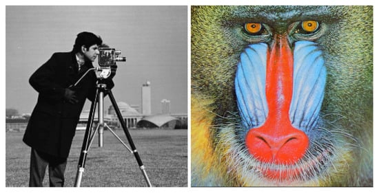
Figure 1.
Original images.

Figure 2.
Blurred grey images with blurred matrixes –, respectively.

Figure 3.
Blurred RGB images with blurred matrixes –, respectively.
The reconstructed grey images corrupted by blurred matrixes – are shown in Figure 4, and the reconstructed RGB images corrupted by blurred matrixes – are shown in Figure 5.

Figure 4.
Reconstructed grey images corrupted by blur matrixes –, respectively.
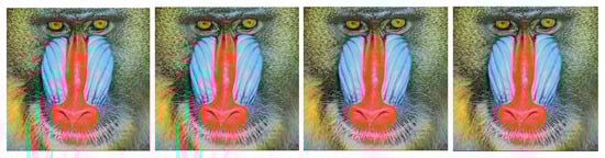
Figure 5.
Reconstructed RGB images corrupted by blurred matrixes –, respectively.
In order to measure the quality of the restored images, we use the signal-to-noise ratio:
where x is an original image. The behavior of SNR for the Algorithm 2 of all cases for grey and RGB images are shown in Figure 6 and Figure 7, respectively.
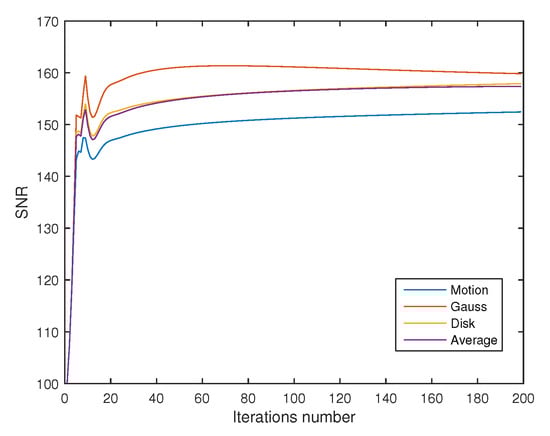
Figure 6.
The behavior of SNR for the Algorithm 2 of all cases for grey images.
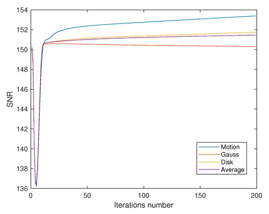
Figure 7.
The behavior of SNR for the Algorithm 2 of all cases for RGB images.
5. Conclusions
In this paper, we proposed a modified Tseng’s method that combines inertial and viscosity techniques to solve monotone inclusion problems in real Hilbert spaces. We also established a strong convergence theorem. Our modifications improve the practicality of the algorithm, which means that it performs better and can be applied for a more expansive mapping class. Moreover, we used our algorithm to solve some parts of image recovery problems.
Author Contributions
N.K. and K.S. contributed equally in writing this article. All authors have read and agreed to the published version of the manuscript.
Funding
This research was funded by Thailand Science Research and Innovation Fund, and King Mongkut’s University of Technology North Bangkok with Contract no. KMUTNB-BasicR-64-33-1.
Acknowledgments
The authors would like to thank the Department of Mathematics, Faculty of Applied Science, King Mongkut’s University of Technology North Bangkok.
Conflicts of Interest
The authors declare no conflict of interest.
References
- Martinet, B. Régularisation d’inéquations variationnelles par approximations successives. Rev. Française Informat. Recherche Opérationnelle 1970, 4, 154–158. [Google Scholar]
- Rockafellar, R.T. Monotone operators and the proximal point algorithm. SIAM J. Control Optim. 1976, 14, 877–898. [Google Scholar] [CrossRef]
- Reich, S. Extension problems for accretive sets in Banach spaces. J. Funct. Anal. 1977, 26, 378–395. [Google Scholar] [CrossRef]
- Nevanlinna, O.; Reich, S. Strong convergence of contraction semigroups and of iterative methods for accretive operators in Banach spaces. Isr. J. Math. 1979, 32, 44–58. [Google Scholar] [CrossRef]
- Combettes, P.L.; Wajs, V.R. Signal recovery by proximal forward-backward splitting. Multiscale Model. Simul. 2005, 4, 1168–1200. [Google Scholar] [CrossRef]
- Byrne, C. A unified treatment of some iterative algorithms in signal processing and image reconstruction. Inverse Probl. 2003, 20, 103. [Google Scholar] [CrossRef]
- Byrne, C. Iterative oblique projection onto convex sets and the split feasibility problem. Inverse Probl. 2002, 18, 441. [Google Scholar] [CrossRef]
- Hanjing, A.; Suantai, S. A fast image restoration algorithm based on a fixed point and optimization method. Mathematics 2020, 8, 378. [Google Scholar] [CrossRef]
- Thong, D.V.; Cholamjiak, P. Strong convergence of a forward–backward splitting method with a new step size for solving monotone inclusions. Comput. Appl. Math. 2019, 38, 1–16. [Google Scholar] [CrossRef]
- Marcotte, P. Application of Khobotov’s algorithm to variational inequalities and network equilibrium problems. INFOR Inf. Syst. Oper. Res. 1991, 29, 258–270. [Google Scholar] [CrossRef]
- Gibali, A.; Thong, D.V. Tseng type methods for solving inclusion problems and its applications. Calcolo 2018, 55, 1–22. [Google Scholar] [CrossRef]
- Khobotov, E.N. Modification of the extra-gradient method for solving variational inequalities and certain optimization problems. USSR Comput. Math. Math. Phys. 1987, 27, 120–127. [Google Scholar] [CrossRef]
- Kinderlehrer, D.; Stampacchia, G. An Introduction to Variational Inequalities and Their Applications; Society for Industrial and Applied Mathematics: Philadelphia, PA, USA, 2000. [Google Scholar]
- Trémolières, R.; Lions, J.L.; Glowinski, R. Numerical Analysis of Variational Inequalities; Elsevier: Amsterdam, The Netherlands, 2011. [Google Scholar]
- Konnov, I.V. Combined relaxation methods for variational inequality problems over product sets. Lobachevskii J. Math. 1999, 2, 3–9. [Google Scholar]
- Baiocchi, C. Variational and quasivariational inequalities. In Applications to Free-Boundary Problems; Wiley: New York, NY, USA, 1984. [Google Scholar]
- Jaiboon, C.; Kumam, P. An extragradient approximation method for system of equilibrium problems and variational inequality problems. Thai J. Math. 2012, 7, 77–104. [Google Scholar]
- Kumam, W.; Piri, H.; Kumam, P. Solutions of system of equilibrium and variational inequality problems on fixed points of infinite family of nonexpansive mappings. Appl. Math. Comput. 2014, 248, 441–455. [Google Scholar] [CrossRef]
- Chamnarnpan, T.; Phiangsungnoen, S.; Kumam, P. A new hybrid extragradient algorithm for solving the equilibrium and variational inequality problems. Afr. Mat. 2015, 26, 87–98. [Google Scholar] [CrossRef]
- Deepho, J.; Kumam, W.; Kumam, P. A new hybrid projection algorithm for solving the split generalized equilibrium problems and the system of variational inequality problems. J. Math. Model. Algorithms Oper. Res. 2014, 13, 405–423. [Google Scholar] [CrossRef]
- ur Rehman, H.; Kumam, P.; Cho, Y.J.; Yordsorn, P. Weak convergence of explicit extragradient algorithms for solving equilibirum problems. J. Inequalities Appl. 2019, 2019, 1–25. [Google Scholar] [CrossRef]
- Peters, J.F. Foundations of Computer Vision: Computational Geometry, Visual Image Structures and Object Shape Detection; Springer: Berlin, Germany, 2017; Volume 124. [Google Scholar]
- Lions, P.L.; Mercier, B. Splitting algorithms for the sum of two nonlinear operators. SIAM J. Numer. Anal. 1979, 16, 964–979. [Google Scholar] [CrossRef]
- Tseng, P. A modified forward-backward splitting method for maximal monotone mappings. SIAM J. Control Optim. 2000, 38, 431–446. [Google Scholar] [CrossRef]
- Kitkuan, D.; Kumam, P.; Martínez-Moreno, J. Generalized Halpern-type forward–backward splitting methods for convex minimization problems with application to image restoration problems. Optimization 2020, 69, 1557–1581. [Google Scholar] [CrossRef]
- Kitkuan, D.; Kumam, P.; Martínez-Moreno, J.; Sitthithakerngkiet, K. Inertial viscosity forward–backward splitting algorithm for monotone inclusions and its application to image restoration problems. Int. J. Comput. Math. 2020, 97, 482–497. [Google Scholar] [CrossRef]
- Huang, Y.; Dong, Y. New properties of forward–backward splitting and a practical proximal-descent algorithm. Appl. Math. Comput. 2014, 237, 60–68. [Google Scholar] [CrossRef]
- Goldstein, A.A. Convex programming in Hilbert space. Bull. Am. Math. Soc. 1964, 70, 709–710. [Google Scholar] [CrossRef]
- Padcharoen, A.; Kitkuan, D.; Kumam, W.; Kumam, P. Tseng methods with inertial for solving inclusion problems and application to image deblurring and image recovery problems. Comput. Math. Methods 2020, 3, e1088. [Google Scholar] [CrossRef]
- Attouch, H.; Peypouquet, J.; Redont, P. Backward–forward algorithms for structured monotone inclusions in Hilbert spaces. J. Math. Anal. Appl. 2018, 457, 1095–1117. [Google Scholar] [CrossRef]
- Dadashi, V.; Postolache, M. Forward–backward splitting algorithm for fixed point problems and zeros of the sum of monotone operators. Arab. J. Math. 2020, 9, 89–99. [Google Scholar] [CrossRef]
- Suparatulatorn, R.; Khemphet, A. Tseng type methods for inclusion and fixed point problems with applications. Mathematics 2019, 7, 1175. [Google Scholar] [CrossRef]
- Polyak, B.T. Some methods of speeding up the convergence of iteration methods. Ussr Comput. Math. Math. Phys. 1964, 4, 1–17. [Google Scholar] [CrossRef]
- Alvarez, F.; Attouch, H. An inertial proximal method for maximal monotone operators via discretization of a nonlinear oscillator with damping. Set-Valued Anal. 2001, 9, 3–11. [Google Scholar] [CrossRef]
- Moudafi, A.; Oliny, M. Convergence of a splitting inertial proximal method for monotone operators. J. Comput. Appl. Math. 2003, 155, 447–454. [Google Scholar] [CrossRef]
- Lorenz, D.A.; Pock, T. An inertial forward-backward algorithm for monotone inclusions. J. Math. Imaging Vis. 2015, 51, 311–325. [Google Scholar] [CrossRef]
- Cholamjiak, P.; Suantai, S. Viscosity approximation methods for a nonexpansive semigroup in Banach spaces with gauge functions. J. Glob. Optim. 2012, 54, 185–197. [Google Scholar] [CrossRef]
- Dilshad, M.; Aljohani, A.; Akram, M. Iterative Scheme for Split Variational Inclusion and a Fixed-Point Problem of a Finite Collection of Nonexpansive Mappings. J. Funct. Spaces 2020, 2020, 3567648. [Google Scholar] [CrossRef]
- Abbas, M.; Ibrahim, Y.; Khan, A.R.; De la Sen, M. Split variational inclusion problem and fixed point problem for a class of multivalued mappings in CAT (0) spaces. Mathematics 2019, 7, 749. [Google Scholar] [CrossRef]
- De la Sen, M. Stability and convergence results based on fixed point theory for a generalized viscosity iterative scheme. Fixed Point Theory Appl. 2009, 2009, 314581. [Google Scholar] [CrossRef][Green Version]
- Sitthithakerngkiet, K.; Deepho, J.; Kumam, P. A hybrid viscosity algorithm via modify the hybrid steepest descent method for solving the split variational inclusion in image reconstruction and fixed point problems. Appl. Math. Comput. 2015, 250, 986–1001. [Google Scholar] [CrossRef]
- Pan, C.; Wang, Y. Generalized viscosity implicit iterative process for asymptotically non-expansive mappings in Banach spaces. Mathematics 2019, 7, 379. [Google Scholar] [CrossRef]
- Bauschke, H.H.; Combettes, P.L. Convex Analysis and Monotone Operator Theory in Hilbert Spaces; Springer: New York, NY, USA, 2011; Volume 408. [Google Scholar]
- Suwannaut, S.; Suantai, S.; Kangtunyakarn, A. The method for solving variational inequality problems with numerical results. Afr. Mat. 2019, 30, 311–334. [Google Scholar] [CrossRef]
- López, G.; Martín-Márquez, V.; Wang, F.; Xu, H.K. Forward-backward splitting methods for accretive operators in Banach spaces. Abstr. Appl. Anal. 2012, 2012, 109236. [Google Scholar] [CrossRef]
- Xu, H.K. Iterative algorithms for nonlinear operators. J. Lond. Math. Soc. 2002, 66, 240–256. [Google Scholar] [CrossRef]
- Maingé, P.E. Strong convergence of projected subgradient methods for nonsmooth and nonstrictly convex minimization. Set-Valued Anal. 2008, 16, 899–912. [Google Scholar] [CrossRef]
- Rockafellar, R. On the maximal monotonicity of subdifferential mappings. Pac. J. Math. 1970, 33, 209–216. [Google Scholar] [CrossRef]
- Baillon, J.B.; Haddad, G. Quelques propriétés des opérateurs angle-bornés etn-cycliquement monotones. Isr. J. Math. 1977, 26, 137–150. [Google Scholar] [CrossRef]
- Hale, E.T.; Yin, W.; Zhang, Y. A Fixed-Point Continuation Method for L1-Regularized Minimization with Applications to Compressed Sensing; CAAM TR07-07; Rice University: Houston, TX, USA, 2007; Volume 43, p. 44. [Google Scholar]
Publisher’s Note: MDPI stays neutral with regard to jurisdictional claims in published maps and institutional affiliations. |
© 2021 by the authors. Licensee MDPI, Basel, Switzerland. This article is an open access article distributed under the terms and conditions of the Creative Commons Attribution (CC BY) license (https://creativecommons.org/licenses/by/4.0/).