Abstract
A new statistical model of spatial distribution of observed galaxies is described. Statistical correlations are involved by means of Markov chain ensembles, whose parameters are extracted from the observable power spectrum by adopting of the Uchaikin–Zolotarev ansatz. Markov chain trajectories with the Lévy–Feldheim distributed step lengths form the set of nodes imitating the positions of galaxy. The model plausibly reproduces the two-point correlation functions, cell-count data and some other important properties. It can effectively be used in the post-processing of astronomical data for cosmological studies.
1. Introduction
One of the important aims of modern observational cosmology is the investigation of the galaxy distribution in the universe. The distribution at all redhsifts depends both on the initial conditions present in the early universe and the successive dynamical evolution of galaxies through smooth accretion and merger events. The luminous part of this matter appears to astronomers as a hierarchy of galaxies, clusters of galaxies, clusters of clusters of galaxies, etc. At present, the results are observations of different samples, such as the Lick Observatory Catalog, 2dF Galaxy Redshift Survey, 2dF100k Redshift Survey, Sloan Digital Sky Survey and others. To operate with this data, it is necessary to present this information in a form convenient for mathematical analysis. The most advanced schemes (statistical models) of this kind are formulated in terms of random point distributions. In the framework of this model, the position of each spatially unresolved galaxy is interpreted as a point in three-dimensional space, and any data sample can be subjected to a standard procedure to determine its properties. Despite the seeming simplicity of this test, even the question on the homogeneity of the spatial galaxy distribution, being fundamentally important for cosmology [1,2], has not yet reached a general consensus [2,3,4]. The situation changed after Mandelbrot introduced the concept of the fractal into circulation [5], which made it possible to speak of homogeneous inhomogeneity [6,7], preserving the basic cosmological principle of the coordinate system origin equivalence [1], or more strictly, replacing it by its weakened Mandelbrot’s version [5].
According to observations, the two point correlation function of galaxies has a power-law form, on scales from 0.01 to 10 Mpc with the slope and a scale factor Mpc [1]. For a long time it was assumed that is a characteristic measure of inhomogeneity, and beyond Mpc, the distribution of galaxies becomes homogeneous [2]. This means that
for the ensembles number of galaxies inside a sphere of radius R centered at any galaxy (the positive number D is called the fractal dimension). Such a relation naturally originates from the model of self-similar hierarchical clustering [4]. Transition to the outer region with Poissonian uniform distribution, where
violates the self-similarity. Such random point structures, fractal on small scales and homogeneous on large ones, were suggested to be called mesofractals [8]. The presence of a boundary region between the fractal and homogeneous parts of the mesofractal can play a decisive role in establishing the horizon of a representative (fair) sample.
To investigate this problem in the frame of the basic cosmological principle, stating the equality of all points in space when choosing the origin [1], Mandelbrot offered interpreting the left hand side of Equation (1) as the expected number of Markov chain nodes with the transition probability
This law sufficiently reproducing inverse-power correlations observed in spatial galaxy distribution, turned out to be rather awkward when computing multiple convolutions [2]. For this reason, V. Uchaikin introduced Lévy–Feldheim distributed vectors [9,10], more suitable for that aim. This model was analytically investigated, improved and numerically tested [8,11]. The last question, which remained open, was the determination of numerical parameters entering the transition probability in the Markov chain.
Here we discuss some methodological questions of this approach, relating to a new (Uchaikin–Zolotarev) approximation of the galaxy power spectrum and involving the Ornstein–Zernike equation in the problem under consideration.
The article is structured as follows. Section 2 introduces the basic statistical measures of spatial point distributions—correlation function and power spectrum and correlation function (Figure 1 and Figure 2 correspondingly). Figure 1 discovers a noticeable difference between the theoretical Harrison-Zel’dovich power spectrum and experimental data, Figure 2 demonstrates the experimental evidence of transition from fractal regime to homogeneous one on large scales. Section 3 provides a 4-parameter Uchaikin–Zolotarev approximation and a method for estimating its parameters from observational data. Table 1 and Figure 3, Figure 4, Figure 5, Figure 6, Figure 7 and Figure 8 demonstrate the high efficiency of this approximation. Section 4 presents the solution to the Ornstein–Zernike equation in the form of a Neumann series, which serves as a basis for Monte Carlo simulations. The first term of this series describes the statistical properties of a fractal cluster that appears in the vicinity of a node. In two successive Section 5 and Section 6),the moments of the number of objects in the cluster and the probability distributions reconstructed from them are demonstrated. The results are confirmed by Monte Carlo simulations and are in agreement with three popular models (thermodynamical, negative-binomial and lognormal). The probability distribution reveals the important property of the self-similarity (scaling) with respect to the mean cell count number. The last (7th) section summarizes conclusions.
2. Power Spectrum and Correlation Function
An important statistical measure of the large-scale structure of the Universe is the two-point correlation function [2], which determines the joint probability
of finding two galaxies in disjoint infinitesimal volumes and , placed at the distance , and is a mean number of galaxies per unite volume. Instead of , its Fourier transformation called the power spectrum is often used (as is commonly accepted in cosmography, the Universe is assumed to be periodic in some large rectangular parallelepiped of volume V; see for details [2], Sections 34 and 41).
where is 3d vector in the Fourier-space (in units of “waves per box”; physical wavelengths are Mpc/k).
There exist several approximations of power spectrum. The simplest of them is the Harrison–Zel’dovich (HZ) spectrum
is shown on Figure 1 as dashed line. Bounding the range of values of the parameter n from below ensures the convergence of the integral over the spectrum at long waves, i.e., for ([2], remark to formula (42.3)). The HZ spectrum describes the fluctuations generated in the framework of the canonical inflationary scenario [12,13].
As one can see from Figure 1, and from the other ones shown further, this two-parameter power function gives a rather rough representation of the spectrum. Moreover, the mismatch between it and the measured spectra turns out to be different for different data catalogs, and if it is necessary to use a general analytical approximation during processing, it should be flexible enough and have more parameters that are sensitive enough to changes in the input data. As shown by Peebles, the HZ spectrum yields the large-distance asymptotics power-type
with . Although it is commonly accepted that is close to 1.8, processing of various catalogs reveals a significant scatter of this parameter (from 1.15 to 2.99, see column in Table 1 of the review [7]).

Figure 1.
Power spectrum from the Lick Observatory catalog (dots with bars). The dashed line represents HZ spectrum with [14], the continuous one represents UZ spectrum with .
Figure 2 relates to the important area of distances around which there have been lively disputes for several decades, in which Einstein also took part at one time (see [3,6]). Currently, the shown behavior of the correlation function is interpreted as a transition from the scale of the fractal arrangement of galaxies to the scale of their uniform (homogeneous) distribution. V. Uchaikin suggested to use for such random point arrangements the term mesofractals [8]. It should be emphasized that the mesofractal is a homogeneous (in the statistical sense) structure, whose properties do not depend on the choice of the origin. It is only required that it coincides with one of the material points (galaxies) of the given set.

Figure 2.
The correlation functions for different samples calculated with different estimators [7]. The dashed line relates to the homogeneous part of the mesofractal, whereas the dotted line plots the fractal contribution.
The authors of review [7] listed some possible reasons for the observed deviation from the power-type law: “(1) Inconsistency of the theoretical model with the real universe, (2) misinterpretation of the observed events, (3) incorrectness of the mathematical processing of data. The most important of the assumptions used in a number of processing algorithms is the Poisson type of the spatial galaxy distribution. From a mathematical point of view, the inhomogeneous Poisson distribution admits the independence of disjoint regions, actually, we deal with only one object, which is the observable universe and we cannot verify the independence of the observed regions. Therefore, we have no rights to apply limit theorems of probability theory.” This motivates the further research in this direction.
The appropriate spectrum for the mesofractal random point set has been proposed by Uchaikin and Zolotarev in their book [10]. This UZ spectrum is represented in the form
where and are chosen in an appropriate way. To understand the origin of this approximator, perform the inverse Fourier transform of (5) and obtain the integral equation
with the kernel
being the Lévy–Feldheim isotropic density [10]. Formally, Equation (6) has been derived for the killed Markov chain ensemble in [9,10], and q is the trajectory survival probability: if , the trajectory contains infinite numbers of nodes, providing long-range correlations; if , it consists of only one (the first) node and describes the short-scale correlations (direct correlations, as they are called within molecular physics). When and we arrive at Mandelbrot’s model of unbounded continuous clustering hierarchy with spectrum
having the form of HZ spectrum.
To remedy the problems with equation solving, Peebles offered to lessen the spatial gradients on scales 30 hMpc to at least 300 hMpc. A simple way to do this is to suppose that there are many different random walks distributed uniformly at random through space as in the Neyman–Scott program. Individual chains cannot be infinitely long, because that would make the mean space density diverge; and Peebles suggests truncating these trajectories with some deterministic number of steps. UZ model uses a random mechanism of truncation including the survival probability, which led to OZ equation. Within the molecular physics, it is known as the Ornstein–Zernike equation. A specific interpretation the OZ formalism has been found in the cosmological large-structure problem [15]. It has the form of the equation in [16], relating to statistical mechanics, and can be solved by the Monte Carlo method.
The four parameters contained in the UZ approximator make it not only a flexible tool for more fine tuning the model, but give a basis for statistical simulation of such ensembles for investigation of reliability of various estimators effectiveness. It is useful to keep in mind that parameters A and c relate to scaling characteristics of inhomogeneities, whereas and q determine the fractal dimension in fractal-like regions and the size of such regions. Advantages of the UZ approximator over HZ can be seen in Figure 1 and look more convincing in the case of statistically poorer catalogs (Figure 6, Figure 7 and Figure 8).
3. Estimation of UZ Spectrum Parameters
Let us represent the power spectrum P in the form:
where
This property of linear proportionality of P and A will be used to optimize approximation to experimental data.

Figure 3.
The 2dFGRS (The 2dF Galaxy Redshift Survey) power spectrum from [6] (dots); the curve is UZ approximation.

Figure 4.
The 2dFGRS power spectrum from [6] convolved with the survey window function for a fiducial linear theory model (dots); the curve is UZ approximation.
Let , , be the wave numbers used for the approximation, be corresponding observational data at points P to be approximated and be approximated values.
where is an error function, and are input data values pairs.
In fact, does not depend on A. This is because of linearity of P with respect to A, as we can see in (8). Rearranging terms of we obtain
where and , are observational data at points to be approximated. This is a parabolic function with indeterminate A. As , the parabola is U-shaped with vertex
Thus,
Regressions were performed in MATLAB environment with function fminsearch. The numerical values of the parameters and comparison of the corresponding UZ approximations with the original experimental spectra are shown in Table 1 and Figure 1, Figure 2, Figure 3, Figure 4, Figure 5, Figure 6, Figure 7 and Figure 8. All represented cases demonstrate a good theoretical and agreement despite the very noticeable difference in the initial spectra. This fact reveals a kind of flexibility of this approximation, which makes it possible to distinguish the features of spectra close to each other. At the same time, the table shows that “good” (smooth) theoretical data in a wide range of wavenumbers are reproduced with an error that rarely exceeds a few percent. The data presented in the table and in the figures indicate that the UZ approximation has been successfully tested and may be recommended as a working tool for the large scale structures processing.

Table 1.
Uchaikin–Zolotarev spectrum approximation (5) applied to the data given in [6]. The columns represent the spectrum convolved with the survey window function for a fiducial linear theory model, . , , = 1.86527.
Table 1.
Uchaikin–Zolotarev spectrum approximation (5) applied to the data given in [6]. The columns represent the spectrum convolved with the survey window function for a fiducial linear theory model, . , , = 1.86527.
| k | (%) | k | (%) | ||||
|---|---|---|---|---|---|---|---|
| 0.010 | 2.36 | 2.21 | 6.8 | 0.090 | 7.07 | 6.92 | 2.2 |
| 0.014 | 2.29 | 2.33 | −1.7 | 0.094 | 6.66 | 6.46 | 3.1 |
| 0.018 | 2.19 | 2.28 | −3.9 | 0.099 | 6.19 | 6.07 | 2.0 |
| 0.022 | 2.09 | 2.18 | −4.1 | 0.103 | 5.84 | 5.75 | 1.6 |
| 0.026 | 1.98 | 2.05 | −3.4 | 0.107 | 5.53 | 5.48 | 0.9 |
| 0.030 | 1.87 | 1.90 | −1.6 | 0.111 | 5.23 | 5.24 | −0.2 |
| 0.034 | 1.76 | 1.75 | 0.6 | 0.115 | 4.96 | 5.03 | −1.4 |
| 0.038 | 1.65 | 1.62 | 1.8 | 0.119 | 4.70 | 4.82 | −2.5 |
| 0.042 | 1.55 | 1.50 | 3.3 | 0.123 | 4.46 | 4.61 | −3.2 |
| 0.046 | 1.45 | 1.40 | 3.6 | 0.127 | 4.24 | 4.39 | −3.4 |
| 0.050 | 1.35 | 1.32 | 2.3 | 0.131 | 4.03 | 4.18 | −3.6 |
| 0.054 | 1.26 | 1.24 | 1.6 | 0.135 | 3.84 | 3.97 | −3.3 |
| 0.058 | 1.18 | 1.17 | 0.8 | 0.139 | 3.66 | 3.77 | −2.9 |
| 0.062 | 1.10 | 1.11 | −0.9 | 0.143 | 3.49 | 3.58 | −2.5 |
| 0.066 | 1.03 | 1.05 | −1.9 | 0.147 | 3.33 | 3.40 | −2.1 |
| 0.070 | 9.68 | 9.85 | −1.7 | 0.151 | 3.18 | 3.25 | −2.1 |
| 0.074 | 9.07 | 9.21 | −1.5 | 0.155 | 3.04 | 3.11 | −2.2 |
| 0.078 | 8.51 | 8.57 | −0.7 | 0.169 | 2.62 | 2.73 | −4.0 |
| 0.082 | 7.99 | 7.97 | 0.2 | 0.185 | 2.22 | 2.36 | −5.9 |
| 0.086 | 7.51 | 7.43 | 1.1 |

Figure 5.
2dFGRS spectrum [17] (blue symbols) and its UZ approximation (dashed line) with , , , .

Figure 6.
2dFGRS spectrum [18] (red symbols) and its UZ approximation (dashed line) with , , , .

Figure 7.
2dFGRS spectrum [19] (orange symbols) and its UZ approximation (dashed line) with , , , .

Figure 8.
2dFGRS spectrum [19] (green symbols) and its UZ approximations. Dashed line is approximation with , , , ; Dash-dotted line is approximation with , , , . Observe the influence of parameter .
4. The OZ-Equation Solving
The positive function can be interpreted as the average density (concentration) of the number of nodes of the Markov chain with transition probability and survival probability q, modeling the positions of galaxies.
The integral
gives the mean number of all nodes of the particle trajectory including the final one. The function itself can be expressed by its Neumann’s series expansion
where
and
is the multiple convolution of the distribution density . Two algorithms of Monte Carlo simulation of random vector with probability density (7) are described in [10,20]. The specific properties of the Lévy–Feldheim convolutions [10] represent (16) as
For and , isotropic LF densities are expressed through elementary functions of :
and
5. Cell Counts: Moments and Probabilities
As claimed in [21], in order to satisfy the main cosmological principle (in its weakened form), one should simulate trajectories by pairs. Marking results relating to paired trajectories by open circles, and to single ones by filled circles, we represent the k-th factorial moment of the random cell count as
where
Taking into account that the difference between factorial and central moments decreases, as the latter increase, one can take for asymptotically large R
Here
and is the sphere of the radius centered at the origin of coordinates.
The moments of the normalized cell count (for a single trajectory) and (for a paired trajectory) do not depend on R as . As a result, the asymptotical probability distribution of can be written in the scaling form:
Here is the density of the distribution of variable Z having the moments:
determined via the coefficients Kn presented in Table 2. To estimate their accuracy, we put in brackets five Peebles’ values ([2] Section 59). Asterisk mark his data for α = 1.23.
Table 2.
The coefficients (18) for a single trajectory. The values in brackets were taken from [2] (values with asterisk are for ).
There exists a whole theory of recovery of a function from its moments, but fortunately, we meet a very simple case. Table 2 prompts us to check the relation
This relation is a characteristic property for gamma distribution
Actually, multiplying Equation (19) by and integrating the result over the positive semiaxis yields
The parameter of gamma distribution can be expressed in terms of the variance of Z:
This is a remarkable fact, not only providing a tool convenient for practically dealing with the cell-count fluctuations, but linking the phenomenological mesofractal model with such theoretical ones as thermodynamical, negative-binomial and lognormal ones [22].
There was also performed a Monte Carlo simulation of random trajectories with transition probabilities for . The point number count has been gathered inside the sphere of radius . The trajectory is broken when coming out the boundary of the sphere of the radius . As a result of simulation, the function and its moments for = 0.5, 1.0, 1.5 have been obtained. Figure 9 demonstrate results of the simulation for R = 0.05, 0.1 and 0.2, = 1.0. All the histograms are satisfactory described by the gamma distribution.
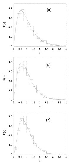
Figure 9.
Demonstration of the scaling of the probability density function for (a), 1.0 (b) and 1.5 (c). Full lines show gamma approximation histograms marking results of Monte Carlo simulations for three different values of R (0.05, 0.1 and 0.2).
Let emphasize that when dealing with a uniform Poissonian ensemble, we may center the count sphere at an arbitrary point of space, whereas in the fractal case, the center of the sphere must be chosen at a material point, i.e., at a galaxy (see [3,4,5]). The fluctuations of point number count inside the sphere (centered around any galaxy) do not vanish with increasing the radius but remain an essential value up to some distance where the transition domain begins.
6. Separation of Cluster and Background
At the end of this article, we return to the question concerning the fair–sample hypothesis. In particular, we discuss, whether a given catalog (or a part of it) is in a position to serve as a fair sample of galaxy statistics or not. Without making a final verdict, the following cautious considerations can be made on the basis of the model under consideration. It is easy to make sure that on large scales both conditional and unconditional statistics coincide and
Because the two-point function depends only on the distance r between the two points, it doesn’t matter where we put the origin of coordinate system. Therefore
and for simple (nonfactorial) moments of small orders we have:
and
where .
Remind that the last (fractal) terms of the moments (20) and (21), related in our interpretation to clusters, were calculated by Peebles [2] and represented in the form (formulas (60.7) and (60.13) of the cited book)
and
Factors were obtained from observation data and from some simple model offered by Peebles (we will denote them by ). The numerical results are presented in Table 3.
Table 3.
The moments for a paired trajectory. The lower values are results of Monte Carlo simulations.
Peebles noticed that his results are bounded by the condition because the variance
must be positive. At the same time, his formula (60.3) coincides with our formula (20) and both they yield the variance
being free from the defect. When
and
The two formulas are indication of the Poisson law. Consequently, there are reasons to suppose the galaxy distribution to be uniform at very large scales in accordance with the fair sample hypothesis, assuming uniformity of the Universe as a whole.
We end our article with demonstration of an artificial domain in the Universe, obtained by means of the trajectory ensemble with initially nods distributed according to uniform 3d Poisson process (Figure 10). Let us give a short explanation of how the image in Figure 10 appeared. Each point, representing a possible position of a galaxy (because its coordinate are random numbers, generated by computer, we call it artificial). For the sake of convenience, we picture points by means of open circles. when the dots condense, the circles overlap each other, darkened, or even completely black areas appear: these are clusters. Lévy–Feldheim distributions, have long power-law tails, and the remaining probability is concentrated in the region of small argument values. Observing the process of such wanderings on a large scale, we see how a wandering particle “tramples” for a long time in the vicinity of the starting point (generating an artificial galaxy with each hop) until a “long” run occurs, and the particle producing “galaxies” flights away from this places to create another cluster. We see such clusters in the figure. It remains only to add that the initial positions of the points are characterized by a uniform (in a statistical sense) distribution, there are no clusters, but descendants of these particles begin to appear, then particles of the next generation from them, and all this is superimposed on each other, reproducing the very hypothetical hierarchy of de Vaucouleur, and the result is a mesofractal: if you look closely, we will see clusters of different sizes, chaotically scattered over an almost uniform field of single particles depictured by filled circles. Nearby we placed the observed image (Figure 11) of one of clusters, taken from [7]. A comparison of these two pictures confirms our assumption that the set of point objects constructed by this method has a cluster character, explained by the peculiarity of the Lévy–Feldheim process [10].
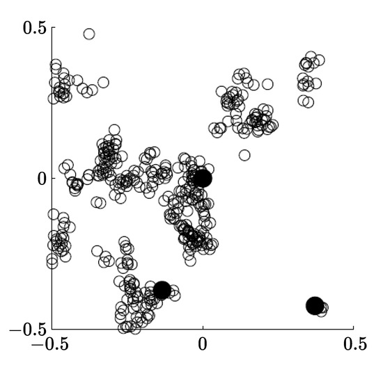
Figure 10.
2d projections of a domain with 700 artificial objects, simulated by means of the Monte Carlo method with .
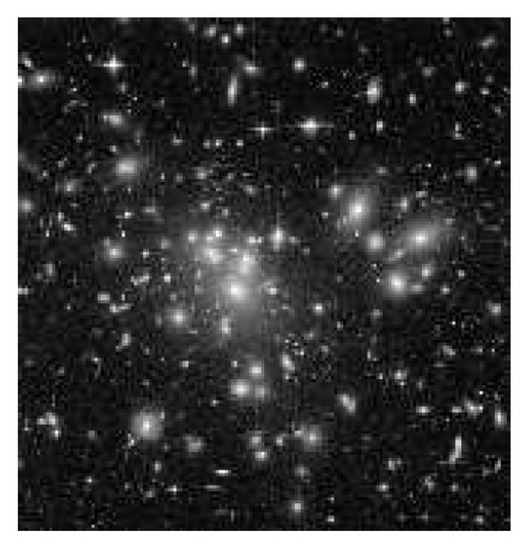
Figure 11.
The cluster of galaxies Abell 1689 at redshift seen by the HST with its recently installed Advanced Camera for Surveys (ACS) [7].
7. Conclusions
The aim of this work was to modify the Mandelbrot fractal model of point-like objects in 3d Euclidean space possessing properties similar to observed ones in the large scale galaxy distributions. In Mandelbrot’s model, the entire set of random points correlated according to the same (power) law as galaxies was generated by the nodes of a single random trajectory of an infinite Markov chain. The distances between successive nodes are distributed according to a power law, consistent with the characteristic of decreasing correlations in the observed samples. As the viewing radius increased, the statistics near the border worsened, and the question of what to expect beyond this statistical limit remained open. The present approach is based on a modification of this model: not a single infinite trajectory is considered, but a family of independent trajectories of a terminated Markov chain are, the initial nodes of which are distributed according to a uniform Poisson law in Euclidean space, and the distribution of distances between successive nodes of each of the trajectories corresponds to a 3d-stable isotropic Lévy–Feldheim law. The approach is based on a 4-parameter approximation of the experimentally observed spectrum, which has undergone extensive testing on data from several catalogs. A statistical analysis of the scheme built on these principles showed that the resulting arrangement of random point objects exhibits fractal properties on small scales, described in detail in the works of Mandelbrot, Peebles and Pietronero (see the list of references), and outside this area it continuously transforms into a uniform Poisson-type spatial distribution. The determination of the parameter values from the data on the power spectrum in the distribution of galaxies makes it possible to estimate the radius of such a sphere, beyond which the statistical distributions of galaxies can be considered mutually independent and the corresponding data can be used as a fair sample [2].
Author Contributions
Conceptualization, V.V.U.; Data curation, V.V.U.; Formal analysis, V.V.U. and V.A.L.; Project administration, E.V.K.; Software, I.I.K.; Visualization, E.V.K. and I.I.K.; Writing—original draft, V.V.U., V.A.L., E.V.K. and I.I.K.; Writing—review & editing, V.V.U. and V.A.L. All authors have read and agreed to the published version of the manuscript.
Funding
This research received no external funding.
Conflicts of Interest
The authors declare no conflict of interest.
References
- Weinberg, S. Gravitation and Cosmology; John Wiley and Sons, Inc.: Hoboken, NJ, USA, 1972. [Google Scholar]
- Peebles, P.J.E. The Large—Scale Structure of the Universe; Princeton University Press: Princeton, NJ, USA, 1980. [Google Scholar]
- Baryshev, Y.V.; Labini, F.; Montuori, M.; Pietronero, L. Facts and ideas in modern cosmology. Vistas Astron. 1994, 38, 419–500. [Google Scholar] [CrossRef]
- Coleman, P.H.; Pietronero, L. The fractal structure of the universe. Phys. Rep. 1992, 213, 311–389. [Google Scholar] [CrossRef]
- Mandelbrot, B.B. The Fractal Geometry of Nature; Freeman: New York, NY, USA, 1982. [Google Scholar]
- Cole, S.; Percival, W.J.; Peacock, J.A.; Norberg, P.; Baugh, C.M.; Frenk, C.S.; Baldry, I.; Bland-Hawthorn, J.; Bridges, T.; Cannon, R.; et al. The 2dF Galaxy Redshift Survey: Power-spectrum analysis of the final dataset and cosmological implications. Mon. Not. R. Astron. Soc. 2005, 362, 505–534. [Google Scholar] [CrossRef]
- Jones, B.J.; Martínez, V.J.; Saar, E.; Trimble, V. Scaling Laws in the Distribution of Galaxies. Rev. Mod. Phys. 2005, 76, 1211–1266. [Google Scholar] [CrossRef]
- Uchaikin, V.V. The mesofractal universe driven by Rayleigh-Lévy walks. Gen. Relativ. Gravit. 2004, 36, 1689–1718. [Google Scholar] [CrossRef]
- Uchaikin, V.V.; Gusarov, G.G. Lévy flight applied to random media problems. J. Math. Phys. 1997, 38, 2453–2464. [Google Scholar] [CrossRef]
- Uchaikin, V.V.; Zolotarev, V.M. Chance and Stability. Stable Distributions and Their Applications; VSP: Utrecht, The Netherlands, 1999. [Google Scholar]
- Uchaikin, V.V. If the Universe were a Lévy-Mandelbrot fractal. Gravit. Cosmol. 2004, 10, 5–24. [Google Scholar]
- Guth, A. Inflationary universe: A possible solution to the horizon and flatness problems. Phys. Rev. D 1981, 23, 347. [Google Scholar] [CrossRef]
- Linde, A. The inflationary Universe. Rep. Prog. Phys. 1984, 47, 925. [Google Scholar] [CrossRef]
- Fry, J.N. Gravity, Bias, and the Galaxy Three-Point Correlation Function. Phys. Rev. Lett. 1994, 73, 215–219. [Google Scholar] [CrossRef]
- Altenberger, A.R.; Dahler, D.S. On the galactic pair correlation function for a gravitational plasma. Astrophys. J. 1994, 421, L9–L12. [Google Scholar] [CrossRef]
- Stell, G. Statistical mechanics applied to random-media problems. Lect. Appl. Math. 1991, 27, 109–137. [Google Scholar]
- Percival, W.J.; Baugh, C.M.; Bland-Hawthorn, J.; Bridges, T.; Cannon, R.; Cole, S.; Colless, M.; Collins, C.; Couch, W.; Dalton, G.; et al. The 2dF Galaxy Redshift Survey: The power spectrum and the matter content of the Universe. Mon. Not. R. Astron. Soc. 2001, 327, 1297–1306. [Google Scholar] [CrossRef]
- Percival, W.J.; Burkey, D.; Heavens, A.; Taylor, A.; Cole, S.; Peacock, J.A.; Baugh, C.M.; Bland-Hawthorn, J.; Bridges, T.; Cannon, R.; et al. The 2dF Galaxy Redshift Survey: Spherical Harmonics analysis of fluctuations in the final catalogue. Mon. Not. R. Astron. Soc. 2004, 353, 1201–1220. [Google Scholar] [CrossRef]
- Tegmark, M.; Blanton, M.R.; Strauss, M.A.; Hoyle, F.; Schlegel, D.; Scoccimarro, R.; Vogeley, M.S.; Weinberg, D.H.; Zehavi, I.; Berlind, A.; et al. The Three-Dimensional Power Spectrum of Galaxies from the Sloan Digital Sky Survey. Astrophys. J. 2004, 606, 702–740. [Google Scholar] [CrossRef]
- Uchaikin, V.V.; Saenko, V.V. Simulation of random vectors with isotropic fractional stable distribution. J. Math. Sci. 2002, 112, 4211–4228. [Google Scholar] [CrossRef]
- Uchaikin, V.; Gismjatov, I.; Gusarov, G.; Svetukhin, V. Paired Lévy-Mandelbrot Trajectory as a Homogeneous Fractal. Int. J. Bifurc. Chaos 1998, 8, 977–984. [Google Scholar] [CrossRef]
- Messina, A.; Moscardini, L.; Lucchin, F.; Matarrese, S. Non-Gaussian initial conditions in cosmological N-body simulations. I-Space-uncorrelated models. Mon. Not. R. Astron. Soc. 1990, 245, 244–254. [Google Scholar]
Publisher’s Note: MDPI stays neutral with regard to jurisdictional claims in published maps and institutional affiliations. |
© 2021 by the authors. Licensee MDPI, Basel, Switzerland. This article is an open access article distributed under the terms and conditions of the Creative Commons Attribution (CC BY) license (http://creativecommons.org/licenses/by/4.0/).