Abstract
We introduce two families of continuous distribution functions with not-necessarily symmetric densities, which contain a parent distribution as a special case. The two families proposed depend on two parameters and are presented as an alternative to the skew normal distribution and other proposals in the statistical literature. The density functions of these new families are given by a closed expression which allows us to easily compute probabilities, moments and related quantities. The second family can exhibit bimodality and its standardized fourth central moment (kurtosis) can be lower than that of the Azzalini skew normal distribution. Since the second proposed family can be bimodal we fit two well-known data set with this feature as applications. We concentrate attention on the case in which the normal distribution is the parent distribution but some consideration is given to other parent distributions, such as the logistic distribution.
1. Introduction
There are many situations in which empirical data show slight or marked asymmetry. This is frequently the case, for example, with actuarial and financial data which, in addition to this feature, have heavy tails reflecting the existence of extreme values. The se features mean that the data can not be adequately modeled by the Gauss (or normal) distribution. Furthermore, bimodal distributions appear naturally in many different scenarios. For example, in certain disease patterns, as well as in certain cancer incidence curves. Behind the bimodality (and multimodality as well) of some cancer incidence curves, and their study, clinicians can improve their understanding of cancer, the development process as well as the potential characteristics that identify cancer and that separate a particular type of cancer of all other types. This occurs, for example, in cases where there are two peaks of occurrence per age. The se cancers include Kaposi’s sarcoma and Hodgkin’s lymphoma. The latter type of cancer has two peaks of occurrence: in young people adults and middle-aged adults. On the other hand, the normal skew distribution appears naturally in stochastic frontier analysis when a normal distribution is assumed to represent the noise or idiosyncratic component and a half-normal distribution to represent the inefficiency term, in the event that the researcher imposes inefficient behavior on all firms in the sample of interest. See, for instance [1]. Recently, [2] introduces (using a finite mixture model) the zero inefficiency stochastic frontier model which can accommodate the presence of both efficient and inefficient firms in the sample by appearing various bimodal scenarios. The refore, it seems plausible to try to obtain families of distributions that incorporate bias to the normal distribution but that at the same time are more versatile in the sense of being able to adapt to the bimodal scenario that appears in different situations.
Although there are various mechanisms to obtain skewed distributions from an initial that is not skewed, (Two well-known procedures that allow to generalize an initial probability distribution, symmetric or not, are those provided in the works of [3,4], among others). Our attention here will focus on the mechanism for this purpose introduced by [5], which enjoys an undoubted popularity and has been the subject of research in numerous works. Let g and G be, respectively, the probability density function (pdf) and the cumulative distribution function (cdf) of a symmetric distribution. A random variate Z is said to have a skew distribution if its pdf is given by
This family of distributions has been widely studied as an extension of the normal distribution by means of a shape parameter, , which accounts for the skewness. In this case g and G are replaced in Equation (1) by the pdf and cdf of the standard normal distribution and the resulting distribution is called the skew normal distribution. It should be pointed out that the function g does not have to be precisely the derivative of the cdf G to ensure that the pdf given in Equation (1) is a genuine pdf, although this case has not been studied in depth in the statistical literature. Following the notation provided in Reference [6] we denote the family of distributions given by , where and are the pdf and cdf of the standard normal distribution, respectively, by . Furthermore, when a random variable follows a skew normal distribution with location parameter and scale parameter we will write SN.
In this article, a new generalization of the family of skew distributions given in Equation (1) is proposed, which also includes the skew family of distributions of Azzalini as a particular case; that is, the expression (1). The methodology used is based on the combination of Azzalini’s proposal and a result provided by [7] which led us to add a new parameter to the family (1). Later, from this new family a second family, very similar to the first, is introduced. This new family of distributions can exhibit bimodality and its standardized fourth central moment (kurtosis) can be lower than the kurtosis of the Azzalini skew normal distribution (and can be positive or negative).
In recent decades, starting from Azzalini’s proposal, several generalizations and extensions of the skew-normal distribution have been introduced (see for example [8]). For multivariate extensions, see References [9,10,11], among others. The methods applied in the present paper can be considered as extensions and alternatives to the well-known skew-normal distribution (see [5,12]), whose properties (see [12,13]), and corresponding estimation [14] have been widely discussed. Other ways of obtaining skewed normal distributions have also been introduced, such as the one proposed by Reference [15], the Balakrishnan skew-normal density in Reference [16], the proposed model of Reference [17] and the generalized normal distribution in References [18,19,20], among others. For an exhaustive and comprehensive study of the skew-normal distribution, see the recent book by Reference [21].
The class of probability models proposed in the present paper can also be considered as alternatives or as approximations to the usual collective risk models in actuarial settings (see [22,23] among others). Data sets in these settings are typically skewed and the generalized models of the present paper expected to provide better fits than the standard models. In collective risk settings the right tail of the distribution is of considerable interest since the likelihood of large claims is of concern. In addition, the total claim distribution is of interest. Normal approximations are frequently resorted to when dealing with these variables. The use of more flexible generalized normal models can be expected to yield improvement.
The organization of this paper is as follows. The main result from which we constructed the two proposed families is shown in Section 2. Due to the importance that the normal distribution plays in numerous problems of applied statistics we dedicate a complete section, Section 3, to the study of this distribution. For this purpose, the pdf, which appears in closed form, is shown for the two families. We also give expressions for the mean, variance and the third and fourth standardized cumulant, to compare with their equivalents corresponding to the classical (Azzalini) skew normal distribution. In Section 4, the parameter estimation problem is studied. In order to obtain numerical solutions to the maximum likelihood (ML) estimation problem, suitable software has to be used. Multivariate extensions are described briefly in Section 5. Some examples and applications are described in Section 6. Finally, some conclusions are drawn and promising fields for further research are proposed in the last Section.
2. Main Results
We recall (see [24]) that if X and Y are independent and indentically distributed random variables with a finite fractional moment and if for all real , , then they are symmetric. Also, the following Theorem, which appears in [7], is required for the main result which will appear later.
Theorem 1.
(see [7]) Let G be the cdf of an arbitrary distribution that is symmetric about zero. The n,
Expression (2) in Reference [25] also establishes this assertion.
2.1. The First Family of Skew Distributions
The following result presents the key contribution of this work, consisting of proposing, given a family of symmetrical distributions, a more general family not necessarily symmetric that includes as a particular case the first family.
Theorem 2.
Let X and Y two random variables with symmetric cdf’s and and pdf’s and , respectively. The n,
represents a genuine pdf for and .
Proof.
Without loss of generality, asume that X and Y are independent random variables. Taking into account the fact that is symmetric and using the result provided in Theorem 1, we get
Hence the result. □
Expression (3) can instead be viewed in the following form related to an infinite mixture construction. Let , , and , be the cdf of a symmetric distribution with support in the real line. Suppose now that is random and follows a uniform distribution in the interval , then
is also a genuine cdf symmetric around zero. That is, . Now, Equation (3) is derived by taking into account the fact that is a genuine pdf. Another elegant way to see that Equation (3) defines a genuine pdf is to consider the argument given in Lemma 1 in [15]. That is, let . Now, we have that and since
we have that .
The results in the following proposition are readily verified and consequently are stated without proof.
Proposition 1.
For the density (3) the following results hold.
Because of Result in Proposition 1, an identifiability problem will arise in if we allow to assume both positive and negative values. To avoid this problem we can and will restrict to be non-negative when discussing inference for this model. Observe that establishes that when we get as a special case the well studied skew family of distributions appearing in References [5,12].
In most cases the density function (3) does not have a simple, closed form but it can be computed numerically. However, closed-form expressions for the pdf can be obtained for some specific choices of well-known distributions. For example, if we utilize the pdf and cdf of the logistic distribution with location parameter and scale parameter in (3), i.e., take and , respectively, then (3) becomes
On the other hand, combining the pdf of the standard normal distribution with the cdf of the logistic distribution we have, after applying (3) the new pdf
If in Equation (3), we use a normal pdf and a normal cdf, i.e., take and , where and represent the pdf and cdf of the standard normal distribution, respectively, then (3) becomes:
which does not appear to be a very attractive analytical expression. However it is not intractable and does represent a flexible two parameter family of densities. Figure 1 shows some graphs of this distribution in comparison with the skew normal distribution with the same mean. Since the mean and variance do not have a closed form for this distribution, we have chosen to calculate the mean numerically and match the mean of the SN distribution with parameters to obtain the value of the skew parameter . In all cases, except for the first graph, both distributions have the same mean and approximately the same variance.) and with parameters , and . Similar to the latter, the distribution is unimodal. Furthermore, the degree of skewness increases when grows. Positive skewness corresponds to the case . As can be seen, the new distribution can take the same shape as the normal skew distribution, even having one less parameter when the highest probability mass percentage is around the ordinate axis. Otherwise, shape and scale parameters will have to be incorporated, as will be proposed later. The refore, taking into account the Ockham’s razor principle, it would seem logical, if one had to choose between both models, to opt for the new modeling proposed in this work.
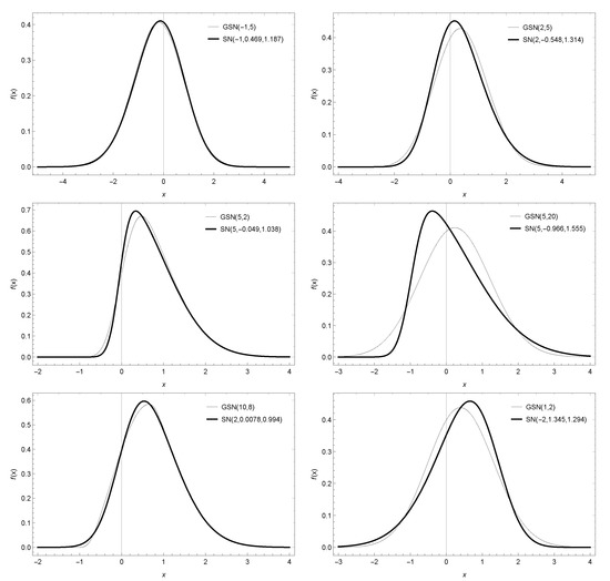
Figure 1.
Plot of the pdf (4) (thick line) denoted as GSN() and the SN() (thin line) for selected values of the parameters and .
Other possibilities for which we can get simple expressions for the corresponding pdf by applying (3) include the hyperbolic secant distributions (see [26,27], among others) and the ArcSin distributions (see [28]).
On some occasions, it is convenient expressed (3) as
which is obtained after the change of variable in (3). In fact the family of skew distributions given in [5] can alternatively be obtained from (5) by applying the first mean value Theorem to the integral appearing on (5) in the interval . To see this take in the well known formula , , to obtain .
2.2. The Second Family of Skew Distributions
Now we present the second family of skew distributions proposed in this work. This is derived from Equation (5) as follows.
Theorem 3.
If be a density function that is symmetric about zero and a cdf also symmetric about zero, then,
is a valid pdf for and .
Proof.
From Equation (3) it follows that
If we now take the derivative with respect to on both sides in (7) and apply the Fundamental Theorem of calculus we get
Thus Equation (6) is a genuine pdf. □
It can be verified that the pdf’s given in (6) also satisfy the properties listed in Proposition 1. Furthermore, it is straightforward to see that , and .
Note that the two proposed families, (3) and (6), are different and the only density belonging to both families is the basic density . A major difference between the two proposed families is that in the first family is not permitted to take the value zero while that is permitted in the second family. Both families are very similar and differ markedly only in small regions of the support of the distributions. To see this, note that applying the trapezoid rule to (3) we get
which coincides with (5).
Because , from (6) we get that when , while for we get the skew family of distributions proposed in Reference [5]. Again, it can be verified that for the family given in Equation (6). Thus the same identifiability problem arises for the model (6) as did in the model (3) if we allow to assume both positive and negative values. To avoid this problem here too we can and will restrict to be non-negative when discussing inference for the model. If desired, a more general class than the one proposed in (6) is one corresponding to finite mixtures of densities of the form (6) as follows
where the ’s are positve and
At this point, we give a more general result than the one provided in [5,29,30] for a symmetric random variable.
Proposition 2.
If U be a random variable that is symmetric about zero with cdf given by , pdf and if λ and α are two real numbers, then,
Proof.
This is obtained in a straightforward way directly from the result given in Theorem 3 by integrating on both sides of the equality over the support . □
When U follows a standard normal distribution (9) reduces to
a result which is well known in the statistical literature (see [5,29,30]).
3. The Normal Distribution Case
Of greater interest, because it is expressed in a simpler formulation, is the pdf obtained from Equation (6) when g and G are replaced by the pdf and cdf of the standard normal distribution, respectively. This is given by
In the folowing discussion, when a random variate X has its pdf given by Equation (10) it will be denoted by . Figure 2 show some graphs of this pdf and the corresponding skew normal pdf with the same mean and variance. (In this case, the skew parameter of the SN distribution has been set so that, once equal to the mean and variance of the new distribution, the values of and were obtained numerically so that both distributions should have the same mean and the same variance. It can be seen that the new model is very versatile and that the value of the parameters provide a distribution which can exhibit unimodality and bimodality. Again, as with Figure 1, the distribution can take approximately the same shape as the normal skew distribution with fewer parameter).
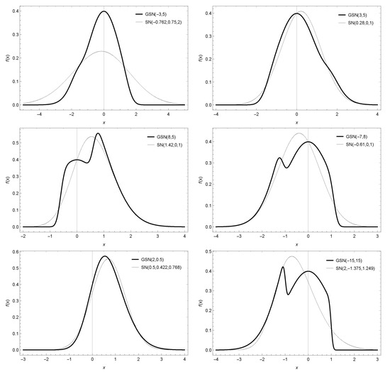
Figure 2.
Plot of the pdf in (10) for selected values of parameters and comparison with the skew normal one.
We next provide the moment generating function of the family given in Equation (10).
Proposition 3.
The moment generating function of a random variable X having its pdf given by Equation (10) is of the form
where
Proof.
It is straightforward following the same argument as the one used in Reference [5] in order to get the moment generating function of the skew-normal distribution. □
Moments can then be readily obtained by differentiation of Equation (11). In particular, the mean and variance are given by
where . Table 1 shows the mean and variance of the proposed distribution and the corresponding ones for the skew normal distribution for some special cases of parameters. Similar to case of the skew normal distribution, it can be verified that . Another important property that shares with the skew normal distribution is that if then for all values of and . In complete moments can also be studied following the work of Reference [31]. The third (skewness) and fourth (kurtosis) standardised cumulants are given by,
where
and and are given by Equations (12) and (13), respectively. Comparisons of these values with the standard skew normal distribution are shown in Table 2. As can be seen, the standardized fourth central moment (kurtosis) can be lower for the GSN distribution than it is for Azzalini’s skew normal distribution.

Table 1.
Mean and variance of the GSN and the SN variates for some parameter values.
Table 2.
Third and fourth standardized cumulants of the GSN and the SN variates for some parameter values.
Let denote the cdf of .
Proposition 4.
If , then its cdf is given by
where is the Owen’s function see [32] given by
Proof.
The proof is direct by applying result B.21 in Reference [21]. □
Proposition 5.
If , then it follows that:
- .
- .
- .
Proof.
The proof is also direct this time by applying the result B.23 in [21]. □
To end this Section we provide a result related to probability transformations which generalises a result appearing in Reference [5] and provided also in Reference [31].
Proposition 6.
Let W and Z be independent random variables with distribution and , respectively. The n, the random variable , where , follows a , where and .
Proof.
It can be proved following the same argument as that used in Lemma 1 in Reference [31]. □
4. Estimation
The family of distributions can be generalized by means of a linear transformation in order to introduce a location and a scale parameter adding more flexibility to the model (10). We thus will consider the location-scale generalization of the skew-normal distribution defined as the distribution of , where given in Equation (10), where and . Its pdf is given by
When this pdf reduces to the and when to the . For a sample we can estimate the four parameters, , of the model given in Equation (14) by a direct search for the maximum of the log-likelihood surface given by
Since it is not possible to obtain closed expressions for the maximum likelihood estimators, algorithms based on numerical methods, such as Newton-Raphson or Broyden-Fletcher-Goldfarb-Sanno (BGGS), among others, will have to be used. It is recommended to use different seed points as initial values to ensure that the solution obtained constitutes a global maximum of the logarithm-likelihood function.
The standard errors of the estimators can be obtained by inverting the Hessian matrix. Both Mathematica and WinRats have at least two methods for this purpose. The first is to use Cholesky factors (this package is available on the web upon request). The second, faster method, involves by finite differentiation. Furthermore, WinRats package also offers the possibility to get the maximum of the log-likelihood directly giving us the elements of the Fisher information matrix. In fact, for the examples considered later these two packages were used to get the maximum likelihood estimators in a fast way.
5. Multivariate Versions
Multivariate extensions of the univariate distributions arise in an easy way as we can see in the next result.
Theorem 4.
Let X and be two random variables where and . The n,
represents a genuine pdf for and .
Proof.
Without loss of generality, asume that X and are independent random variables. Taking into account the fact that is symmetric and using the result provided in Theorem 1, we get
Hence the result. □
Remark 1.
The only important required property of the distribution of is that, for any , the random variable is symmetric about zero. The only required property for the distribution of X is that it be symmetric about zero. This is true for the above Theorem and the next.
Theorem 5.
Let X and be two random variables where and . The n,
is a valid pdf for and .
Proof.
From (16) it follows that
If we now take the derivative with respect to on both sides in Equation (18) and apply the Fundamental Theorem of calculus we get
Thus (17) is a genuine pdf. □
Note that if we set in (17), we obtain
which was one of the first multivariate skew-normal models to appear in the literature. See [10,11], for instance.
Figure 3 shows the density for bivariate generalized skew-normal (BGSN) model for some combinations of the parameters. Perusal of Figure 3, will confirm that the density of the BGSN model exhibits a more interesting array of possible shapes than do many of its competitors. The flexibility of this model can be expected to be useful in fitting the model to a variety of different data sets.
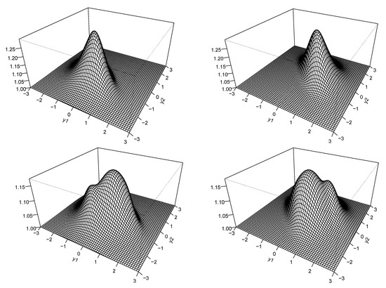
Figure 3.
Density for BGSN for: and (upper left panel); and (upper right panel); and (lower left panel); and (lower right panel).
6. Numerical Illustrations
In this section, three examples for the GSN model given in Equation (14) are carried out and the results are compared with the flexible epsilon skew-normal (FESN) model introduced by Reference [33] in the first example, with the mixture of two normals (MN) model in the second example and flexible skew-normal (FSN) model introduced by Reference [34] in the third example. The three densities respectively are given by:
where and denote the density and distribution functions of the standard normal distribution, , , , and .
We use these three models, since they have been used in the applied statistics literature to explain bimodal empirical data. We chose the MN model since it is a classic model that is used to model bimodal data sets, we chose the FESN model since it is one of the first bimodal extensions of the family of epsilon-skew-simétric distributions and We chose the FSN model since it is one of the first bimodal extensions of the family of skew-simétric distributions.
6.1. Example 1
The data in this example is a set of fiber levels for 315 patients and is available online at http://Lib.stat.cmu.edu/datasets/Plasma_Retinol and contains values for 14 variables for each patient. For our analysis we will use only the variable called Fiber (Grams of fiber consumed per day). Low levels of this variable may be associated with higher risk of certain types of cancer. Descriptive statistics for the data set are displayed in Table 3. In the table and denote sample skewness and kurtosis coefficients. Note that the data exhibits a high level of kurtosis.
Table 3.
Fiber: Descriptive statistics.
The estimated values of the parameters for the two models are shown in Table 4 together with the standard errors (SE) in parentheses. The table also includes the maximum of the log-likelihood function (), the Akaike information criterion (AIC) and the consistent Akaike information criterion (CAIC), proposed in References [35,36] respectively. Amodel with a lower AIC or CAIC is preferred to a model with a higher value.
Table 4.
Parameter estimates (SE) for FESN and GSN models.
Graphs of histogram of the data and fitted densities are given in Figure 4. As it can be seen, the GSN distribution is the better of the two models with regard to reflecting the nature of the empirical data. All computations here were done using Mathematica v.11.0 and WinRATS v.7.0. These codes are available from the authors upon request.
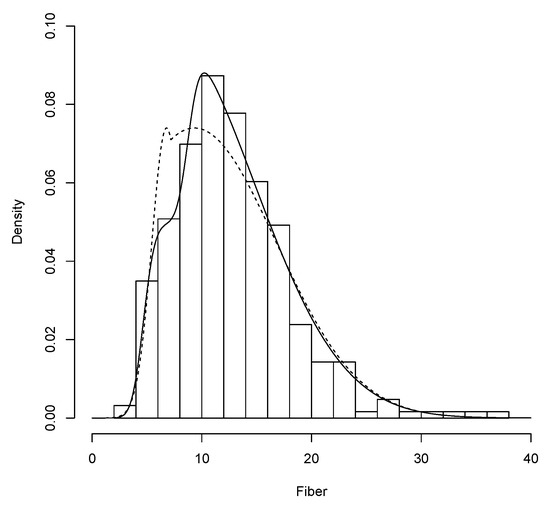
Figure 4.
FESN distribution (dashed line) and GSN distribution (solid line) for the Fiber data.
6.2. Example 2
We consider the variables M-Sweet available in the database creaminess of cream cheese which can be found at http://www.models.kvl.dk/research/data/Cream/index.asp.
Table 5 shows summary statistics for the M-Sweet dataset.
Table 5.
M-Sweet: Descriptive statistics.
In Table 6, presents parameter estimates (SE) for both, the MN and GSN models. It can be seen that the log-likelihood for the GSN model is higher than the for the MN model. The AIC and CAIC criterion are used again to compare the estimated models, it can be seen that the GSN model presents the best fit (smallest AIC and CAIC values).
Table 6.
Parameter estimates (SE) for MN and GSN models.
Finally, the histogram of the data and the fitted densities are shown in Figure 5.
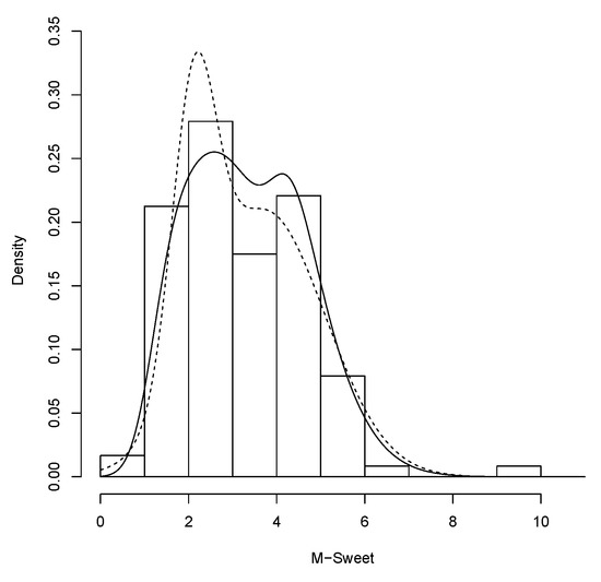
Figure 5.
MN distribution (dashed line) and GSN distribution (solid line) for the M-Sweet data.
6.3. Example 3
Finally, data corresponding to the age and frequency of cancer cataloged as Kaposi’s sarcoma have been taken. This is a type of cancer that can form masses in the skin, lymph nodes, or other organs without distinguishing the sub-types. The data has been collected from the website of the Office for National Statistics (ONS, section Health statistics) and it can be seen in Table A1 in the Appendix A. It can be observed that there is a higher incidence in individuals with an age around 25 years as well as for those with an age around 60 years. The se records were taken during the years 1995–2016 and correspond to different regions of the United Kingdom. Table 7 shows summary statistics for the Kaposi’s sarcoma dataset.
Table 7.
Kaposi’s sarcoma: Descriptive statistics.
The two fitted models are represented in Figure 6 and the correspondent estimated values can be seen in Table 8. The GSN model presents better fit for the data, since the AIC and CAIC values are smaller.
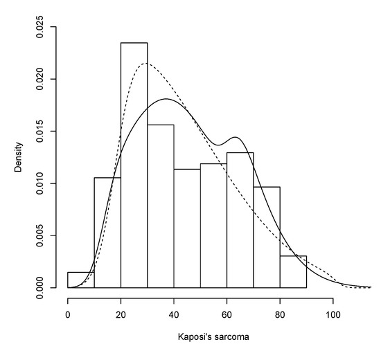
Figure 6.
FSN distribution (dashed line) and GSN distribution (solid line) for the Kaposi’s sarcoma data.
Table 8.
Parameter estimates (SE) for FSN and GSN models.
7. Conclusions
We have proposed two families of skew distributions which can be considered as alternatives to the well-known skew normal distribution for fitting skewed data.
Future research could address the following issue. We can ask whether the methodology proposed here can be applied to the generalized skew-normal distribution proposed by Reference [9] to obtain a more flexible distribution. For the case with standard normal components, one might consider the following model which is an average of two Arnold and Beaver densities.
where . Note that this model is not obtainable by methods analogous to those used to develop the model (10). However, it is a simple more flexible extension of the Arnold-Beaver model. But, once we recognize it as a mixture with equal weights, it is resonable to add more flexibility by considering unequal weights, as follows
where
Author Contributions
Conceptualization, E.G.-D., B.C.A. and J.M.S.; Formal analysis, E.G.-D., B.C.A., J.M.S. and H.W.G.; Investigation, E.G.-D., B.C.A., J.M.S. and H.W.G.; Methodology, E.G.-D. and J.M.S.; Software, E.G.-D. and H.W.G.; Supervision, E.G.-D. and B.C.A.; Validation, E.G.-D. and H.W.G. All of the authors contributed significantly to this research article. All authors have read and agreed to the published version of the manuscript.
Funding
The authors thank to the Ministerio de Economía y Competitividad, Spain (project ECO2017-85577-P, EGD and Ministerio de Ciencia e Innovación, Spain (PID2019-105986GB-C22), JMS for partial support of this work. The research of H.W. Gómez was supported by PUENTE-UA project, Chile.
Acknowledgments
The authors thank the Editor and three anonymous referees for their constructive comments and suggestions, which have greatly helped them to improve the paper.
Conflicts of Interest
The authors declare no conflict of interest.
Appendix A
Table A1.
Data corresponding to Kaposi’s sarcoma.
Table A1.
Data corresponding to Kaposi’s sarcoma.
| Age | Number |
|---|---|
| 1 | 1 |
| 5 | 89 |
| 10 | 342 |
| 15 | 718 |
| 20 | 2352 |
| 25 | 3593 |
| 30 | 3243 |
| 35 | 2533 |
| 40 | 2015 |
| 45 | 1747 |
| 50 | 1562 |
| 55 | 1662 |
| 60 | 1801 |
| 65 | 1915 |
| 70 | 1855 |
| 75 | 1611 |
| 80 | 1203 |
| 85 | 642 |
| 90 | 247 |
References
- Aigner, D.J.; Lovell, C.A.K.; Schmidt, P. Formulation and estimation of stochastic frontier production functions. J. Econ. 1977, 6, 21–37. [Google Scholar] [CrossRef]
- Kumbhakar, S.C.; Parmeter, C.F.; Tsionas, E.G. A zero inefficiency stochastic frontier model. J. Econ. 2013, 172, 66–76. [Google Scholar] [CrossRef]
- Marshall, A.W.; Olkin, I. A new method for adding a parameter to a family of distributions with application to the exponential and Weibull families. Biometrika 1997, 84, 641–652. [Google Scholar] [CrossRef]
- Jones, M.C. Families of distributions arising from distributions of order statistics. Test 2007, 13, 1–43. [Google Scholar] [CrossRef]
- Azzalini, A. A class of distributions which includes the normal ones. Scan. J. Stat. 1985, 12, 171–178. [Google Scholar]
- Henze, N. A probabilistic representation of the Skew-Normal distribution. Scan. J. Stat. 1986, 4, 271–275. [Google Scholar]
- Silver, E.A.; Costa, D. A property of symmetric distributions and a related order statistic result. Am. Stat. 1997, 51, 32–33. [Google Scholar]
- Gupta, R.C.; Gupta, R.D. Generalized skew normal model. Test 2004, 12, 501–524. [Google Scholar] [CrossRef]
- Arnold, B.C.; Beaver, R.J. Skewed multivariate models related to hidden truncation and/or selective reporting (with discussion). Test 2002, 11, 1–54. [Google Scholar] [CrossRef]
- Azzalini, A.; Capitanio, A. Statistical applications of the multivariate skew-normal distribution. J. R. Stat. Soc. Ser. B 1999, 61, 579–602. [Google Scholar] [CrossRef]
- Azzalini, A.; Valle, A. The multivariate skew-normal distribution. Biometrika 1996, 83, 715–726. [Google Scholar] [CrossRef]
- Azzalini, A. Further results on a class of distributions which includes the normal ones. Statistica 1986, 46, 199–208. [Google Scholar]
- Azzalini, A.; Chiogna, M. Some results on the stress-strength model for skew-normal variates. METRON 2004, LXII, 315–326. [Google Scholar]
- Gupta, R.D.; Gupta, R.C. Analyzing skewed data by power normal model. Test 2008, 17, 197–210. [Google Scholar] [CrossRef]
- Gómez, H.; Venegas, O.; Bolfarine, H. Skew-symmetric distributions generated by the distribution function of the normal distribution. Environmetrics 2007, 18, 395–407. [Google Scholar] [CrossRef]
- Sharafi, M.; Behboodian, J. The Balakrishnan skew-normal density. Stat. Paper. 2008, 49, 769–778. [Google Scholar] [CrossRef]
- Jones, M.; Pewsey, A. Sinh-arcsinh distributions. Biometrika 2009, 96, 761–780. [Google Scholar] [CrossRef]
- Gómez-Déniz, E.; Iriarte, Y.A.; Calderín-Ojeda, E.; Gómez, H.W. Modified Power-Symmetric Distribution. Symmetry 2019, 11, 1410. [Google Scholar] [CrossRef]
- Alavi, S.M.R.; Tarhani, M. On a Skew Bimodal Normal-Normal distribution fitted to the Old-Faithful geyser data. Commun. Stat. Theor. Method. 2017, 46, 7301–7312. [Google Scholar] [CrossRef]
- García, V.; Gómez-Déniz, E.; Vázquez-Polo, F. A new skew generalization of the normal distribution: Properties and applications. Comput. Stat. Data Anal. 2010, 54, 2021–2034. [Google Scholar] [CrossRef]
- Azzalini, A. The Skew Normal and Related Families; Cambridge University Press: Cambridge, UK, 2014. [Google Scholar]
- Dickson, D. InSurance Risk and Ruin; Cambridge University Press: Cambridge, UK, 2005. [Google Scholar]
- Rolski, T.; Schmidli, H.; Schmidt, V.; Teugel, J. Stochastic Processes for Insurance and Finance; John Wiley and Sons: Hoboken, NJ, USA, 1999. [Google Scholar]
- Burdick, D. A note on symmetric random variables. Annal. Math. Stat. 1972, 43, 2039–2040. [Google Scholar] [CrossRef]
- Jones, M. Generating distributions by transformation of scale. Stat. Sinica 2014, 24, 749–771. [Google Scholar] [CrossRef][Green Version]
- Ding, P. Three Occurrences of the Hyperbolic-Secant Distribution. Am. Stat. 2014, 68, 32–35. [Google Scholar] [CrossRef]
- Johnson, N.; Kotz, S.; Balakrishnan, N. Continuous Univariate Distributions; Wiley: New York, NY, USA, 1995. [Google Scholar]
- Arnold, B.C.; Groeneveld, R.A. Some Properties of the Arcsine Distribution. J. Am. Stat. Assoc. 1980, 75, 173–175. [Google Scholar] [CrossRef]
- Ellison, B. Two theorems for inferences about the normal distribution with applications in acceptance sampling. J. Am. Stat. Assoc. 1964, 59, 89–95. [Google Scholar] [CrossRef]
- Zacks, S. Parametric Statistical Inference; Pergamon Press: Oxford, UK, 1981. [Google Scholar]
- Chiogna, M. Some results on the scalar skew-normal distribution. J. Ital. Statist. Soc. 1998, 1, 1–13. [Google Scholar] [CrossRef]
- Owen, D. Tables for computing bivariate normal probabilities. Ann. Math. Stat. 1956, 27, 1075–1090. [Google Scholar] [CrossRef]
- Arellano-Valle, R.B.; Cortés, M.A.; Gómez, H.W. An Extension of the Epsilon-Skew-Normal Distribution. Communicat. Stat. Theor. Method. 2010, 39, 912–922. [Google Scholar] [CrossRef]
- Yanyuan, M.A.; Genton, M.G. Flexible Class of Skew-Symmetric Distributions. Scand. J. Stat. 2004, 31, 459–468. [Google Scholar]
- Bozdogan, H. The general theory and its analytical extension. Psychometrika 1987, 52, 345–370. [Google Scholar] [CrossRef]
- Akaike, H. A new look at the statistical model. IEEE Transact. Automat. Control. 1974, 19, 716–723. [Google Scholar] [CrossRef]
Publisher’s Note: MDPI stays neutral with regard to jurisdictional claims in published maps and institutional affiliations. |
© 2021 by the authors. Licensee MDPI, Basel, Switzerland. This article is an open access article distributed under the terms and conditions of the Creative Commons Attribution (CC BY) license (http://creativecommons.org/licenses/by/4.0/).