On the Numerical Simulation of HPDEs Using θ-Weighted Scheme and the Galerkin Method

Abstract

Herein, an efficient algorithm is proposed to solve a one-dimensional hyperbolic partial differential equation. To reach an approximate solution, we employ the $\theta$-weighted scheme to discretize the time interval into a finite number of time steps. In each step, we have a linear ordinary differential equation. Applying the Galerkin method based on interpolating scaling functions, we can solve this ODE. Therefore, in each time step, the solution can be found as a continuous function. Stability, consistency, and convergence of the proposed method are investigated. Several numerical examples are devoted to show the accuracy and efficiency of the method and guarantee the validity of the stability, consistency, and convergence analysis.

1. Introduction

Partial differential equations (PDEs) are ubiquitous in mathematically scientific fields and play an important role in engineering and physics. They arise from many purely mathematical considerations, such as the calculus of variations and differential geometry. One of the momentous subclasses of PDEs is the hyperbolic partial differential equations (HPDEs). HPDEs are used to model many phenomena such as biology, industry, atomic physics, and aerospace [1,2,3]. Telegraph and wave equations are the most famous types of HPDEs that are enforceable in various fields such as random walk theory, wave propagation, and signal analysis [2,4].

In this study, we construct and analyze a numerical algorithm based on the $\theta$-weighted method, and the Galerkin method to solve the HPDEs

$$w_t(x,t)+a_1{w}_x(x,t)+a_{2}w(x,t)=f(x,t),x\in [0,1],t\in [0,T],$$

(1)

with boundary condition

$$w(0,t)=g\left(t\right),t\in [0,T],$$

(2)

and initial condition

$$w(x,0)=h\left(t\right),x\in [0,1].$$

(3)

Furthermore, we assume that f, g, and h are the known functions, and also $a_1$ and $a_2$ are real constants.

In this paper, we attempt to apply an efficient scheme that has not been used before to solve such problems. The method includes three steps. In the first step, we use the $\theta$-weighted method to break the time interval into a finite number of time steps. At each time step, we obtain a linear ordinary differential equation. In the second step, the obtained ODE is solved using the Galerkin method. To do this, interpolating scaling functions are used. In comparison to the scaling function arising from multiresolution analysis (MRA), interpolation scaling functions (ISFs) have some properties that make them attractive. These characteristics include the flexible zero moments, a compact support, orthonormality, and having a closed-form. The most important property of these bases is the interpolation. This property is useful to avoid integrals to find coefficients in expansions. At the last step, the linear algebraic system obtained from the second one must be solved using an appropriate technique. Stability, consistency, and convergence analysis are investigated, and numerical tests guarantee their validity.

Numerous studies proposed a variety of numerical and analytical solutions to HPDEs. Doha et al. [5] proposed a numerical method based on the collocation method for solving a system consisting of such equations. In [6], the spectral-Galerkin method is proposed to solve this equation. Singh et al. [7] solved one-dimensional HPDEs with the initial and boundary conditions (2) and (3), using an algorithm based on Chebyshev and Legendre multiwavelets. Dehghan et al. [8] introduced a numerical scheme based on the cubic B-spline scaling functions to solve (1) with nonlocal conservation conditions. Bin Jebreen et al. [4] proposed an efficient method based on the wavelet Galerkin method to solve the Telegraph equation, and the collocation method based on interpolating scaling functions is also used for solving this equation in [3]. For study, we refer the readers to [9,10].

The outline of the paper is as follows. Section 2 is devoted to the brief introduction to the interpolating scaling function. Mixed $\theta$-weighted scheme and Galerkin method based on interpolating scaling functions are used to solve the desired equation and the stability, consistency, and convergence analysis are also investigated in Section 3. Section 4 is devoted to some numerical examples to show the ability and accuracy of the proposed method.

2. Interpolating Scaling Functions

To derive a set of bases that covers the multiresolution analysis conditions, Alpert et al. [11] introduced a set of functions to generate the nested spaces ${\left\{V_J^r\right\}}_{J=0}^{\infty }\in L_2\left([0,1]\right)$ using piecewise polynomial bases of degree less than $r\ge 0$ (the multiplicity parameter). Let $J\in {\mathbb{Z}}^{+}\cup \left\{0\right\}$ be given. Putting ${\mathcal{B}}_J:=\{0,\dots ,2^J-1\}$, and $\mathcal{R}:=\{0,1,\cdots ,r-1\}$, there is a sequence of nested subspaces that are spanned by

$$V_J^r:=Span\{{\varphi }_{J,b}^k:={\varphi }^k(2^{J}x-k),b\in {\mathcal{B}}_J,k\in \mathcal{R}\}\subset L_2\left([0,1]\right),r\ge 0,J\in {\mathbb{Z}}^{+}\cup \left\{0\right\},$$

by means of the Interpolating scaling functions ${\left\{{\varphi }^k\right\}}_{k\in \mathcal{R}}$, introduced by Alpert using the Legendre polynomials. Assume that $P_r$ is the Legendre polynomial of order r and ${\left\{{\tau }_k\right\}}_{k\in \mathcal{R}}$ are the roots of $P_r$. Let ${\left\{{\omega }_k\right\}}_{k\in \mathcal{R}}$ be the Gauss–Legendre quadrature weights [3,11]. We determine ISFs as follows:

$${\varphi }^k\left(x\right)=\left\{\begin{array}{cc}\sqrt{\frac{2}{{\omega }_k}}{L}_k(2x-1),& x\in [0,1],\hfill \\ 0,& o.w,\hfill \end{array}\right.$$

where ${\left\{L_k\left(x\right)\right\}}_{k\in \mathcal{R}}$ are the Lagrange polynomials

$$L_k\left(x\right)=\prod _{i=0,i\ne k}^{r-1}\left(\frac{x-{\tau }_i}{{\tau }_k-{\tau }_i}\right).$$

These bases fulfill the orthonormality relation $\langle {\varphi }_{J,b}^k,{\varphi }_{J,b^{\prime }}^{k^{\prime }}\rangle ={\delta }_{b,b^{\prime }}{\delta }_{k,k^{\prime }}$ where $\langle .,.\rangle$ denotes the $L_2$-inner product on $\Omega :=[0,1]$.

Assume that ${\cup }_{b\in \mathcal{B}}{I}_{J,b}$ is a uniform finite discretization of $\Omega$. Here, the subintervals $I_{J,b}:=[x_b,x_{b+1}]$ are specified by points $x_b:=b/\left(2^J\right)$. To project a function into $V_J^r$, we introduce the orthogonal projection ${\mathcal{P}}_J^r$ that maps $L^2(\Omega )$ onto the subspace $V_J^r$. Utilizing this projection, every function $p\in L_2(\Omega )$ can be represented in the form

$$p\approx {\mathcal{P}}_J^r\left(p\right)=\sum _{b\in {\mathcal{B}}_J}\sum _{k\in \mathcal{R}}{p}_{J,b}^k{\varphi }_{J,b}^k.$$

(4)

Due to the orthonormality of the bases, it is easy to prove that the coefficients $p_{J,b}^k$ can be obtained by $\langle p,{\varphi }_{J,b}^k\rangle ={\int }_{I_{J,b}}p\left(x\right){\varphi }_{J,b}^k\left(x\right)dx$. To avoid integration, we apply the interpolation property of ISFs [11,12], via

$$p_{J,b}^k\approx 2^{-J/2}\sqrt{\frac{{\omega }_k}{2}}p\left(2^{-J}(\frac{{\tau }_k+1}{2}+b)\right),b\in {\mathcal{B}}_J,k\in \mathcal{R}.$$

(5)

Given r-times continuously differentiable function $p\in C^r(\Omega )$, the projection ${\mathcal{P}}_J^r\left(p\right)$ is bounded by means of $L_2$-inner product as

$$\parallel {\mathcal{P}}_J^r\left(p\right)-p\parallel \le 2^{-Jr}\frac{2}{4^{r}r!}\underset{x\in [0,1]}{sup}\left|p^{\left(r\right)}\left(x\right)\right|.$$

(6)

According to this relation, the projection ${\mathcal{P}}_J^r$ is convergent when J or r increases. To study more details, we refer the readers to [13]. Consequently, this projection is convergent with the rate of $O\left(2^{-Jr}\right)$.

We determine the vector function ${\Phi }_J^r:={[{\Phi }_{r,J,0},\cdots ,{\Phi }_{r,J,2^J-1}]}^T$ with ${\Phi }_{r,J,b}:=[{\varphi }_{J,b}^0,\cdots ,{\varphi }_{J,b}^{r-1}]$ includes the scaling functions and called multi-scaling functions. The approximation (4) can be rewritten using the vector P whose entries are $P_{br+k+1}:=p_{J,b}^k$ as follows:

$${\mathcal{P}}_J^r\left(p\right)=P^T{\Phi }_J^r,$$

(7)

where P is a vector of dimensional $N:=r{2}^J$.

To approximate a higher-dimensional function, the building blocks of the bases can be utilized. In this regard, one can consider the subspace $V_J^{r,2}:=V_J^r\times V_J^r\subset L^2(\Omega \times \Omega )$ that is spanned by

$$\{{\varphi }_{J,b}^k{\varphi }_{J,b^{\prime }}^{k^{\prime }}:b,b^{\prime }\in {\mathcal{B}}_J,k,k^{\prime }\in \mathcal{R}\}.$$

In order to derive an approximation of two-dimensional function $p\in L^2(\Omega \times \Omega )$, we apply the projection operator ${\mathcal{P}}_J^r$, viz.

$$p(x,t)\approx {\mathcal{P}}_J^r\left(p\right)(x,t)={{\Phi }_J^r}^T\left(x\right)P{\Phi }_J^r\left(t\right),$$

(8)

where components of the square matrix P of order N are obtained by

$$P_{rb+(k+1),r{b}^{\prime }+(k^{\prime }+1)}\approx 2^{-J}\sqrt{\frac{{\omega }_{k^{\prime }}}{2}}\sqrt{\frac{{\omega }_k}{2}}p\left(2^{-J}({\widehat{\tau }}_k+b),2^{-J}({\widehat{\tau }}_{k^{\prime }}+b^{\prime })\right),$$

(9)

and ${\widehat{\tau }}_k=({\tau }_k+1)/2$. If $C^{\left(2r\right)}(\Omega \times \Omega )\ni p:\Omega \times \Omega \to \mathbb{R}$, we can show that the error can be bounded as follows:

$$\parallel {\mathcal{P}}_J^{r}p-p\parallel \le {\mathcal{M}}_{max}\frac{2^{1-rJ}}{4^{r}r!}\left(2+\frac{2^{1-Jr}}{4^{r}r!}\right),$$

(10)

where ${\mathcal{M}}_{max}$ is a constant [12] as follows:

$${\mathcal{M}}_{max}=max\left\{\underset{\xi \in [0,1)}{sup}|\frac{{\partial }^r}{\partial x^r}p(\xi ,t)|,\underset{\eta \in [0,1)}{sup}|\frac{{\partial }^r}{\partial t^r}p(x,\eta )|,\underset{{\xi }^{\prime },{\eta }^{\prime }\in [0,1)}{sup}|\frac{{\partial }^{2r}}{\partial x^r\partial t^r}p({\xi }^{\prime },{\eta }^{\prime })|\right\}.$$

3. Numerical Method of Solution

The main idea behind the proposed method is based on the $\theta$-weighted scheme and Galerkin methods. In the first step, the $\theta$-weighted method is used to discretize the time interval into a finite number of time steps. The linear system of ordinary differential equations obtained after the first step can be reduced to a system of algebraic equations by using the Galerkin method in the second one. Thus, one can find the approximate solution of the desired equation at the time step points $t_n:=n\delta t$, $n=0,\dots ,M$ ($t_n\in [0,T]$ and $T=M\delta t$).

To discretize the time variable, we use the $\theta$-weighted scheme as follows:

$$\frac{w^{n+1}-w^n}{\delta t}+\theta \left(a_1{w}_x^{n+1}+a_2{w}^{n+1}\right)+(1-\theta )\left(a_1{w}_x^n+a_2{w}^n\right)=f(x,t^n)+\mathfrak{R},$$

(11)

where for simplicity $w(x,t^n)$ is assumed to be $w^n$, for $t^n=t^{n-1}+\delta t$ (or equivalently $t^n=n\delta t$), and also $\mathfrak{R}\le \mathfrak{C}\delta t$ for a positive constant $\mathfrak{C}$ and $\theta \in [0,1]$ is a constant. Note that, by selecting the different values for $\theta$, one can find various methods, such as implicit method ($\theta =1$), explicit method ($\theta =0$), and the Crank–Nicolson method ($\theta =1/2$).

Since the remainder term $\mathfrak{R}$ is a small quantity, one can neglect it and, after simplification, we obtain

$$w^{n+1}+\theta \delta t\left(a_1{w}_x^{n+1}+a_2{w}^{n+1}\right)=w^n-(1-\theta )\delta t\left(a_1{w}_x^n+a_2{w}^n\right)+\delta tf(x,t^n),n=0,\dots ,M.$$

(12)

Next, this system of ordinary differential equations would be discretized by the Galerkin method based on ISFs. To this end, one can approximate the solution $w^n$ of (12) using the projection operator ${\mathcal{P}}_J^r$, via

$$w^n\left(x\right)\approx {\mathcal{P}}_J^r\left(w^n\right)\left(x\right)={W_n}^T{\Phi }_J^r\left(x\right),n=0,\dots ,M,$$

(13)

where $W_n$, for $n=1,\dots ,M$ is a vector of dimension N which must be found. The same approximation could be imagined to $w_x^n$, as

$$w_x^n\left(x\right)\approx {\mathcal{P}}_J^r\left(w_x^n\right)\left(x\right)={W_n}^T{D}_{\varphi }{\Phi }_J^r\left(x\right),n=0,\dots ,M,$$

(14)

where $D_{\varphi }$ is the operational matrix for derivative introduced in [14,15,16].

Replacing (13) and (14) in (12) yields

$$\left({W_{n+1}}^T+\theta \delta t\left(a_1{W_{n+1}}^T{D}_{\varphi }+a_2{W_{n+1}}^T\right)\right){\Phi }_J^r\left(x\right)=\left({W_n}^T-(1-\theta )\delta t\left(a_1{W_n}^T{D}_{\varphi }+a_2{W_n}^T\right)+\delta t{F}_n^T\right){\Phi }_J^r\left(x\right),$$

(15)

where $F_n$ is a $N\times 1$ vector that is obtained by projecting the function $f^n$ into $V_J^r$, viz.

$$f^n\approx {\mathcal{P}}_J^r\left(f^n\right)\left(x\right)=F_n^T{\Phi }_J^r\left(x\right),n=0,\dots ,M.$$

Let

$$\begin{array}{cc}\hfill A^T& :=(1+a_2\theta \delta t)I+a_1\theta \delta t{D}_{\varphi },\hfill \\ \hfill b^T& :=W_n^T\left((1-a_2(1-\theta )\delta t)I-a_1(1-\theta )\delta t{D}_{\varphi }\right)+\delta t{F}_n^T,n=0,\dots ,M,\hfill \end{array}$$

(16)

where I is the identity matrix of dimension N. Multi-scaling function ${\Phi }_J^r\left(x\right)$ are orthonormal bases for $V_J^r$. Thus, they are linearly independent, and then we have the following linear system:

$$A{W}_{n+1}=b.$$

(17)

To apply the boundary condition (2), it can also be projected into $V_J^r$, via

$$w^{n+1}\left(0\right)\approx W_{n+1}^T{\Phi }_J^r\left(0\right)=g\left(t^{n+1}\right).$$

(18)

Substituting the first row of A and the first element of b by ${{\Phi }_J^r\left(0\right)}^T$ and $g\left(t^{n+1}\right)$, respectively, we obtain the modified system

$$\tilde{A}{W}_{n+1}=\tilde{b}.$$

(19)

Now, note that, to start the steps, the initial condition should be utilized via

$$w(x,0)\approx W_0^T{\Phi }_J^r\left(x\right)=H^T{\Phi }_J^r\left(x\right),$$

(20)

and then $W_0=H$ where H is a vector of dimension N. Utilizing $W_0=H$, Equation (19) gives a system of equations at every time step $t^n$, $n=0,\dots ,M$. Thus, one can obtain the approximate solution $w(x,t^n)$ by means of a linear expansion of interpolating scaling function (13).

3.1. Stability

To analyze the stability of the time discretization by $\theta$-weighted scheme, assume that ${\widehat{w}}_{n+1}$ is the approximate solution of (17). We set $e^{n+1}:=w^{n+1}-{\widehat{w}}^{n+1}$ as the error that arises from the proposed Galerkin method. Consequently, the roundoff error satisfies

$$(1+a_2\theta \delta t)e^{n+1}+a_1\theta \delta t{e}_x^{n+1}=(1-a_2(1-\theta )\delta t)e^n-a_1(1-\theta )\delta t{e}_x^n.$$

(21)

Projecting the error $e^n$ using ${\mathcal{P}}_J^r$ into $V_J^r$, one can write

$$e^n\approx {\mathcal{P}}_J^r\left(e^n\right)=E_n^T{\Phi }_J^r.$$

(22)

Inserting (22) into (21) and applying the operational matrix of derivative for ISFs, we get

$${{\Phi }_J^r}^{T}A{E}_{n+1}={{\Phi }_J^r}^{T}B{E}_n,$$

(23)

where $B^T:=(1-a_2(1-\theta )\delta t)I-a_1(1-\theta )\delta t{D}_{\varphi }$. Provided the matrix A is inverted, it can be shown that

$$E_{n+1}=A^{-1}B{E}_n.$$

(24)

Taking the norm of both sides of (24), and using the matrix norm property, we obtain the following inequality:

$$\parallel E_{n+1}\parallel \le \parallel A^{-1}B\parallel \parallel E_n\parallel ,n=0,\dots ,M.$$

(25)

This gives rise to a sufficient and necessary condition for the stability of the method so that, in order to have a stable method, the spectral radius of the matrix $A^{-1}B$ must be less than one ($\rho <1$, where $\rho$ is a spectral radius of $A^{-1}B$).

3.2. Convergence Analysis

Assume that $e^{n+1}:=w^{n+1}-{\widehat{w}}^{n+1}$. Subtracting (12) from (15) and using the notations in the previous section, one can write after some simplification

$$\parallel E_{n+1}\parallel \le \parallel A^{-1}\parallel \parallel B\parallel \parallel E_n\parallel +\parallel A^{-1}\parallel \parallel f^n-{\widehat{f}}^n\parallel ,$$

(26)

where $f^n:=f(x,t^n)$ and ${\widehat{f}}^n:={\mathcal{P}}_J^r\left(f^n\right)$. Due to invertibility of matrix $D_{\varphi }$[11], it is obvious that $C_1:=\parallel A^{-1}\parallel$ and $C_2:=\parallel B\parallel$ are finite. Therefore, we have

$$\parallel E_{n+1}\parallel \le C_1\left(C_2\parallel E_n\parallel +\parallel f^n-{\widehat{f}}^n\parallel \right).$$

It follows from (6) that $\parallel E_n\parallel$ and $\parallel f^n-{\widehat{f}}^n\parallel$ are bounded

$$\parallel e^{n+1}\parallel \le C_1\frac{2^{1-Jr}}{4^{r}r!}(C_2\underset{x\in [0,1]}{sup}|{w^n}^{\left(r\right)}\left(x\right)|+\underset{x\in [0,1]}{sup}|{f^n}^{\left(r\right)}\left(x\right)|).$$

(27)

Note that $\theta$ plays an important role in the structure of $A^{-1}$ and B. Thus, the value of the variables $C_1$ and $C_2$ will change when the value of $\theta$ changes. These variables play a direct role in the error presented in (27).

We know that a method is consistent if, by reducing the mesh (by increase the refinement level J) and time step size ($\delta t$), the truncation error terms could be made to approach zero. Consequently, the inequality (27) confirms that the method is consistent at every time step when the refinement level J or multiplicity r increases.

If the condition for stability holds ($\rho \left(A^{-1}B\right)<1$) and if, for the Galerkin method, used for solving the ordinary differential equation at each time, the overall error approaches zero as $J\to \infty$ (indeed, the method is consistent), we usually find that the solution converges to the exact solution. This derives from the Lax Equivalence Theorem [17].

4. Numerical Results

To illustrate the validity of stability, consistency, and convergence analysis, some numerical tests have been considered in this section.

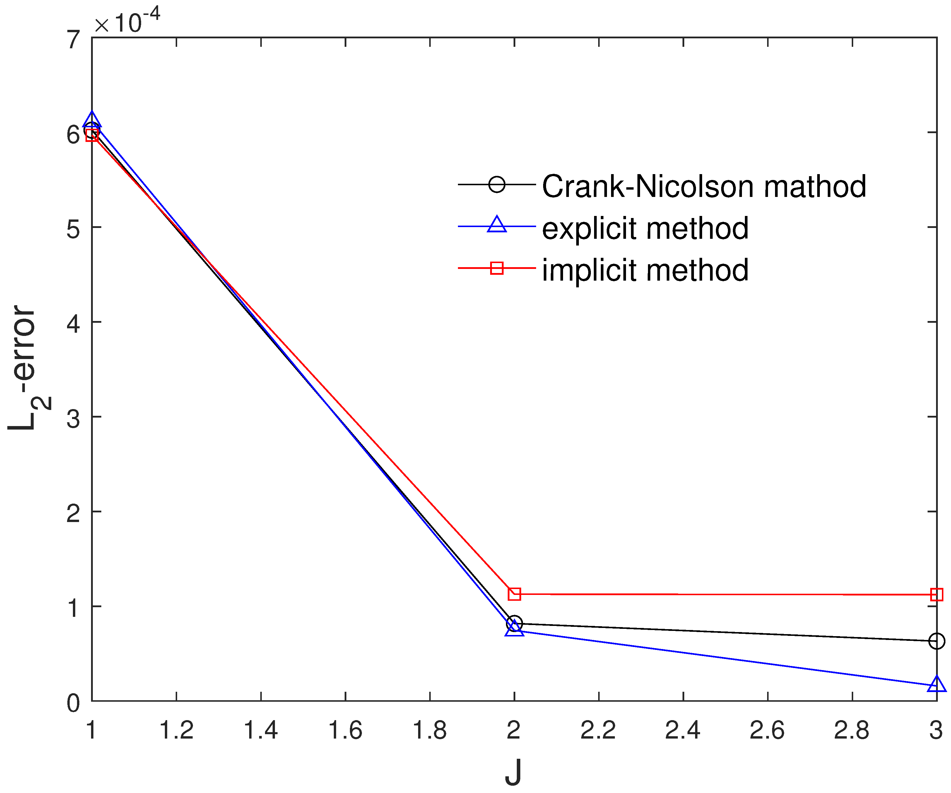
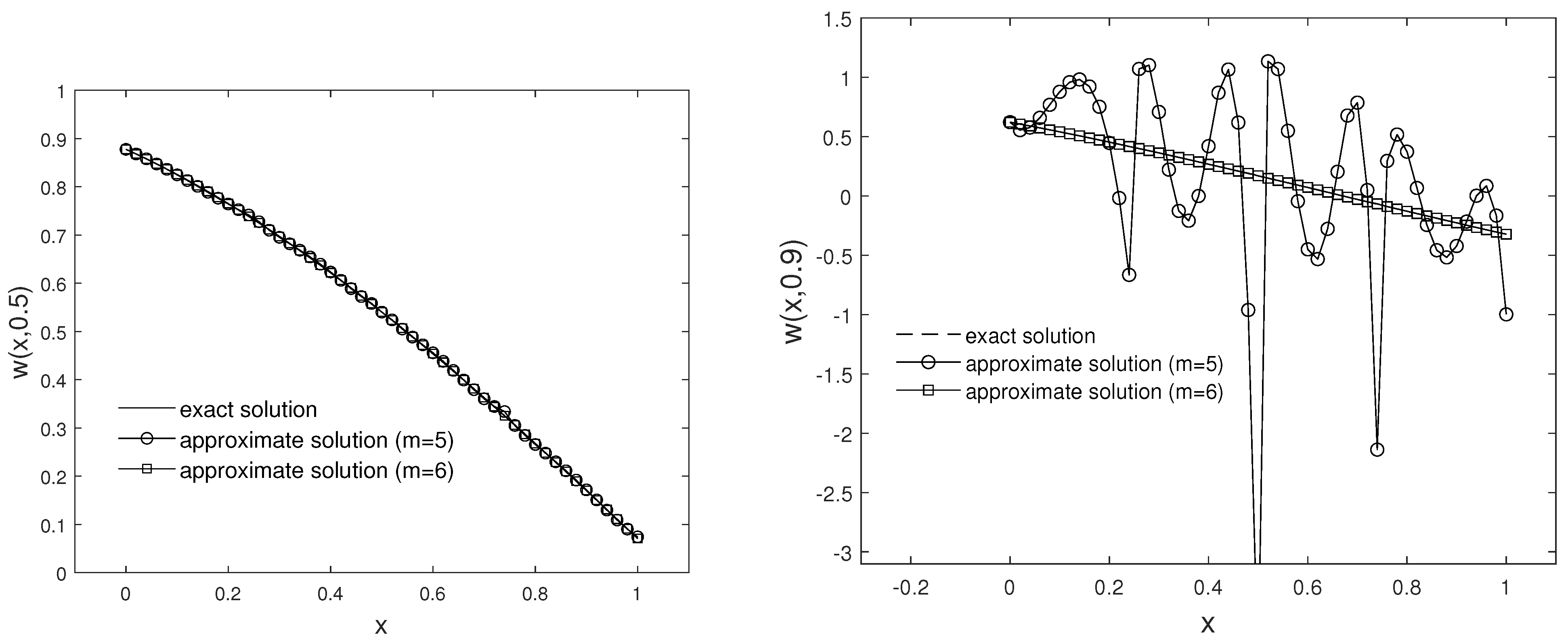
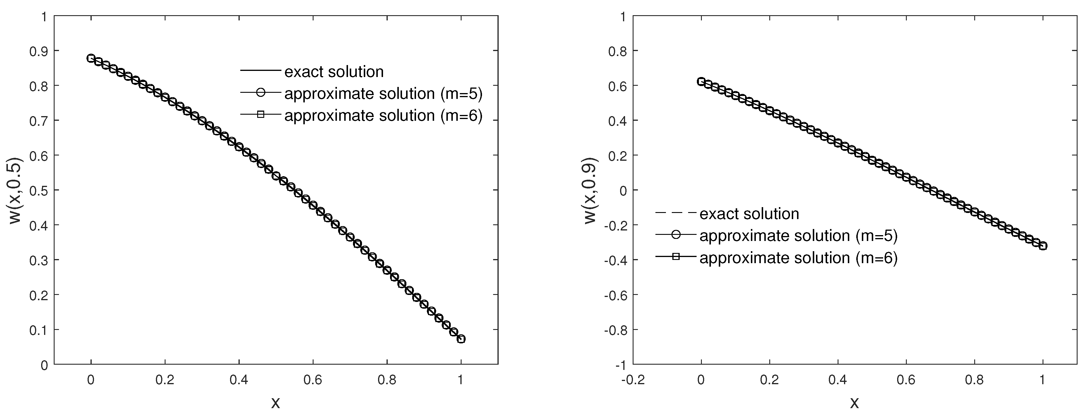
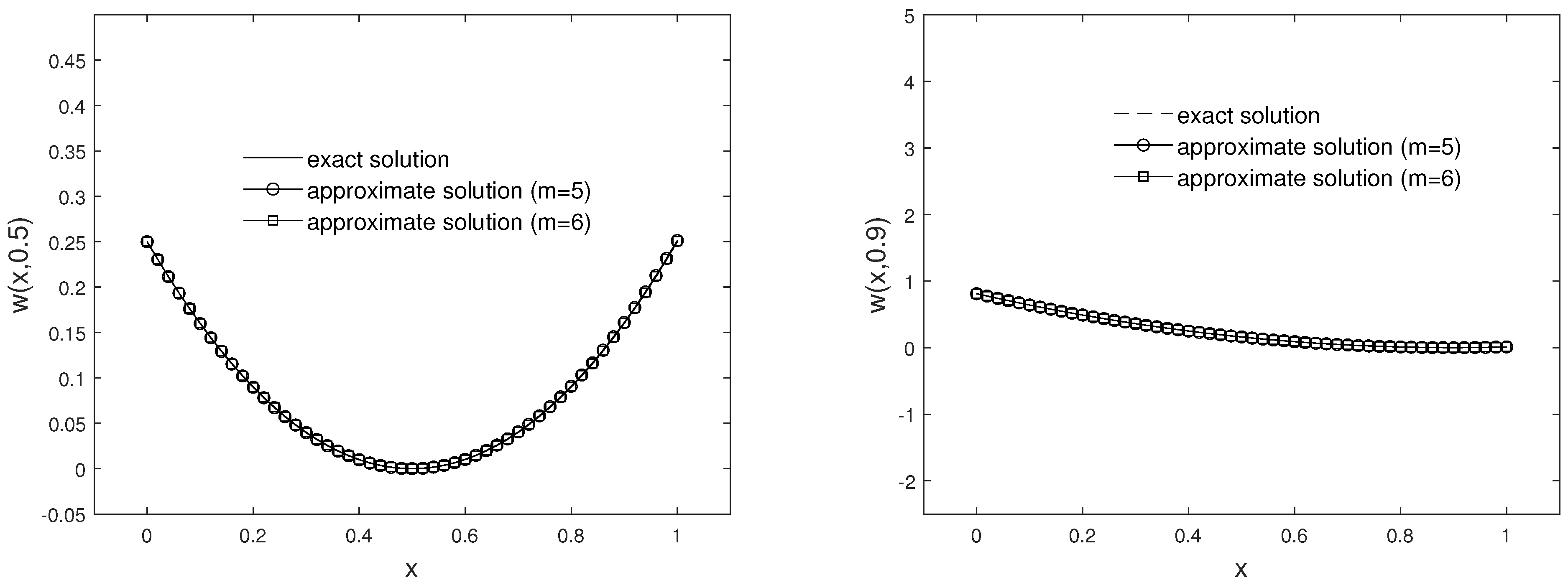
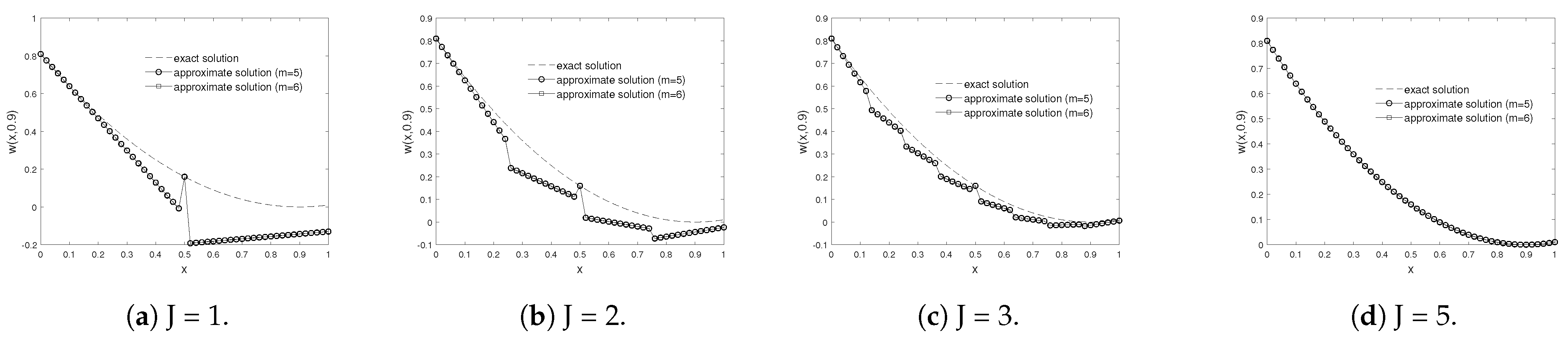
Example 1.

Let us dedicate the first example to the case that the desired Equation (1) is of form

$$w_t(x,t)+w_x(x,t)+w(x,t)=-2sin(x+t)+cos(x+t),$$

with boundary and initial conditions

$$w(x,0)=cos\left(x\right),x\in [0,1],w(0,t)=cos\left(t\right),t\in [0,T].$$

One can find the exact solution that is reported in [6]

$$w(x,t)=cos(x+t).$$

Table 1. Comparison of $L_2$–error computed using explicit, implicit and Crank–Nicolson methods with time step size $\delta t=0.1/2^{m-1}$ for Example 1.

$\mathit{\theta }$	$\mathit{m}=1$	$\mathit{m}=2$	$\mathit{m}=3$	$\mathit{m}=4$	$\mathit{m}=5$	$\mathit{m}=6$	$\mathit{m}=7$	$\mathit{m}=8$	$\mathit{m}=9$	$\mathit{m}=10$
0	$1.18\times {10}^4$	$4.33\times {10}^6$	$3.10\times {10}^7$	$7.57\times {10}^4$	$2.95$	$1.22\times {10}^{-3}$	$1.39\times {10}^{-4}$	$6.80\times {10}^{-5}$	$3.39\times {10}^{-5}$	$1.69\times {10}^{-5}$
$1/2$	$3.4\times {10}^{-2}$	$1.7\times {10}^{-2}$	$8.5\times {10}^{-3}$	$4.2\times {10}^{-3}$	$2.1\times {10}^{-3}$	$1.0\times {10}^{-3}$	$5.1\times {10}^{-4}$	$2.5\times {10}^{-4}$	$1.3\times {10}^{-4}$	$8.2\times {10}^{-5}$
1	$5.8\times {10}^{-2}$	$2.9\times {10}^{-2}$	$1.5\times {10}^{-2}$	$7.3\times {10}^{-3}$	$3.7\times {10}^{-3}$	$1.8\times {10}^{-3}$	$9.0\times {10}^{-4}$	$4.4\times {10}^{-4}$	$2.1\times {10}^{-4}$	$1.1\times {10}^{-4}$

describes the comparison of $L_2$-error via explicit, implicit and Crank–Nicolson methods with time step size $\delta t=0.1/2^{m-1}$, $m=1,\cdots ,10$. It is quite obvious that the error tends to zero with increasing m.

Table 2. $L^2$ norm of errors taking $r=5$, $J=2$, $\theta =1/2$ and $\delta t=0.1/2^{m-1}$ for Example 1.

m	$\mathit{t}=0.2$	$\mathit{t}=0.4$	$\mathit{t}=0.6$	$\mathit{t}=0.8$	$\mathit{t}=1.0$
2	$9.07\times {10}^{-3}$	$1.50\times {10}^{-2}$	$1.80\times {10}^{-2}$	$1.86\times {10}^{-2}$	$1.71\times {10}^{-2}$
4	$2.27\times {10}^{-3}$	$3.74\times {10}^{-3}$	$4.50\times {10}^{-3}$	$4.63\times {10}^{-3}$	$4.24\times {10}^{-3}$
6	$5.67\times {10}^{-4}$	$9.34\times {10}^{-4}$	$1.12\times {10}^{-3}$	$1.16\times {10}^{-3}$	$1.06\times {10}^{-3}$
8	$1.42\times {10}^{-4}$	$2.34\times {10}^{-4}$	$2.81\times {10}^{-4}$	$2.89\times {10}^{-4}$	$2.65\times {10}^{-4}$
10	$3.54\times {10}^{-5}$	$5.84\times {10}^{-5}$	$7.02\times {10}^{-5}$	$7.23\times {10}^{-5}$	$6.63\times {10}^{-5}$

consists of $L_2$ norm of Example 1 at different values of time. The $L_2$-error graph of the explicit, implicit, and Crank–Nicolson methods taking different values for J when $r=3$ are shown in Figure 1. Figure 2 illustrates the approximate solution and absolute error taking $r=5$ and $J=2$ at time $t=1$.

Table 3. Absolute values of the error at the selected points taking $\theta =1/2$ and $\delta t=0.1/2^9$ for Example 1.

	Reference [7] $(\mathit{M}={\mathit{M}}^{\prime }=4)$		Reference [18] $(\mathit{N}=4)$	Proposed Method
$(\mathit{x},\mathit{t})$	Legendre Wavelets	Chebyshev Wavelet		$\mathit{r}=4,\mathit{J}=1$
$(0.1,0.1)$	$4.86\times {10}^{-5}$	$3.0\times {10}^{-4}$	$3.220\times {10}^{-5}$	$5.332\times {10}^{-6}$
$(0.2,0.2)$	$2.78\times {10}^{-4}$	$2.0\times {10}^{-4}$	$6.650\times {10}^{-5}$	$6.791\times {10}^{-6}$
$(0.3,0.3)$	$8.64\times {10}^{-5}$	$1.0\times {10}^{-4}$	$1.357\times {10}^{-4}$	$4.366\times {10}^{-5}$
$(0.4,0.4)$	$1.15\times {10}^{-4}$	$5.0\times {10}^{-4}$	$1.332\times {10}^{-4}$	$1.505\times {10}^{-4}$
$(0.5,0.5)$	$1.42\times {10}^{-4}$	$6.0\times {10}^{-4}$	$5.200\times {10}^{-5}$	$1.509\times {10}^{-4}$
$(0.6,0.6)$	$5.40\times {10}^{-6}$	$2.0\times {10}^{-4}$	$7.700\times {10}^{-5}$	$1.992\times {10}^{-4}$
$(0.7,0.7)$	$1.67\times {10}^{-4}$	$2.0\times {10}^{-4}$	$1.960\times {10}^{-4}$	$2.098\times {10}^{-4}$
$(0.8,0.8)$	$2.46\times {10}^{-4}$	$2.0\times {10}^{-4}$	$2.428\times {10}^{-4}$	$2.034\times {10}^{-4}$
$(0.9,0.9)$	$2.29\times {10}^{-4}$	$1.0\times {10}^{-4}$	$1.776\times {10}^{-4}$	$2.119\times {10}^{-4}$

displays absolute values of the error at the selected points by using the presented method taking $r=4$, $J=1$, $\theta =1/2$ and $\delta t=0.1/2^9$. The results have been compared with the Legendre wavelets and Chebyshev wavelet collocation method [7], and also Bernoulli matrix approach [18]. To confirm the stability condition that we obtained in Section 3.1, Figure 3 and Figure 4 and

Table 4. $L^2$ norm of errors taking $r=5$, $J=2$, $\theta =1/2$ and $\delta t=0.1/2^{m-1}$ for Example 1.

m	$\mathit{\theta }=0$	$\mathit{\theta }=0.5$	$\mathit{\theta }=1$
1	$2.74556398$	$0.99667345$	$0.95750928$
2	$1.96489325$	$0.99446140$	$0.97722388$
3	$1.45253127$	$0.99335639$	$0.98830702$
4	$1.16631074$	$0.99488512$	$0.99408949$
5	$1.04801504$	$0.99716602$	$0.99704939$
6	$1.01190091$	$0.99850952$	$0.99855537$
7	$1.00262776$	$0.99928905$	$0.99930055$
8	$1.00046389$	$0.99965462$	$0.99965498$
9	$1.00001839$	$0.99982309$	$0.99982817$
10	$0.99995576$	$0.99991242$	$0.99991142$

are considered. One can observe that when the spectral radius of matrix $A^{-1}B$ is less than 1, the proposed method is stable. In view of Figure 3 and Figure 4, the explicit method at $m=10$ becomes stable while the Crank–Nicolson method is stable from $m=1$. We have the same result for the implicit method $(\theta =1)$.

Example 2.

As the second example, let us consider the HPDEs (1) so that $a_1=1$, $a_2=1$ and

$$f(x,t)={(x-t)}^2,$$

with boundary and initial conditions given by

$$w(x,0)=x^2,x\in [0,1],w(0,t)=t^2,t\in [0,T].$$

For this example, we have the exact solution [7]

$$w(x,t)={(x-t)}^2.$$

Table 5. $L_2$–error comparison among explicit, implicit, and Crank–Nicolson methods with time step size $\delta t=0.1/2^{m-1}$ for Example 2.

$\mathit{\theta }$	$\mathit{m}=1$	$\mathit{m}=2$	$\mathit{m}=3$	$\mathit{m}=4$	$\mathit{m}=5$	$\mathit{m}=6$	$\mathit{m}=7$	$\mathit{m}=8$	$\mathit{m}=9$	$\mathit{m}=10$
0	$2.37\times {10}^4$	$8.67\times {10}^6$	$6.20\times {10}^7$	$1.51\times {10}^5$	$5.88\times {10}^{-0}$	$2.68\times {10}^{-3}$	$6.44\times {10}^{-4}$	$3.21\times {10}^{-4}$	$1.60\times {10}^{-4}$	$8.01\times {10}^{-5}$
$1/2$	$1.45\times {10}^{-2}$	$7.25\times {10}^{-3}$	$3.62\times {10}^{-3}$	$1.81\times {10}^{-3}$	$9.06\times {10}^{-4}$	$4.53\times {10}^{-4}$	$2.27\times {10}^{-4}$	$1.13\times {10}^{-4}$	$5.66\times {10}^{-5}$	$2.83\times {10}^{-5}$
1	$2.46\times {10}^{-2}$	$1.23\times {10}^{-2}$	$6.13\times {10}^{-3}$	$3.06\times {10}^{-3}$	$1.53\times {10}^{-3}$	$7.65\times {10}^{-4}$	$3.82\times {10}^{-4}$	$1.91\times {10}^{-4}$	$9.55\times {10}^{-5}$	$4.78\times {10}^{-5}$

shows the comparison of $L_2$-error via explicit, implicit and Crank–Nicolson methods with time step size $\delta t=0.1/2^{m-1}$, $m=1,\cdots ,10$, $r=5$ and $J=2$.

Table 6. $L^2$ norm of errors taking $r=3$, $J=2$, $\theta =1/2$ and $\delta t=0.1/2^{m-1}$ for Example 2.

m	$\mathit{t}=0.2$	$\mathit{t}=0.4$	$\mathit{t}=0.6$	$\mathit{t}=0.8$	$\mathit{t}=1.0$
2	$3.75\times {10}^{-3}$	$4.50\times {10}^{-3}$	$3.97\times {10}^{-3}$	$4.58\times {10}^{-3}$	$7.27\times {10}^{-3}$
4	$9.37\times {10}^{-4}$	$1.12\times {10}^{-3}$	$9.91\times {10}^{-4}$	$1.14\times {10}^{-3}$	$1.82\times {10}^{-3}$
6	$2.34\times {10}^{-4}$	$2.81\times {10}^{-4}$	$2.48\times {10}^{-4}$	$2.86\times {10}^{-4}$	$4.55\times {10}^{-4}$
8	$5.85\times {10}^{-5}$	$7.02\times {10}^{-5}$	$6.20\times {10}^{-5}$	$7.15\times {10}^{-5}$	$1.14\times {10}^{-4}$
10	$1.46\times {10}^{-5}$	$1.76\times {10}^{-5}$	$1.55\times {10}^{-5}$	$1.79\times {10}^{-5}$	$2.84\times {10}^{-5}$

consists of $L_2$ norm of Example 2 at different values of time. Figure 5 illustrates the approximate solution and absolute error taking $r=5$ and $J=2$ at time $t=1$. Figure 6 shows the $L_2$-error using explicit method and implicit method taking $r=3$ and $J=2$ at time $\delta t=0.1/2^{m-1}$, $m=1,\dots ,10$. Figure 7, Figure 8 and Figure 9 confirm our investigation about stability. According to stability investigation, if the spectral radius of matrix $A^{-1}B$ is not less than 1, then the time discretization leads to divergence when t increases. To reduce this effect, we must increase the time steps. In

Table 7. Absolute values of the error at the selected points taking $\theta =1/2$ and $\delta t=0.1/2^9$ for Example 2.

	Reference [7] $(\mathit{M}={\mathit{M}}^{\prime }=4)$		Proposed Method
$(\mathit{x},\mathit{t})$	Legendre Wavelets	Chebyshev Wavelet	$\mathit{r}=4,\mathit{J}=1$
$(0.1,0.1)$	$1.03\times {10}^{-4}$	$2.57\times {10}^{-4}$	$1.11\times {10}^{-7}$
$(0.2,0.2)$	$9.00\times {10}^{-6}$	$3.83\times {10}^{-4}$	$1.09\times {10}^{-7}$
$(0.3,0.3)$	$5.87\times {10}^{-5}$	$4.38\times {10}^{-4}$	$5.88\times {10}^{-7}$
$(0.4,0.4)$	$9.94\times {10}^{-5}$	$2.22\times {10}^{-5}$	$1.30\times {10}^{-6}$
$(0.5,0.5)$	$1.12\times {10}^{-4}$	$2.30\times {10}^{-4}$	$2.58\times {10}^{-6}$
$(0.6,0.6)$	$9.94\times {10}^{-5}$	$1.38\times {10}^{-5}$	$7.09\times {10}^{-7}$
$(0.7,0.7)$	$5.87\times {10}^{-5}$	$3.66\times {10}^{-4}$	$3.69\times {10}^{-7}$
$(0.8,0.8)$	$9.00\times {10}^{-6}$	$2.75\times {10}^{-4}$	$3.73\times {10}^{-8}$
$(0.9,0.9)$	$1.03\times {10}^{-4}$	$4.01\times {10}^{-4}$	$2.47\times {10}^{-7}$

the results have been compared with the Legendre wavelets and Chebyshev wavelet collocation method [7]. It shows that the proposed method offers better accuracy using the same multiplicity parameter r and refinement level J. In Figure 10, we show the effect of refinement level J and time step size $\delta t$ on absolute error. In addition, this figure confirms our investigation about consistency.

5. Conclusions

This work is devoted to solving the one-dimensional partial differential equation with boundary and initial conditions. To this end, the desired equation reduces to an ordinary differential equation using the $\theta$-weighted method. This ODE is solved by employing the Galerkin method based on the interpolating scaling functions. The stability, consistency, and convergency of the method are investigated. The numerical examples are reported to illustrate the accuracy and efficiency of the method. The results show that three parameters are important here: the $\theta$ parameter that changes the $\theta$-weighted method, the $\delta t$ parameter that controls the time steps, and the refinement level J. The results show that, using the proposed method, better results are obtained compared to similar methods. Among the methods utilized in this paper, the implicit and Crank–Nicolson methods are stable methods that need fewer steps than the explicit method to achieve proper accuracy.

References

- Dehghan, M. A computational study of the one-dimensional parabolic equation subject to nonclassical boundary specifications. Numer. Methods Partial Differ. Equ. 2006, 22, 220–257. [Google Scholar] [CrossRef]
- Dehghan, M.; Shokri, A. A numerical method for solving the hyperbolic telegraph equation. Numer. Methods Partial Differ. Equ. 2008, 24, 1080–1093. [Google Scholar] [CrossRef]
- Lakestani, M.; Saray, B.N. Numerical solution of telegraph equation using interpolating scaling functions. Comput. Math. Appl. 2010, 60, 1964–1972. [Google Scholar] [CrossRef]
- Jebreen, H.B.; Cano, Y.C.; Dassios, I. An efficient algorithm based on the multi-wavelet Galerkin method for telegraph equation. AIMS Math. 2021, 6, 1296–1308. [Google Scholar] [CrossRef]
- Doha, E.H.; Bhrawy, A.H.; Hafez, R.M.; Abdelkawy, M.A. A Chebyshev–Gauss-Radau scheme for nonlinear hyperbolic system of first order. Appl. Math. Inf. Sci. 2014, 8, 535–544. [Google Scholar] [CrossRef]
- Doha, E.H.; Hafez, R.M.; Youssri, Y.H. Shifted Jacobi spectral-Galerkin method for solving hyperbolic partial differential equations. Comput. Math. Appl. 2019, 78, 889–904. [Google Scholar] [CrossRef]
- Singh, S.; Patel, V.K.; Singh, V.K. Application of wavelet collocation method for hyperbolic partial differential equations via matrices. Appl. Math. Comput. 2018, 320, 407–424. [Google Scholar] [CrossRef]
- Dehghan, M.; Lakesatani, M. The Use of Cubic B-Spline Scaling Functions for Solving the One-dimensional Hyperbolic Equation with a Nonlocal Conservation Condition. Numer. Methods Partial Differ. Equ. 2007, 23, 1277–1289. [Google Scholar] [CrossRef]
- Bougoffa, L. An efficient method for solving nonlocal initial-boundary value problems for linear and nonlinear first-order hyperbolic partial differential equations. J. Appl. Math. Comput. 2013, 43, 31–54. [Google Scholar] [CrossRef]
- Saadatmandi, A.; Dehghan, M. Numerical solution of hyperbolic telegraph equation using the Chebyshev Tau method. Numer. Methods Partial Differ. Equ. 2010, 26, 239–252. [Google Scholar] [CrossRef]
- Alpert, B.; Beylkin, G.; Gines, D.; Vozovoi, L. Adaptive solution of partial differential equations in multiwavelet bases. J. Comput. Phys. 2002, 182, 149–190. [Google Scholar] [CrossRef]
- Saray, B.N. Sparse multiscale representation of Galerkin method for solving linear-mixed Volterra-Fredholm integral equations. Math. Methods Appl. Sci. 2020, 43, 2601–2614. [Google Scholar] [CrossRef]
- Alpert, B.; Beylkin, G.; Coifman, R.R.; Rokhlin, V. Wavelet-like bases for the fast solution of second-kind integral equations. SIAM J. Sci. Statist. Comput. 1993, 14, 159–184. [Google Scholar] [CrossRef]
- Seyedi, S.H.; Saray, B.N.; Ramazani, A. High-Accuracy Multiscale Simulation of Three-Dimensional Squeezing Carbon Nanotube-Based Flow inside a Rotating Stretching Channel. Math. Prob. Eng. 2019, 2019, 9890626. [Google Scholar] [CrossRef]
- Saray, B.N.; Manafian, J. Sparse representation of delay differential equation of pantograph type using multiwavelets Galerkin method. Eng. Comput. 2018, 35, 887–903. [Google Scholar] [CrossRef]
- Shahriari, M.; Saray, B.N.; Lakestani, M.; Manafian, J. Numerical treatment of the Benjamin-Bona-Mahony equation using Alpert multiwavelets. Eur. Phys. J. Plus 2018, 133, 201. [Google Scholar] [CrossRef]
- Morton, K.W.; Mayers, D.F. Numerical Solution of Partial Differential Equations an Introduction, 2nd ed.; Cambridge University Press: Cambridge, UK; New York, NY, USA, 2005. [Google Scholar]
- Tohidi, E.; Toutounian, F. Convergence analysis of Bernoulli matrix approach for one-dimensional matrix hyperbolic equations of the first order. Comput. Math. Appl. 2014, 68, 1–12. [Google Scholar] [CrossRef]
Figure 1.
Plot of –errors at time taking and for Example 1.
Figure 2.
Plot of the approximate solution (left) and errors (right) taking and for Example 1.
Figure 3.
Plot of exact and approximate solutions at time and taking , , and for Example 1.
Figure 4.
Figure 5.
Plot of the approximate solution (left) and errors (right) taking and for Example 2.
Figure 6.
—error using explicit method (left) and implicit error (right) taking and at time for Example 2.
Figure 7.
Plot of exact and approximate solutions at time and taking , , and for Example 2.
Figure 8.
Figure 9.
Figure 10.
Effect of the refinement level J and on the absolute error for Example 2.