Wiener Complexity versus the Eccentric Complexity

Abstract

Let $w_G\left(u\right)$ be the sum of distances from u to all the other vertices of G. The Wiener complexity, $C_W\left(G\right)$, is the number of different values of $w_G\left(u\right)$ in G, and the eccentric complexity, $C_{\mathrm{ec}}\left(G\right)$, is the number of different eccentricities in G. In this paper, we prove that for every integer c there are infinitely many graphs G such that $C_W\left(G\right)-C_{\mathrm{ec}}\left(G\right)=c$. Moreover, we prove this statement using graphs with the smallest possible cyclomatic number. That is, if $c\ge 0$ we prove this statement using trees, and if $c<0$ we prove it using unicyclic graphs. Further, we prove that $C_{\mathrm{ec}}\left(G\right)\le 2C_W\left(G\right)-1$ if G is a unicyclic graph. In our proofs we use that the function $w_G\left(u\right)$ is convex on paths consisting of bridges. This property also promptly implies the already known bound for trees $C_{\mathrm{ec}}\left(G\right)\le C_W\left(G\right)$. Finally, we answer in positive an open question by finding infinitely many graphs G with diameter 3 such that $C_{\mathrm{ec}}\left(G\right)<C_W\left(G\right)$.

1. Introduction

Let G be a graph. Denote by $V\left(G\right)$ and $E\left(G\right)$ its vertex and edge sets, respectively. If $u\in V\left(G\right)$, then ${deg}_G\left(u\right)$ denotes the degree of u in G, and if $S\subseteq V\left(G\right)$ then $N\left(S\right)$ denotes the set S together with the vertices which have a neighbour in S. Obviously, $\left|N\left(u\right)\right|={deg}_G\left(u\right)+1$. If $R\subseteq E\left(G\right)$ then $G-R$ denotes a graph obtained when we remove all the edges of R from G. Similarly, if $S\subseteq V\left(G\right)$ then $G-S$ denotes a graph obtained when we remove all the vertices of S and all edges incident with a vertex of S from G. An edge $e\in E\left(G\right)$ is a bridge if $G-\left\{e\right\}$ has more components than G.

If $u,v\in V\left(G\right)$ then ${\mathrm{dist}}_G(u,v)$ is the length of a shortest path from u to v in G. The longest distance from a vertex u is its eccentricity $e_G\left(u\right)$. Hence, $e_G\left(u\right)=max\{{\mathrm{dist}}_G(u,v);v\in V\left(G\right)\}$. Using the eccentricity we define the radius $\mathrm{rad}\left(G\right)=min\{e_G\left(u\right);u\in V\left(G\right)\}$, and the diameter $\mathrm{diam}\left(G\right)=max\{e_G\left(u\right);u\in V\left(G\right)\}=max\{{\mathrm{dist}}_G(u,v);u,v\in V\left(G\right)\}$. The eccentric complexity of G is defined as

$$C_{\mathrm{ec}}\left(G\right)=\left|\{e_G\left(u\right);u\in V\left(G\right)\}\right|.$$

Observe that $C_{\mathrm{ec}}\left(G\right)=\mathrm{diam}\left(G\right)-\mathrm{rad}\left(G\right)+1$. The eccentric complexity has been introduced in [1]. Also see [2] for related connective eccentric complexity.

On the other hand the Wiener complexity of G is

$$C_W\left(G\right)=\left|\{w_G\left(u\right);u\in V\left(G\right)\}\right|,$$

where $w_G\left(u\right)={\sum }_{v\in V\left(G\right)}\mathrm{dist}(u,v)$ is the transmission of u in G. The parameter $\frac{1}{2}{\sum }_{u\in V\left(G\right)}{w}_G\left(u\right)$ is known as the Wiener index $W\left(G\right)$. Hence, $W\left(G\right)={\sum }_{u,v\in V\left(G\right)}\mathrm{dist}(u,v)$. The Wiener complexity $C_W\left(G\right)$ of a graph G was introduced in [3]. Further research on $C_W\left(G\right)$ can be found in [4,5,6]. For results on Wiener index see, e.g., [7].

In [8] the authors study the relation between $C_{\mathrm{ec}}\left(G\right)$ and $C_W\left(G\right)$. They prove the following statement.

Theorem 1.

If T is a tree then $C_{\mathrm{ec}}\left(T\right)\le C_W\left(T\right)$.

Next, using cartesian products they prove that for every $c\ge 0$ there are graphs G with $C_W\left(G\right)-C_{\mathrm{ec}}\left(G\right)=c$ and for every $k>0$ there are graphs G with $C_{\mathrm{ec}}\left(G\right)-C_W\left(G\right)=2^k$. Here we continue in their research. We prove that for every $c\ge 0$ there are infinitely many trees T such that $C_W\left(T\right)-C_{\mathrm{ec}}\left(T\right)=c$. By Theorem 1 to construct graphs G with $C_{\mathrm{ec}}\left(G\right)>C_W\left(G\right)$ we must abandon the class of trees. So we concentrate on graphs with cyclomatic number 1. We prove that for every $c>0$ there are infinitely many unicyclic graphs G such that $C_{\mathrm{ec}}\left(G\right)-C_W\left(G\right)=c$.

All graphs G with $C_{\mathrm{ec}}\left(G\right)<C_W\left(G\right)$ found in [8] have diameter at least 4, and it was shown that there are no such graphs of diameter at most 2. So the authors posed in [8] the following problem.

Problem 1.

Does there exist a graph G with diameter 3 and $C_{\mathrm{ec}}\left(G\right)>C_W\left(G\right)$?

We answer Problem 1 affirmatively and we find infinitely many graphs satisfying its requirements.

The outline of the paper is as follows. In Section 2 we characterize all pairs $c_1$ and $c_2$ such that there is a tree T with $C_{\mathrm{ec}}\left(T\right)=c_1$ and $C_W\left(T\right)=c_2$. Analogously, in Section 3 we characterize all pairs $c_1$ and $c_2$ such that $c_1<c_2$ and there is a unicyclic graph G with $C_W\left(G\right)=c_1$ and $C_{\mathrm{ec}}\left(G\right)=c_2$. Finally, in Section 4 we deal with Problem 1.

2. Trees

In this section we characterize pairs $c_1$ and $c_2$ such that there are (infinitely many) trees T with $C_{\mathrm{ec}}\left(T\right)=c_1$ and $C_W\left(T\right)=c_2$. To do this, first we show that $w_T$ is a strictly convex function on paths consisting of bridges; observe that in a tree, every edge is a bridge. However, firstly we state the following easy lemma.

Lemma 1.

Let G be a connected graph with a bridge $u_1{u}_2$. Let $G_1$ and $G_2$ be the two components of $G-u_1{u}_2$, such that $u_i\in V\left(G_i\right)$, $1\le i\le 2$, and let $n_i$ be the number of vertices in $G_i$. Then $w_G\left(u_1\right)-w_G\left(u_2\right)=n_2-n_1$.

Proof. 

Let $w_i$ be the transmission of $u_i$ in $G_i$, $1\le i\le 2$. Then

$$w_G\left(u_1\right)=w_1+n_2+w_2\mathrm{and}{w}_G\left(u_2\right)=n_1+w_1+w_2.$$

Hence, $w_G\left(u_1\right)-w_G\left(u_2\right)=n_2-n_1$. □

Recall that a function $f\left(i\right)$ defined on $\{0,1,\dots ,t\}$ is strictly convex, if for every $i\in \{1,\dots ,t-1\}$, we have $2f\left(i\right)<f(i-1)+f(i+1)$, or equivalently $f\left(i\right)-f(i-1)<f(i+1)-f\left(i\right)$. We have the following statement.

Lemma 2.

Let G be a graph. Further, let $P=v_0{v}_1\dots v_t$ be a path in G such that every edge of P is a bridge. Then $f\left(i\right)=w_G\left(v_i\right)$ is a strictly convex function on $\{0,1,\dots ,t\}$.

Proof. 

Let $u_1{u}_2{u}_3$ be a subpath of P. Then $G-\{u_1{u}_2,u_2{u}_3\}$ has three components. Denote by $G_i$ the component of $G-\{u_1{u}_2,u_2{u}_3\}$ which contains $u_i$, for each $i\in \{1,2,3\}$. Moreover, denote $s_i=\left|V\left(G_i\right)\right|$. By Lemma 1, we have

$$w_G\left(u_1\right)+w_G\left(u_3\right)-2w_G\left(u_2\right)=(s_2+s_3-s_1)+(s_1+s_2-s_3)=2s_2>0.$$

Consequently, $f\left(i\right)=w_G\left(v_i\right)$ is strictly convex on $\{0,1,\dots ,t\}$. □

Observe that considering a diametric path, Lemma 2 directly implies Theorem 1. However, we use it in the following statement which characterizes all possible pairs $C_{\mathrm{ec}}\left(T\right)$, $C_W\left(T\right)$ for trees.

Theorem 2.

It holds:

(i) 

If $3\le c_1\le c_2$ then there are infinitely many trees T with $C_{\mathrm{ec}}\left(T\right)=c_1$ and $C_W\left(T\right)=c_2$.

(ii) 

If $c_1=2$ and $c_2\in \{2,4\}$ then there are infinitely many trees T with $C_{\mathrm{ec}}\left(T\right)=c_1$ and $C_W\left(T\right)=c_2$ and no trees with $C_{\mathrm{ec}}\left(T\right)=c_1$ and $C_W\left(T\right)\notin \{2,4\}$.

(iii) 

If $c_1=1$ then there are only two trees T with $C_{\mathrm{ec}}\left(T\right)=1$ and in this case $C_W\left(T\right)=1$ as well.

Proof. 

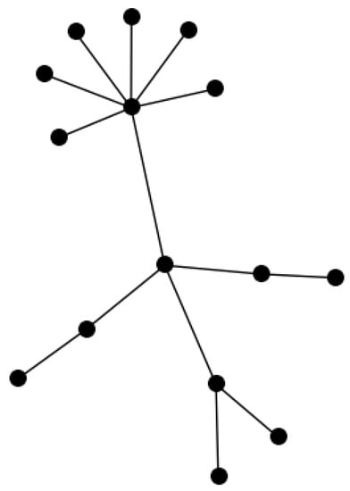
Consider $\left(i\right)$. Here $c_1\ge 3$. First suppose that $c_2>c_1$. Let $k=\lceil \frac{c_2-1}{c_1-1}\rceil$. Take k paths $P_0,P_1,\dots ,P_{k-1}$ of length $c_1-1$ and denote their vertices so that $P_i=v_{i,0}{v}_{i,1}\dots v_{i,c_1-1}$, where $0\le i\le k-1$. Denote

$$\ell =c_2-1-(⌈\frac{c_2-1}{c_1-1}⌉-1)(c_1-1).$$

Let $P_k$ be a path of length ℓ so that $P_k=v_{k,0}{v}_{k,1}\dots v_{k,\ell }$. Since $\lceil \frac{c_2-1}{c_1-1}\rceil (c_1-1)\ge (c_2-1)$, we have $\ell \le c_1-1$, and since $\lceil \frac{c_2-1}{c_1-1}\rceil (c_1-1)<(c_2-1)+(c_1-1)$, we have $\ell >0$. Thus, $1\le \ell \le c_1-1$. Now attach to $v_{i,c_1-2}$ exactly $i-1$ new pendant vertices, $2\le i\le k-1$, and attach to $v_{k,\ell -1}$ exactly $q-1$ new vertices. We expect that q is a big number. Finally, identify the vertices $v_{0,0},v_{1,0},\dots ,v_{k,0}$ into a single vertex, which we denote by c, and denote the resulting tree by T, see Figure 1. Observe that there is 1 pendant vertex attached to $v_{0,c_1-2}$ in T and exactly i pendant vertices are attached to $v_{i,c_1-2}$, $1\le i\le k-1$. Further, since $k\ge 2$ ($k\ge 1$ would suffice since there is also $P_0$) we have $\mathrm{rad}\left(T\right)=c_1-1$ and $\mathrm{diam}\left(T\right)=2(c_1-1)$, so that $C_{\mathrm{ec}}\left(T\right)=c_1$. Obviously, if u and v are pendant vertices attached to the same vertex in T then $w_T\left(u\right)=w_T\left(v\right)$. Also, $w_T\left(u\right)=w_T\left(v\right)$ if $u=v_{0,i}$ and $v=v_{1,i}$, $1\le i\le c_1-1$. In all other cases we show that $w_T\left(u\right)\ne w_T\left(v\right)$. Hence, we show that $c,v_{1,1},v_{1,2},\dots ,v_{k,\ell }$ have different transmissions.

Denote $r=c_1-1$. Let P be a path in T consisting of vertices of $P_a$ and $P_b$, $1\le a<b\le k-1$. Then $P=v_{a,r}\dots v_{a,1}c{v}_{b,1}\dots v_{b,r}$. Let $T^{\prime }$ be the nontrivial component of $T-\{v_{a,1},\dots ,v_{a,r},v_{b,1},\dots ,v_{b,r}\}$. Denote by $w^{\prime }$ the transmission of c in $T^{\prime }$ and denote by z the number of vertices of $T^{\prime }$. Then

$$\begin{array}{ccc}\hfill w_T\left(v_{a,r}\right)& =& 2(a-1)+\left(\genfrac{}{}{0pt}{}{2r+1}{2}\right)+2r(b-1)+w^{\prime }+(z-1)r;\hfill \\ \hfill w_T\left(v_{a,i}\right)& =& (r-i)(a-1)+\left(\genfrac{}{}{0pt}{}{r-i+1}{2}\right)+\left(\genfrac{}{}{0pt}{}{r+i+1}{2}\right)+(r+i)(b-1)+w^{\prime }+(z-1)i,1\le i\le r-1;\hfill \\ \hfill w_T\left(c\right)& =& r(a-1)+\left(\genfrac{}{}{0pt}{}{r+1}{2}\right)+\left(\genfrac{}{}{0pt}{}{r+1}{2}\right)+r(b-1)+w^{\prime };\hfill \\ \hfill w_T\left(v_{b,i}\right)& =& (r+i)(a-1)+\left(\genfrac{}{}{0pt}{}{r+i+1}{2}\right)+\left(\genfrac{}{}{0pt}{}{r-i+1}{2}\right)+(r-i)(b-1)+w^{\prime }+(z-1)i,1\le i\le r-1;\hfill \\ \hfill w_T\left(v_{b,r}\right)& =& 2r(a-1)+\left(\genfrac{}{}{0pt}{}{2r+1}{2}\right)+2(b-1)+w^{\prime }+(z-1)r.\hfill \end{array}$$

Since $w_T\left(v_{a,i}\right)-w_T\left(v_{b,i}\right)=(r-i)(a-b)+(r+i)(b-a)=2i(b-a)>0$ if $1\le i\le r-1$ and $w_T\left(v_{a,r}\right)-w_T\left(v_{b,r}\right)=(2r-2)(b-a)>0$, we have $w_T\left(v_{a,j}\right)>w_T\left(v_{b,j}\right)$, $1\le j\le r$. And since q and consequently also z are big, the terms containing z in the above expressions are crucial. Therefore $w_T\left(v_{a,1}\right)<w_T\left(v_{b,2}\right)$ and in general $w_T\left(v_{a,i}\right)<w_T\left(v_{b,i+1}\right)$, where $1\le i<r$. So we conclude that

$$w_T\left(c\right)<w_T\left(v_{b,1}\right)<w_T\left(v_{a,1}\right)<w_T\left(v_{b,2}\right)<w_T\left(v_{a,2}\right)<w_T\left(v_{b,3}\right)<\dots <w_T\left(v_{a,r}\right).$$

Now let P be a path consisting of $P_a$ and $P_k$, $1\le a\le k-1$. Then $P=v_{a,r}\dots v_{a,1}c{v}_{k,1}\dots v_{k,\ell }$$=u_{a+\ell }{u}_{a+\ell -1}\dots u_0$. We remark that $u_j$ are just different labels for vertices of P which will be used later. Similarly as above, let $T^{\prime }$ be the nontrivial component of $T-\{v_{a,1},\dots .v_{a,r},v_{k,1},\dots ,v_{k,\ell }\}$. Denote by $w^{\prime }$ the transmission of c in $T^{\prime }$ and denote by z the number of vertices of $T^{\prime }$. Then

$$\begin{array}{ccc}\hfill w_T\left(v_{a,r}\right)& =& 2(a-1)+\left(\genfrac{}{}{0pt}{}{r+\ell +1}{2}\right)+(r+\ell )(q-1)+w^{\prime }+(z-1)r;\hfill \\ \hfill w_T\left(v_{a,i}\right)& =& (r-i)(a-1)+\left(\genfrac{}{}{0pt}{}{r-i+1}{2}\right)+\left(\genfrac{}{}{0pt}{}{\ell +i+1}{2}\right)+(\ell +i)(q-1)+w^{\prime }+(z-1)i,1\le i\le r-1;\hfill \\ \hfill w_T\left(c\right)& =& r(a-1)+\left(\genfrac{}{}{0pt}{}{r+1}{2}\right)+\left(\genfrac{}{}{0pt}{}{\ell +1}{2}\right)+\ell (q-1)+w^{\prime };\hfill \\ \hfill w_T\left(v_{k,i}\right)& =& (r+i)(a-1)+\left(\genfrac{}{}{0pt}{}{r+i+1}{2}\right)+\left(\genfrac{}{}{0pt}{}{\ell -i+1}{2}\right)+(\ell -i)(q-1)+w^{\prime }+(z-1)i,1\le i\le \ell -1;\hfill \\ \hfill w_T\left(v_{k,\ell }\right)& =& (r+\ell )(a-1)+\left(\genfrac{}{}{0pt}{}{r+\ell +1}{2}\right)+2(q-1)+w^{\prime }+(z-1)\ell .\hfill \end{array}$$

Observe that $u_2=v_{k,\ell -2}$ if $\ell \ge 3$, $u_2=c$ if $\ell =2$ and $u_2=v_{a,1}$ if $\ell =1$. In any case, we have $w_T\left(v_{k,l}\right)-w_T\left(u_2\right)\ge \left(\genfrac{}{}{0pt}{}{r+\ell +1}{2}\right)-\left(\genfrac{}{}{0pt}{}{r+\ell -1}{2}\right)-\left(\genfrac{}{}{0pt}{}{2}{2}\right)>0$, and so $w_T\left(u_0\right)>w_T\left(u_2\right)$. And since q is big, analogously as above we conclude that

$$w_T\left(u_1\right)<w_T\left(u_2\right)<w_T\left(u_0\right)<w_T\left(u_3\right)<w_T\left(u_4\right)<\dots <w_T\left(u_{r+\ell }\right).$$

Let $S=\{c,v_{1,1},\dots ,v_{k,\ell }\}$. As shown above, vertices in S have pairwise different transmissions, while the vertices outside S have transmissions as some vertices in S. Since

$$\left|S\right|=1+(\lceil \frac{c_2-1}{c_1-1}\rceil -1)(c_1-1)+[c_2-1-(\lceil \frac{c_2-1}{c_1-1}\rceil -1)(c_1-1)]=c_2,$$

we have $C_W\left(T\right)=c_2$.

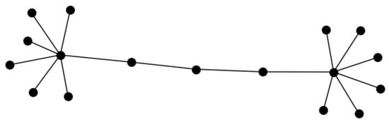
Now suppose $c_2=c_1$. Let $P=v_{0,c_1-1}\dots v_{0,1}c{v}_{1,1}\dots v_{1,c_1-1}$ be a path of length $2(c_1-1)$. We attach to both $v_{0,c_1-2}$ and $v_{1,c_1-2}$ exactly q pendant vertices and we denote by T the resulting tree, see Figure 2. Then T has $2c_1-1+2q$ vertices, $\mathrm{rad}\left(T\right)=c_1-1$ and $\mathrm{diam}\left(T\right)=2(c_1-1)$, so that $C_{\mathrm{ec}}\left(T\right)=c_1$. Denote $r=c_1-1$. By symmetry, we have $w_T\left(v_{0,i}\right)=w_T\left(v_{1,i}\right)$, $1\le i\le r$, and $w_T\left(u\right)=w_T\left(v\right)$ if u and v are pendant vertices of T. So it remains to show that the vertices $v_{0,r},\dots ,v_{0,1},c$ have different transmissions. However, since $w_T\left(v_{0,1}\right)=v_T\left(v_{1,1}\right)$, by Lemma 2 we get

$$w_T\left(c\right)<w_T\left(v_{0,1}\right)<\dots <v_T\left(v_{0,r}\right)$$

and so $C_W\left(T\right)=r+1=c_1$.

Now, consider $\left(ii\right)$. So, let $c_1=2$. If T is a tree with $\mathrm{rad}\left(T\right)\ge 3$, then $\mathrm{diam}\left(T\right)\ge 5$ and consequently $C_{\mathrm{ec}}\left(T\right)\ge 3$, a contradiction. Hence, either $\mathrm{rad}\left(T\right)=1$ and $\mathrm{diam}\left(T\right)=2$, in which case T is a star $K_{1,t}$, where $t\ge 2$, or $\mathrm{rad}\left(T\right)=2$ and $\mathrm{diam}\left(T\right)=3$, in which case T is a double star $D_{a,b}$, i.e., a graph on $a+b+2$ vertices obtained by attaching a pendant vertices to one vertex of $K_2$ and b pendant vertices to the other vertex of $K_2$, where $1\le a\le b$. If T is a star $K_{1,t}$, $t\ge 2$, then $C_W\left(T\right)=2$ since the central vertex has transmission smaller than is the transmission of pendant vertices. This establishes the case $c_1=c_2=2$. On the other hand if T is a double star then since pendant vertices adjacent to a common vertex have the same transmission, we have $C_W\left(T\right)\le 4$. In the next we consider $T=D_{a,b}$, where $a<b$, since $C_W\left(D_{a,a}\right)=2$, a case already solved by stars. Let $v_0,v_1,v_2,v_3$ be a path in $D_{a,b}$ such that ${deg}_T\left(v_1\right)=a+1$ and ${deg}_T\left(v_2\right)=b+1$. Then

$$\begin{array}{ccc}\hfill w_T\left(v_0\right)& =& 2(a-1)+3+3b;\hfill \\ \hfill w_T\left(v_1\right)& =& a+1+2b;\hfill \\ \hfill w_T\left(v_2\right)& =& 2a+1+b;\hfill \\ \hfill w_T\left(v_3\right)& =& 3a+3+2(b-1).\hfill \end{array}$$

Since $0<a<b$, it is obvious that $2a+1+b<a+1+2b<3a+1+2b<2a+1+3b$. Thus. $w_T\left(v_2\right)<w_T\left(v_1\right)<w_T\left(v_3\right)<w_T\left(v_0\right)$, and so $C_W\left(T\right)=4$.

Finally, consider $\left(iii\right)$. Since there are only two trees T such that $\mathrm{rad}\left(T\right)=\mathrm{diam}\left(T\right)$, namely the complete graphs $K_1$ and $K_2$, this part of Theorem 2 is trivial. □

Theorem 2 has the following consequence.

Corollary 1.

For every $c\ge 0$ there are infinitely many trees T such that $C_W\left(T\right)-C_{\mathrm{ec}}\left(T\right)=c$.

3. Unicyclic Graphs

In this section, we give counterparts of the previous results for unicyclic graphs. We also bound the eccentric complexity in term of Wiener complexity and characterize the pairs $c_1,c_2$ such that $c_1<c_2$ and there are (infinitely many) unicyclic graphs G with $C_W\left(G\right)=c_1$ and $C_{\mathrm{ec}}\left(G\right)=c_2$. We start with the following lemma.

Lemma 3.

Let G be a unicyclic graph with a cycle C. Further, let $u_2,v\in V\left(C\right)$ and let $u_1$ be a neighbour of $u_2$ which is not in C. If $w_G\left(u_1\right)\le w_G\left(u_2\right)$ then $w_G\left(u_2\right)<w_G\left(v\right)$.

Proof. 

Observe that $u_1{u}_2$ is a bridge in G. Hence, $G-u_1{u}_2$ has two components, say $G_1$ and $G_2$. Assume that $u_i\in V\left(G_i\right)$ and $n_i=\left|V\left(G_i\right)\right|$, $1\le i\le 2$. By the assumptions and by Lemma 1, $w_G\left(u_1\right)-w_G\left(u_2\right)=n_2-n_1\le 0$.

Let T be a tree obtained from G by removing an edge of C which is opposite (i.e., antipodal) to v. Observe that if C has odd length, then there is a unique edge opposite to v, while if C has even length, then there are two edges opposite to v. Obviously, $w_G\left(v\right)=w_T\left(v\right)$ and $w_G\left(u_2\right)\le w_T\left(u_2\right)$. Observe also that

$$0\ge w_G\left(u_1\right)-w_G\left(u_2\right)=w_T\left(u_1\right)-w_T\left(u_2\right).$$

Now, consider a path from $u_1$ to v in T. Assume that the length of this path is $k-1$ and denote their vertices by $u_1{u}_2{u}_3\dots u_k(=v)$. Since $u_1{u}_2$ is a bridge in T, we have $w_T\left(u_1\right)-w_T\left(u_2\right)=n_2-n_1$ again. And by Lemma 2 we get $w_T\left(u_1\right)+w_T\left(u_3\right)>2w_T\left(u_2\right)$ or equivalently $w_T\left(u_1\right)-w_T\left(u_2\right)>w_T\left(u_2\right)-w_T\left(u_3\right)$. Applying Lemma 2 several times we get

$$0\ge w_T\left(u_1\right)-w_T\left(u_2\right)>w_T\left(u_2\right)-w_T\left(u_3\right)>\dots >w_T\left(u_{k-1}\right)-w_T\left(v\right)$$

which implies $w_T\left(u_1\right)\le w_T\left(u_2\right)<w_T\left(u_3\right)<\dots <w_T\left(v\right)$ and consequently $w_G\left(u_2\right)\le w_T\left(u_2\right)<w_T\left(v\right)=w_G\left(v\right)$. □

The following statement characterizes all possible pairs $C_W\left(G\right)$, $C_{\mathrm{ec}}\left(G\right)$ for unicyclic graphs, provided that $C_W\left(G\right)<C_{\mathrm{ec}}\left(G\right)$.

Theorem 3.

Every unicyclic graph G satisfies

$$C_{\mathrm{ec}}\left(G\right)\le 2C_W\left(G\right)-1.$$

Moreover, for any positive integers $c_1$ and $c_2$ with $c_1<c_2\le 2c_1-1$ there are infinitely many unicyclic graphs G such that $C_W\left(G\right)=c_1$ and $C_{\mathrm{ec}}\left(G\right)=c_2$.

Proof. 

Let G be a unicyclic graph with a cycle C of length k. Further, let $P_1$ and $P_2$ be two longest paths starting in different vertices of C and which contain only edges which are not in C. Observe that if the length of $P_1$ is positive, then the path terminates in a pendant vertex of G. Similar statement holds for $P_2$. Let ${\ell }_i$ be the length of $P_i$, $1\le i\le 2$, and let $P_i=v_{i,0}{v}_{i,1}\dots v_{i,{\ell }_i}$, where $v_{i,0}\in V\left(C\right)$. Observe that in each of $P_1$ and $P_2$, there are at most two vertices with the same transmission, by Lemma 2. If there are three vertices, say $u_1$, $u_2$ and $u_3$, in $V\left(P_1\right)\cup V\left(P_2\right)$ which have the same transmission in G, then two of them are in one of the paths $P_1$ and $P_2$ while the third one is in the other. Without loss of generality we may assume that $u_1,u_2\in V\left(P_1\right)$ and $u_3\in V\left(P_3\right)$. Then $w_G\left(v_{1,1}\right)\le w_G\left(v_{1,0}\right)$ by Lemma 2, and so $w_G\left(v_{1,0}\right)<w_G\left(v_{2,0}\right)$ by Lemma 3. If $w_G\left(v_{2,1}\right)\le w_G\left(v_{2,0}\right)$ then $w_G\left(v_{2,0}\right)<w_G\left(v_{1,0}\right)$ by Lemma 3, a contradiction. Hence $w_G\left(v_{2,0}\right)<w_G\left(v_{2,1}\right)$, and by Lemma 2 $w_G\left(v_{2,0}\right)<w_G\left(v_{2,i}\right)$ for every i, $1\le i\le {\ell }_2$. Consequently $w_G\left(u_1\right)=w_G\left(u_2\right)\le w_G\left(v_{1,0}\right)<w_G\left(v_{2,0}\right)\le w_G\left(u_3\right)$. Hence, there are not three vertices in $V\left(P_1\right)\cup V\left(P_2\right)$ which have the same transmission in G. Therefore $C_W\left(G\right)\ge \lceil \frac{{\ell }_1+{\ell }_2}{2}\rceil +1$.

On the other hand $\mathrm{diam}\left(G\right)\le {\ell }_1+{\ell }_2+\lfloor k/2\rfloor$ and $\mathrm{rad}\left(G\right)\ge \lfloor k/2\rfloor$. So $C_{\mathrm{ec}}\left(G\right)=\mathrm{diam}\left(G\right)-\mathrm{rad}\left(G\right)+1\le {\ell }_1+{\ell }_2+1$, and hence

$$2C_W\left(G\right)-C_{\mathrm{ec}}\left(G\right)\ge 2⌈\frac{{\ell }_1+{\ell }_2}{2}⌉+2-l_1-l_2-1\ge 1.$$

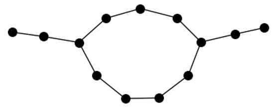
Now we prove the second result. Let $c_1$ and $c_2$ satisfy $c_1<c_2\le 2c_1-1$. Denote $\mathsf{\Delta }=c_2-c_1$. Let C be a cycle of length $4\mathsf{\Delta }$ and let $u_1$ and $v_1$ be opposite vertices on C. Attach to $u_1$ (resp. $v_1$) a path of length $c_1-1$$u_1{u}_2\dots u_{c_1}$ (resp. $v_1{v}_2\dots v_{c_1}$). Finally, attach to both $u_{c_1-1}$ and $v_{c_1-1}$ exactly $q\ge 0$ pendant vertices, and denote the resulting graph by G, see Figure 3.

Obviously, $\mathrm{diam}\left(G\right)=2(c_1-1)+2\mathsf{\Delta }=2c_2-2$. Since $c_2\le 2c_1-1$, we have $c_2-c_1\le c_1-1$, and so $2\mathsf{\Delta }\le \mathsf{\Delta }+(c_1-1)$. Thus, $\mathrm{rad}\left(G\right)=max\{\mathrm{rad}\left(C\right),\lceil \mathrm{diam}\left(G\right)/2\rceil \}=\mathsf{\Delta }+(c_1-1)$, which means that $C_{\mathrm{ec}}\left(G\right)=\mathrm{diam}\left(G\right)-\mathrm{rad}\left(G\right)+1=c_2$.

On the other hand, denote by $w^T$ the transmission of $u_1$ in the tree attached to C and denote by $w^C$ the transmission of $u_1$ in C. Then $w_G\left(u_1\right)=w^T+w^C+2\mathsf{\Delta }(c_1-1+q)+w^T$, and similarly for every vertex v of C we have $w_G\left(v\right)=2w^T+w^C+2\mathsf{\Delta }(c_1-1+q)$ as well. By Lemmas 2 and 3 it holds $w_G\left(u_1\right)<w_G\left(u_2\right)<\dots <w_G\left(u_{c_1}\right)$ and by symmetry $w_G\left(u_i\right)=w_G\left(v_i\right)$, $1\le i\le c_1$. Thus $C_W\left(G\right)=c_1$, and so G satisfies the assumptions of the theorem. □

Theorem 3 has the following consequence.

Corollary 2.

For every integer $c>0$ there are infinitely many unicyclic graphs G such that

$$C_{\mathrm{ec}}\left(G\right)-C_W\left(G\right)=c.$$

We remark that the attachment vertices $u_1$ and $u_2$ do not need to be opposite on C if $c_1$ is big enough (compared to $\mathsf{\Delta }=c_2-c_1$). We can use also even cycles of length $\not\equiv 0(mod4)$ and odd cycles, but again $c_1$ must be big enough. Though for small order graphs, one with even cycle are quite abundant, the smallest unicyclic graph G with a cycle of odd length satisfying $C_W\left(G\right)<C_{\mathrm{ec}}\left(G\right)$ has 13 vertices, and its cycle has length 9.

4. Graphs with Diameter 3

In this section we solve Problem 1. Observe that if $\mathrm{diam}\left(G\right)=3$ and $C_{\mathrm{ec}}\left(G\right)>C_W\left(G\right)$ then $\mathrm{rad}\left(G\right)=2$, $C_{\mathrm{ec}}\left(G\right)=2$ and $C_W\left(G\right)=1$. Hence, there is no unicyclic graph G satisfying the requirements of Problem 1, by Theorem 3.

Let G be a graph with diameter 3. For every vertex $u\in V\left(G\right)$, by $d_G^i\left(u\right)$ we denote the number of vertices of G which are at distance i from u. Denote ${\sigma }_G\left(u\right)=d_G^1\left(u\right)-d_G^3\left(u\right)$. We have the following statement.

Lemma 4.

Let G be a graph with diameter 3. Then $C_W\left(G\right)=1$ if and only if all vertices of G have the same value of σ.

Proof. 

Let $u\in V\left(G\right)$. Then $w_G\left(u\right)=d_G^1\left(u\right)+2d_G^2\left(u\right)+3d_G^3\left(u\right)$. Since $d_G^1\left(u\right)+d_G^2\left(u\right)+d_G^3\left(u\right)=n-1$, where $n=\left|V\right(G\left)\right|$, we have $d_G^2\left(u\right)=n-1-d_G^1\left(u\right)-d_G^3\left(u\right)$, and consequently $w_G\left(u\right)=2n-2-d_G^1\left(u\right)+d_G^3\left(u\right)$. Hence, if $v\in V\left(G\right)$ with $v\ne u$, then $w_G\left(v\right)=w_G\left(u\right)$ is equivalent with ${\sigma }_G\left(u\right)={\sigma }_G\left(v\right)$. □

By Lemma 4, in graphs G of diameter 3 with $C_{\mathrm{ec}}\left(G\right)=2$ and $C_W\left(G\right)=1$, the vertices of eccentricity 3 must have degree greater than is the degree of vertices of eccentricity 2. This looks surprising, nevertheless, there exist such graphs.

Let G be a graph on $2r$ vertices and let $S\subseteq V\left(G\right)$ such that $\left|S\right|=r$. By $A(G,S)$ we denote the graph obtained from G by adding two vertices, v and $v^{\prime }$, where v is connected to all vertices of S and $v^{\prime }$ is connected to all vertices of $V\left(G\right)\backslash S$. We have:

Proposition 1.

Let G be a k-regular graph of diameter 2 on $2(k+2)$ vertices. Moreover, let $S\subseteq V\left(G\right)$, $\left|S\right|=k+2$, such that every vertex of S has a neighbour in $V\left(G\right)\backslash S$ and every vertex of $V\left(G\right)\backslash S$ has a neighbour in S. Then $\mathrm{diam}\left(A\right(G,S\left)\right)=3$, $C_{\mathrm{ec}}\left(A(G,S)\right)=2$ and $C_W\left(A(G,S)\right)=1$.

Proof. 

First observe that $N_G\left(S\right)=V\left(G\right)=N_G(V\left(G\right)\backslash S)$. Since every vertex of S has a neighbour in $V\left(G\right)\backslash S$ and every vertex of $V\left(G\right)\backslash S$ has a neighbour in S, we have $e_{A(G,S)}\left(u\right)=2$ for every $u\in V\left(G\right)$. Since ${\mathrm{dist}}_{A(G,S)}(v,v^{\prime })=3$, we have $\mathrm{diam}\left(A\right(G,S\left)\right)=3$ and $C_{\mathrm{ec}}\left(A(G,S)\right)=2$.

If $u\in V\left(G\right)$ then ${deg}_{A(G,S)}\left(u\right)={\sigma }_{A(G,S)}\left(u\right)=k+1$. On the other hand ${deg}_{A(G,S)}\left(v\right)={deg}_{A(G,S)}\left(v^{\prime }\right)=k+2$. Moreover, since in G holds $N\left(S\right)=V\left(G\right)=N\left(V\right(G)\backslash S)$, we have $d_{A(G,S)}^3\left(v\right)=d_{A(G,S)}^3\left(v^{\prime }\right)=1$. Thus ${\sigma }_{A(G,S)}\left(v\right)={\sigma }_{A(G,S)}\left(v^{\prime }\right)=k+1$ and $C_W\left(A(G,S)\right)=1$, by Lemma 4. □

Since there is no 2-regular graph on 8 vertices with diameter 2, the smallest graph G satisfying assumptions of Proposition 1 is the Petersen graph in which S is the set of vertices of one of its 5-cycles. If G is the Petersen graph and S is the set of vertices of one of its 5-cycles, then $A(G,S)$ has 12 vertices.

However, there are also other graphs satisfying the assumptions of Proposition 1.

Lemma 5.

Let $k\ge 6$ be an even number, and let $D=\left(\right\{1,4,7,\dots \}\cap \{1,2,\dots ,k+1\left\}\right)\cup \{k+1,k,k-1,\dots ,i\}$ with $\left|D\right|=k/2$. Let G be the Cayley graph with $V\left(G\right)=Z_{2k+4}$ and $E\left(G\right)=\{ij;i-j\in D\cup -D\}$. Finally, let $S=\{0,2,\dots ,2k+2\}$. Then G and S satisfy the assumptions of Proposition 1.

Proof. 

Obviously, G is k-regular. Since $1\in D$ and $S=\{0,2,\dots ,2k+2\}$, S satisfies the assumptions of Proposition 1. Hence, it remains to prove that $\mathrm{diam}\left(G\right)=2$.

We only show that $e_G\left(0\right)=2$, and since G is vertex-transitive, we conclude that $\mathrm{diam}\left(G\right)=2$. So it is enough to show that if $1\le r\le k+2$, then either $0r\in E\left(G\right)$, or $0(r-1)\in E\left(G\right)$ or $0(r+1)\in E\left(G\right)$, because $\alpha :u\to 2k+4-u$ is an isomorphism of G. Let $t=k/2$ and let $D^{\prime }$ be a set of t numbers starting with 1 and continuing with difference 3. Then $D^{\prime }=\{1,4,7,\dots ,3t-2\}$. Since $k\ge 6$, we have $t\ge 3$ and $3t-2\ge k+1$. Hence, it follows that $k+1\in D$ which means that ${\mathrm{dist}}_G(0,k+2)=2$. And since $D\supseteq D^{\prime }\cap \{1,2,\dots ,k+1\}$, we have $0r\in E\left(G\right)$ or $0(r-1)\in E\left(G\right)$ or $0(r+1)\in E\left(G\right)$ for every r with $1\le r\le k+1$. Thus, $e_G\left(0\right)=2$. □

Let G be the Petersen graph or a graph from Lemma 5 and let S be as described. Then $A(G,S)$ has diameter 3 and $C_{\mathrm{ec}}\left(A(G,S)\right)>C_W\left(A(G,S)\right)$. However, all these graphs have exactly 2 vertices with eccentricity 3. Next statement shows that there are required graphs with $2t$ vertices with eccentricity 3 for arbitrary $t\ge 1$.

Let H be a graph. By $B_t\left(H\right)$ we denote a graph on $t\left|V\right(H\left)\right|$ vertices obtained from H by replacing every vertex by $K_t$. Moreover, vertices from different copies of $K_t$ are adjacent in $B_t\left(H\right)$ if and only if these copies of $K_t$ are obtained from adjacent vertices in H.

Theorem 4.

Let G be a graph and $S\subseteq V\left(G\right)$ such that G and S satisfy the assumptions of Proposition 1. Moreover, let $t\ge 1$. Then $\mathrm{diam}\left(B_t\left(A(G,S)\right)\right)=3$, $C_{\mathrm{ec}}\left(B_t\left(A(G,S)\right)\right)=2$ and $C_W\left(B_t\left(A(G,S)\right)\right)=1$.

Proof. 

For $t=1$ the statement reduces to Proposition 1. Therefore, in the following we assume $t\ge 2$. Denote $H=B_t\left(A(G,S)\right)$. Let u be a vertex of H obtained from a vertex of G. Then $e_H\left(u\right)=2$ and ${deg}_H\left(u\right)=d_H^1\left(u\right)=(t-1)+kt+t$, and so ${\sigma }_H\left(u\right)=kt+2t-1$.

Now let $u^{\prime }$ be a vertex of H obtained from v or $v^{\prime }$ (i.e., from the vertices of $A(G,S)$ which are not in G). Then $e_H\left(u^{\prime }\right)=3$, ${deg}_H\left(u^{\prime }\right)=d_H^1\left(u^{\prime }\right)=(t-1)+(k+2)t$ and $d_H^3\left(u^{\prime }\right)=t$. Hence $\sigma \left(u^{\prime }\right)=kt+2t-1$ as well. Thus, $\mathrm{diam}\left(H\right)=3$, $C_{\mathrm{ec}}\left(H\right)=2$ and by Lemma 4 we have $C_W\left(H\right)=1$. □

In [8] the authors checked all graphs on at most 10 vertices and none of them had $C_W<C_{\mathrm{ec}}$ and diameter 3. We checked the same for graphs on 11 vertices. Thus, the smallest graph with the above properties has 12 vertices and it is obtained using Proposition 1.

References

- Alizadeh, Y.; Došlić, T.; Xu, K. On the eccentric complexity of graphs. Bull. Malays. Math. Sci. Soc. 2019, 42, 1607–1623. [Google Scholar] [CrossRef]
- Alizadeh, Y.; Klavžar, S. Complexity of topological indices: The case of connective eccentric index. MATCH Commun. Math. Comput. Chem. 2016, 76, 659–667. [Google Scholar]
- Alizadeh, Y.; Andova, V.; Klavžar, S.; Škrekovski, R. Wiener dimension: Fundamental properties and (5,0)-nanotubical fullerenes. MATCH Commun. Math. Comput. Chem. 2014, 72, 279–294. [Google Scholar]
- Alizadeh, Y.; Klavžar, S. On graphs whose Wiener complexity equals their order and on Wiener index of asymmetric graphs. Appl. Math. Comput. 2018, 328, 113–118. [Google Scholar] [CrossRef]
- Jemilet, D.A.; Rajasingh, I. Wiener dimension of spiders, k-ary trees and binomial trees. Int. J. Pure Appl. Math. 2016, 109, 143–149. [Google Scholar]
- Klavžar, S.; Jemilet, D.A.; Rajasingh, I.; Manuel, P.; Parthiban, N. General transmission lemma and Wiener complexity of triangular grids. Appl. Math. Comput. 2018, 338, 115–122. [Google Scholar] [CrossRef]
- Knor, M.; Škrekovski, R.; Tepeh, A. Mathematical aspects of Wiener index. Ars Math. Contemp. 2016, 11, 327–352. [Google Scholar] [CrossRef]
- Xu, K.; Iršič, V.; Klavžar, S.; Li, H. Comparing Wiener complexity with eccentric complexity. Discret. Appl. Math. 2021, 290, 7–16. [Google Scholar] [CrossRef]
Publisher’s Note: MDPI stays neutral with regard to jurisdictional claims in published maps and institutional affiliations. |
© 2020 by the authors. Licensee MDPI, Basel, Switzerland. This article is an open access article distributed under the terms and conditions of the Creative Commons Attribution (CC BY) license (http://creativecommons.org/licenses/by/4.0/).