Article

Multivariate Classes of GB2 Distributions with Applications

by
José María Sarabia
1,*,†,
Vanesa Jordá
2,†,
Faustino Prieto
2,† and
Montserrat Guillén
3,†
1
Department of Quantitative Methods, CUNEF University, Leonardo Prieto Castro 2, 28040 Madrid, Spain
2
Department of Economics, University of Cantabria, Avda. de los Castros s/n, 39005 Santander, Spain
3
Department of Econometrics, Riskcenter-IREA, University of Barcelona, Av. Diagonal, 690, 08034 Barcelona, Spain
*
Author to whom correspondence should be addressed.
These authors contributed equally to this work.
Mathematics 2021, 9(1), 72; https://doi.org/10.3390/math9010072
Submission received: 1 December 2020 / Revised: 23 December 2020 / Accepted: 25 December 2020 / Published: 31 December 2020

Abstract

:
The general beta of the second kind distribution (GB2) is a flexible distribution which includes several relevant parametric families of distributions. This distribution has important applications in earnings and income distributions, finance and insurance. In this paper, several multivariate classes of the GB2 distribution are proposed. The different multivariate versions are based on two simple univariate representations of the GB2 distribution. The first type of multivariate distributions are constructed from a stochastic dependent representations defined in terms of gamma random variables. Using this representation and beginning by two particular multivariate GB2 distributions, multivariate Singh–Maddala and Dagum income distributions are presented and several properties are obtained. Then, a general multivariate GB2 distribution is introduced. The second type of multivariate distributions are based on a generalization of the distribution of the order statistics, which gives place to multivariate GB2 distribution with support above the diagonal. We discuss the role of these families in modeling bivariate income distributions. Finally, an empirical application is given, where we show that a multivariate GB2 distribution can be useful for modeling compound precipitation and wind events in the whole range.

1. Introduction

The use of parametric functional forms for the study of earnings and income distributions has been well documented in the literature (see [1,2]). Among the existing parametric models, we emphasize the general beta of the second kind distribution (GB2). The GB2 is a flexible and wide distribution which includes many well-known models as special or limiting cases. This family provides an excellent description of income distributions with a few parameters. An economic origin of this distribution is available: Parker’s model of optimizing firm behavior characterizes an earnings distribution of the GB2 type [3].
The GB2 distribution has been used in several fields of economics and business, including modeling of income and wealth data (e.g., [4,5,6,7,8]), Lorenz ordering [9,10], unemployment duration data [11], regression models with non-negative random variables [12], actuarial losses [13] and option pricing [14].
The specification of models of multidimensional income variables is not a trivial exercise. The most popular approach is to take logarithms of the variables and assume a multivariate normal distribution. Kmietowicz [15] used a bivariate lognormal distribution for modeling the distribution of household size and income. An important appealing of the multivariate lognormal distribution is that both marginal and conditional distributions are again lognormal. Unfortunately, this distribution presents some differences with the normal case. For instance, the range of the correlation coefficients is limited, and is more narrowed than the normal case (see [16]).
If we think in the classical Pareto income distribution, the first paper introducing multivariate distributions with Pareto marginals was by Mardia [17]. Several models with Pareto and generalized Pareto marginals were proposed by Arnold ([18], Chapters 2 and 3). Other extensions were proposed by Chiragiev and Landsman [19] and Asimit et al. [20]. To analyze the impact of relative price changes on inequality in the marginal distribution of various income components, Slottje [21,22] considered multivariate distributions with second kind beta marginals.
On the other hand, multivariate parametric distributions based on conditional specification (see [23,24]) have been also proposed. Arnold [25] and Arnold et al. [26] characterized classes of multivariate distributions with Pareto and generalized Pareto conditionals. Bivariate income distributions with lognormal conditionals were studied by Sarabia et al. [27].
In this paper, several multivariate versions of the GB2 distribution are proposed. The different multivariate versions are based on simple univariate representations of the GB2 distribution. The first type of multivariate distributions is constructed using a stochastic dependent representation defined in terms of classical gamma random variables. The second type of multivariate versions is based on a generalization of the distribution of the order statistics. A preliminary account of these distributions was provided by Sarabia [28].
The contents of this paper are as follows. In Section 2, we present basic results about the univariate GB2 distribution, as well as two important univariate representations that are used below. In Section 3, we present two multivariate versions of the GB2 distribution, and we obtain several of their properties. Using these results, we obtain multivariate versions of the Singh–Maddala and Dagum distributions. In Section 4, a general multivariate GB2 distribution is introduced. Multivariate GB2 distribution with support above the diagonal are introduced in Section 5. In Section 6, we include some applications of the proposed models. First, we discuss the use of these families for modeling bivariate income distributions. An empirical application is given, where we discuss estimation of bivariate income data and we model compound precipitation and wind events in the whole range in four selected locations by using the EWEMBI dataset, from 2007 to 2016, at daily temporal resolution.

2. The GB2 Distribution

The GB2 distribution is defined in terms of the probability density function (pdf),
f Z ( z ; a , p , q , σ ) = a ( z / σ ) a p 1 σ B ( p , q ) 1 + ( z / σ ) a p + q , z > 0 ,
where a , p , q , σ > 0 , B ( s , t ) = Γ ( s ) Γ ( t ) / Γ ( s + t ) is the beta function and Γ ( · ) the gamma function. a , p , q are shape parameters and σ is a scale parameter. A random variable with pdf (1) is represented by Z GB 2 ( a , p , q , σ ) . The GB2 distributions contains important parametric distribution as special or limiting cases. The classical Singh–Maddala distribution is obtained when p = 1 [29] and is represented by SM ( a , q , σ ) ; the three-parameter Dagum distribution [30] corresponds to the choice q = 1 and is represented by D ( a , p , σ ) ; and the second kind beta distribution is obtained by setting a = 1 , and is represented by B 2 ( p , q , σ ) . Fisk distribution is obtained for p = q = 1 and classical Pareto II distribution [18] for a = p = 1 . The generalized gamma distribution [4] appears as limiting case setting σ = q 1 / a σ ˜ , and q . Consequently, classical gamma and Weibull distributions are also limiting cases of the GB2 distribution.
The shape parameters control the tail behavior of the model. In particular, the GB2 density is regularly varying at infinity with index a q 1 and regularly varying at the origin with index a p 1 . The rth moment of the GB2 is,
E ( Z r ) = σ r B p + r a , q r a B ( p , q ) ,
and exists when a p < r < a q . The GB2 distribution is close under power transformations, if Z GB 2 ( a , p , q , σ ) and s > 0 then Z s GB 2 a s , p , q , σ s , and similar property holds for s < 0 . Additional statistical properties of the GB2 can be found in [31]. Several results of the GB2 related with stochastic ordering appear in [32]. A recent review about the GB2 distribution and its application in income distributions can be found in [33].

2.1. Representations of the GB2 Distribution

The different multivariate classes are based on two univariate representations of the GB2 distribution.
Let X G a ( p ) and Y G a ( q ) be independent gamma random variables with shape parameters p and q and let a > 0 . The GB2 distribution can be represented as,
Z = σ X Y 1 / a GB 2 ( a , p , q , σ ) .
Previous stochastic representations permits to simulate samples of the GB2 distribution from independent gamma random variables.
The next representation is based on a generalization of the distribution of the order statistics. Let F be a cumulative distribution function (cdf) with pdf f. The class of generalized beta distribution was given by Jones [34]:
g F ( x ; p , q ) = Γ ( p + q ) Γ ( p ) Γ ( q ) f ( x ) F ( x ) p 1 [ 1 F ( x ) ] q 1 ,
where p , q > 0 . If p = r and q = n r + 1 , with n and r integers, (4) corresponds the distribution of the r th order statistics. A density of the form (4) is represented by X F G B ( p , q ; F ) . Now, if we assume that F in (4) is a log-logistic distribution with cdf F ( x ; a ) = ( x / σ ) a 1 + ( x / σ ) a if x > 0 , then
X F GB 2 ( a , p , q , σ ) ,
which corresponds to the GB2 distribution.

2.2. Previous Work about Multivariate GB2 Distributions

Prior scholarship on multivariate distributions have proposed a few multivariate GB2 distributions. Rada-Mora and Nagar [35] considered multivariate GB2 distributions with the shape parameter and the scale parameter constant across the marginals.
Yang et al. [36] introduced one class of multivariate GB2 distributions. Although their model is one of the classes proposed in this paper, it was obtained using a different methodology. On the other hand, these authors did not study the other three general classes considered here, nor the different particular cases and their applications. This class was also proposed by Sarabia et al. [37] in the bivariate case. Cockriel and McDonald [38] obtained two classes of multivariate generalized beta families, and the GB2 class coincides with the Yang et al. [36] proposal.

3. Multivariate Distributions with GB2 Marginals

In this section, we construct two classes of multivariate GB2 distributions, where one of the shape parameters, p or q, is common in all the marginal distributions. Both classes are connected via a monotone transformation of its marginal distributions. As a consequence of these results, we con construct several multivariate versions of the Singh–Maddala and Dagum distributions.
These classes of multivariate distributions are constructed using “multivariate reduction” or “variables in common” techniques (see [39]). The idea of this methodology is to construct pairs of dependent random variables from three or more random variables. In many situations, these initial random variables are independent, but occasionally they may be dependent. In our case, the functions connecting these random variables are given by (3), where all the pairs of random variable share the same numerator or denominator. This methodology has been used recently for constructing multivariate dependent beta [40], Student t [41,42], Marshall–Olkin [43] and F [44] distributions (see [45]).

3.1. Multivariate GB2 Income Distributions with p Fixed

Let X 0 , Y 1 , , Y m be mutually independent gamma random variables with distributions X 0 G a ( p 0 ) and Y i G a ( q i ) , i = 1 , 2 , , m . The first multivariate version is defined by,
Z 1 , Z 2 , , Z m = σ 1 X 0 Y 1 1 / a 1 , σ 2 X 0 Y 2 1 / a 2 , , σ m X 0 Y m 1 / a m ,
where a i , σ i > 0 , i = 1 , 2 , , m . Note that the common random variable X 0 introduces the dependence in the model. The joint cdf and pdf can be obtained in a closed form by conditioning on the common random variable X 0 , without using Jacobians. The joint cdf is given by,
Pr ( Z i z i ; 1 i m ) = = Pr σ i X 0 Y i 1 / a i z i ; 1 i m = 0 Pr σ i X 0 Y i 1 / a i z i ; 1 i m X 0 = x 0 d F X 0 ( x 0 ) = 0 i = 1 m G Y i x 0 z i σ i a i d F X 0 ( x 0 ) ,
where G Y i ( · ) represents the survival function of the gamma distribution. Taking partial derivatives with respect z i , we obtain the joint pdf,
m Pr ( Z i z i ; 1 i m ) z 1 z m = f Z 1 , , Z m ( z 1 , , z m ) = = 0 i = 1 m a i x 0 σ i z i σ i a i 1 f Y i x 0 z i σ i a i d F X 0 ( x 0 ) .
Finally, substituting by the expressions of the pdf of the gamma random variable and integrating, we obtain,
f Z ( z 1 , , z m ) = Γ p 0 + i = 1 m q i Γ ( p 0 ) i = 1 m Γ ( q i ) · i = 1 m ( a i / σ i ) z i / σ i a i q i 1 1 + i = 1 m z i / σ i a i p 0 + q 1 + + q m ,
if z i > 0 , i = 1 , 2 , , m . A multivariate distribution with joint density (6) is represented as Z M G B 2 ( 1 ) ( a , p 0 , q , σ ) .
One important property of the joint pdf (6) is all the marginal and conditional distributions are available in a closed form. By construction, the marginal distributions of the model (5) are GB2: Z i GB 2 ( a i , p 0 , q i , σ i ) , i = 1 , 2 , , m . In general, the joint pdf of any subset of (5) is again of the form (6). The conditional distributions are given by,
Z i | { Z j , j i } GB 2 a i , p 0 + j i q j , q i , σ i 1 + j i ( z j / σ j ) a j 1 / a i ,
i = 1 , 2 , , m . The conditional expectation of Z i given { Z j , j i } are given by,
E Z i | { Z j , j i } = σ i 1 + j i ( z j / σ j ) a j 1 / a i · B p 0 + j i q j + 1 / a i , q i 1 / a i B p 0 + j i q j , q i ,
if a i q i > 1 , i = 1 , , m , which are not linear in Z j , j i .
The cross moments can be obtained in a direct way. If r i , i = 1 , 2 , , m are integers and using definition (5), we have,
i = 1 m Z i r i = X 0 A i = 1 m σ i r i Y i r i / a i ,
where A = i = 1 m r i / a i . Taking expectations and using (2), we get,
E i = 1 m Z i r i = Γ ( p 0 + A ) Γ ( p 0 ) · i = 1 m σ i r i Γ q i r i / a i Γ ( q i ) ,
where q i > r i / a i , i = 1 , 2 , , m .
Now, some dependence conditions are obtained. In a first term, the random variables { Z 1 , , Z m } are increasing functions of independent random variables and in consequence they are associated random variables, according to the definition by Esary et al. [46]. Consequently, we have cov ( Z i , Z j ) 0 , if i j . Additionally, the local dependence function is given by,
γ ( z 1 , z 2 ) = 2 log f ( z 1 , z 2 ) z 1 z 2 = a 1 a 2 ( p 0 + q 1 + q 2 ) z 1 / σ 1 a 1 1 z 2 / σ 2 ) a 2 1 σ 1 σ 2 1 + z 1 / σ 1 ) a 1 + z 2 / σ 2 ) a 2 2 0 ,
which shows again a positive correlation between variables.
Several relevant models can be obtained from (6). If we set q 1 = = q m = 1 , we obtain a multivariate Dagum distribution with marginals D ( a i , p 0 , σ i ) , i = 1 , , m . If  a 1 = = a m = 1 , we have a class of multivariate distributions with second kind beta marginals, that is B 2 ( p 0 , q i , σ i ) . If p 0 = q 1 = = q m = 1 , a multivariate class with Fisk marginals is obtained, F ( a i , σ i ) . If p 0 = 1 and a 1 = = a m = 1 , we have a class with Pareto II marginals, P I I ( q i , σ i ) , i = 1 , , m . Now, we can obtain a multivariate distribution with arbitrary Singh–Maddala marginals. If we set p 0 = 1 in (6), we get,
f Z ( z 1 , , z m ) = Γ 1 + i = 1 m q i i = 1 m Γ ( q i ) · i = 1 m ( a i / σ i ) z i / σ i a i q i 1 1 + i = 1 m z i / σ i a i 1 + q 1 + + q m ,
with z , , z m 0 . The multivariate joint pdf (9) have Singh–Maddala marginals with different scale and shapes parameters, than is Z i SM ( a i , q i , σ i ) , i = 1 , 2 , , m . If we specialize expression (7) for p 0 = 1 , we obtain the conditional distributions of the model (9). Note that these conditional distributions are not of the Singh–Maddala type, because the second shape parameter cannot be equal to one. The conditional expectations are obtained directly from (8).

3.2. Multivariate GB2 Distributions with q Fixed

In this section, we consider a second version of a multivariate GB2 distribution, where now the q shape parameter is fixed. We define the multivariate m-dimensional random variable,
Z 1 , Z 2 , , Z m = σ 1 X 1 Y 0 1 / a 1 , σ 2 X 2 Y 0 1 / a 2 , , σ m X m Y 0 1 / a m ,
where X i G a ( p i ) , i = 1 , 2 , , m and Y 0 G a ( q 0 ) . The common random variable Y 0 introduces the dependence in the multivariate random variable. Using similar arguments to those used in the previous section, the joint cdf is given by,
Pr ( Z i z i ; 1 i m ) = 0 i = 1 m F X i x 0 z i a i a i d F X 0 ( x 0 ) .
Taking partial derivatives with respect to z 1 , , z m in the previous expression and substituting by the expressions of the pdf of the gamma random variables and integrating, we obtain,
f Z ( z 1 , , z m ) = Γ q 0 + i = 1 m p i Γ ( q 0 ) i = 1 m Γ ( p i ) · i = 1 m ( a i / σ i ) z i / σ i a i p i 1 1 + i = 1 m z i / σ i a i q 0 + p 1 + + p m ,
if z i > 0 , i = 1 , 2 , , m . We represent the joint density (11) as Z M G B 2 ( 2 ) ( a , p , q 0 , σ ) . By construction, the marginal distributions are Z i GB 2 ( a i , p i , q 0 , σ i ) , i = 1 , 2 , , m , and the conditional distributions are given by,
Z i | { Z j , j i } GB 2 a i , p i , q 0 + j i p j , σ i 1 + j i ( z j / σ j ) a j 1 / a i ,
with i = 1 , 2 , , m . Using (2) for r = 1 , we can have a close expression for E ( Z i | { Z j , j i } ) .
The cross moments of the random variable ( Z 1 , , Z m ) are:
E i = 1 m Z i r i = Γ ( q 0 A ) Γ ( q 0 ) · i = 1 m σ i r i Γ p i + r i / a i Γ ( p i ) ,
where A = i = 1 m r i / a i , r i > 0 , i = 1 , 2 , , m and q 0 > A .
Again, the random variables { Z 1 , , Z m } are increasing functions of independent random variables and in consequence they are associated random variables [46], then cov ( Z i , Z j ) 0 , if i j .
Now, we discuss the distribution of the sum of the components. If { Z 1 , , Z m } represent income components, then the distribution of the total income is given by,
i = 1 m Z i = i = 1 m σ i X i Y 0 1 / a i .
In general, the exact distribution of (13) cannot be written in closed form; however, it can be obtained easily by simulation. A closed expression is available when a i = 1 and σ i = σ , for i = 1 , 2 , , m . In this case Z i B 2 ( p i , q 0 , σ ) , i = 1 , 2 , , m and
i = 1 m Z i B 2 ( p 1 + + p m , q 0 , σ ) .
The previous model was considered by Slottje [22] and Guillén et al. [47].
The importance of distribution (11) is that we can obtain multivariate distribution with different marginals. If we write p 1 = = p m = 1 , we obtain a class of multivariate distributions with Singh–Maddala marginals SM ( a i , q 0 , σ 1 ) with a common shape parameter. If a 1 = = a m = 1 , we have a class of distributions with marginals B 2 ( p i , q 0 , σ i ) . If p 1 = = p m = 1 and q 0 = 1 , a class of multivariate Fisk F ( a i , σ i ) , i = 1 , 2 , , m is obtained. For the case a i = p i = 1 , i = 1 , , m , we have a multivariate distribution with Pareto II marginals P ( q 0 , σ i ) , i = 1 , 2 , , m . If we set q 0 = 1 in (11), we have:
f Z ( z 1 , , z m ) = Γ 1 + i = 1 m p i i = 1 m Γ ( p i ) · i = 1 m ( a i / σ i ) z i / σ i ) a i p i 1 1 + i = 1 m z i / σ i ) a i 1 + p 1 + + p m ,
if z i > 0 , i = 1 , 2 , , m . Then, in model (14), the marginal distributions Z i D ( a i , p i , σ i ) , i = 1 , 2 , , m are Dagum with different shape and scale parameters. The conditional distributions of (14) are (12) with q 0 = 1 . These conditional distributions are not of the Dagum type, because the third shape parameter cannot be equal to one.

3.3. More Multivariate Distributions

In this section, we obtain some additional multivariate distribution from previous models. First, models (6) and (11) are connected using a monotone transformation. If Z ( 1 ) MGB 2 ( 1 ) ( a , p 0 , q , σ ) and we define the m-dimensional random vector Z ˜ with components Z ˜ i = 1 / Z i ( 1 ) , i = 1 , 2 , , m , we have
Z ˜ MGB 2 ( 2 ) ( a , q , p 0 , σ 1 ) ,
where the components of σ 1 are σ i 1 , i = 1 , 2 , , m . This result is a consequence of the relation of the Singh–Maddala and the Dagum distribution described by Kleiber [48].
If we define T = ( T 1 , , T m ) , where T i = log Z i , with i = 1 , 2 , , m and using (6), we obtain the joint density,
f T ( t 1 , , t m ) = Γ p 0 + i = 1 m q i Γ ( p 0 ) i = 1 m Γ ( q i ) · i = 1 m ( a i / σ i ) ( e t i / σ i ) a i q i 1 e t i 1 + i = 1 m ( e t i / σ i ) a i p 0 + q 1 + + q m ,
with support on R m . A new version can be obtained using model (11). This multivariate distribution has generalized logistic distributions as marginals.

4. A General Multivariate GB2 Distribution

In this section, we construct a multivariate GB2 distribution, where all the marginal distributions are GB2 with all the shape and scale parameters are different.

4.1. The Model

Previous distributions (5) and (10) do not have arbitrary GB2 marginals. A general multivariate GB2 distribution is defined by the stochastic representation:
Z 1 , Z 2 , , Z m = σ 1 X 1 Y 1 1 / a 1 , σ 2 X 2 Y 1 + Y 2 1 / a 2 , , σ m X m Y 1 + Y m 1 / a m ,
where X i G a ( p i ) , i = 1 , 2 , , m and Y i G a ( q i ) , i = 1 , 2 , , m and independent random variables. Note that Y 1 + Y i G a ( q 1 + q i ) , i = 2 , , m by the addition property of the gamma distribution. The multivariate distribution retains the independent numerators but relaxes the denominators in order to having gamma random variables with different shape parameters. Consequently, the ith marginal distribution has the GB2 distribution with different shape and scale parameters,
Z 1 GB 2 ( a 1 , p 1 , q 1 , σ 1 ) , Z i GB 2 ( a i , p i , q 1 + q i , σ i ) , i = 2 , 3 , , m .
The joint cdf is given by,
Pr ( Z i z i ; 1 i m ) = = Pr X 1 Y 1 z 1 σ 1 a 1 , X i Y 1 + Y i z i σ i a i ; 2 i m = 0 Pr X 1 Y 1 z 1 σ 1 a 1 , X i Y 1 + Y i z i σ i a i ; 2 i Y 1 = y 1 d F Y 1 ( y 1 ) ,
which can be written as,
Pr ( Z i z i ; 1 i m ) = 0 F X 1 y 1 z 1 σ 1 a 1 i = 2 m F X i y 1 + Y i z i σ i a i d F Y 1 ( y 1 )
The bivariate case is studied in the next section.

4.2. The Bivariate Case

In the bivariate case, a tractable expression for the joint pdf in terms of hypergeometric functions is obtained. We next need the previous result.
Theorem 1.
Let X G a ( a ) and Y G a ( b ) be independent gamma random variables and ϕ > 0 . Then, the probability density function of the random variable,
Z = X ϕ + Y ,
is given by,
f Z ( z ) = K a , b , ϕ z a 1 exp ( ϕ z / 2 ) ( 1 + z ) ( a + b + 1 ) / 2 · W λ , μ ( ϕ ( 1 + z ) ) , z > 0
where
K a , b , ϕ = ϕ ( a + b 1 ) / 2 exp ( ϕ / 2 ) Γ ( a ) ,
λ = ( a b + 1 ) / 2 , μ = ( a + b ) / 2 and W u , v ( · ) is the Whittaker function.
Proof of Theorem 1.
The cdf of the random variable Z defined in (17) can be written as,
F Z ( z ) = 0 F X ( z ( ϕ + y ) ) d F Y ( y ) ,
and then the pdf is,
f Z ( z ) = d F Z ( z ) d z = 0 ( ϕ + y ) f X ( z ( ϕ + y ) ) d F Y ( y ) .
Because X G ( a ) and Y G ( b ) and after some computations, we obtain,
f Z ( z ) = ϕ a Γ ( a ) Γ ( b ) z a 1 exp ( ϕ z ) ( 1 + z ) b 0 t b 1 e t 1 + t ϕ ( 1 + z ) a d t .
The integral which appears in previous expression can be computed using (A1) with b 1 = μ λ 1 / 2 and a = μ + λ 1 / 2 , which give place to λ = ( a b + 1 ) / 2 and μ = ( a + b ) / 2 .    □
The next theorem provides a closed expression for the pdf (15) is the case m = 2 .
Theorem 2.
The joint probability density function of Z 1 , Z 2 defined in (15) has the following expression,
f Z 1 , Z 2 ( z 1 , z 2 ) = K 12 ( z 1 / σ 1 ) a 1 p 1 1 ( z 2 / σ 2 ) a 2 p 2 1 ( 1 + ( z 1 / σ 1 ) a 1 + ( z 2 / σ 2 ) a 2 ) p 1 + p 2 + q 1 + q 2 × × F P , q 2 ; Q ; ( z 1 / σ 1 ) a 1 1 + ( z 1 / σ 1 ) a 1 + ( z 2 / σ 2 ) a 2 ,
on z 1 , z 2 0 , where P = p 1 + p 2 + q 1 + q 2 , Q = p 1 + q 1 + q 2 and
K 12 = ( a 1 / σ 1 ) ( a 1 / σ 2 ) B ( p 1 , q 1 ) B ( p 1 + q 1 + q 2 , p 2 ) ,
B ( · , · ) is the beta function and F ( · , · ; · ; · ) is the Gauss hypergeometric function.
Proof of Theorem 2.
We define z ˜ i = z i / σ i , i = 1 , 2 . For m = 2 , the general expression (16) becomes
F Z 1 , Z 2 ( z 1 , z 2 ) = 0 F X 1 y 1 z ˜ 1 a 1 F X 2 y 1 + Y 2 y 1 z ˜ 2 a 2 d F Y 1 ( y 1 ) .
The joint pdf is given by,
f Z 1 , Z 2 ( z 1 , z 2 ) = a 1 a 2 σ 1 σ 2 z ˜ 1 a 1 1 z ˜ 2 a 2 1 0 y 1 f X 1 y 1 z ˜ 1 a 1 f X 2 y 1 + Y 2 y 1 z ˜ 2 a 2 d F Y 1 ( y 1 ) .
Now, taking into consideration that X i G a ( p i ) , i = 1 , 2 and Y i G a ( q i ) , i = 1 , 2 and using Formula (18), the previous expression becomes
C 12 z ˜ 1 a 1 p 1 1 z ˜ 2 a 2 p 2 1 ( 1 + z ˜ 2 a 2 ) ( p 2 + q 2 + 1 ) / 2 0 y 1 α e y 1 s W λ , μ y 1 ( 1 + z ˜ 2 a 2 ) d y 1 ,
where
α = p 1 + q 1 1 + ( p 2 + q 2 1 ) / 2 , s = 1 / 2 + z ˜ 1 a 1 + z ˜ 2 a 2 / 2 , λ = ( p 2 q 2 1 ) / 2 , μ = ( p 2 + q 2 ) / 2 C 12 = a 1 a 2 σ 1 σ 2 Γ ( p 1 ) Γ ( p 2 ) Γ ( q 1 ) .
Now, (20) can be computed using Formula (A2) in Appendix A, where q = 1 + z ˜ 2 a 2 . Then,
2 s q = 2 z ˜ 1 a 1 , 2 s + q = 2 1 + z ˜ 1 a 1 + z ˜ 2 a 2 , α + μ + 3 2 = p 1 + p 2 + q 1 + q 2 , μ λ + 1 2 = q 2 , α λ + 2 = p 1 + q 1 + q 2 , α μ + 3 2 = p 1 + q 1 .
Finally, after some computations, we obtain expression (19).    □
To obtain the cross moments of (15) in the bivariate case, we next need the previous result.
Lemma 1.
Let X and Y be independent Gamma random variable with shape parameters a and b, respectively. Then, if r and s are real numbers,
E [ X r ( X + Y ) s ] = Γ ( a + r ) Γ ( a + b + r + s ) Γ ( a ) Γ ( a + b + r ) ,
where a + r > 0 , a + b + r > 0 and a + b + r + s > 0 .
Proof of Lemma 1.
Define U = X and V = X + Y and using Jacobians:
f U , V ( u , v ) = f X , Y ( u , v u ) = u a 1 ( v u ) b 1 exp ( v ) Γ ( a ) Γ ( b ) , 0 < u < v < ,
and
E ( U r V s ) = 0 0 v u r + a 1 v s ( v u ) b 1 exp ( v ) Γ ( a ) Γ ( b ) d u d v = 0 v s exp ( v ) Γ ( a ) Γ ( b ) v a + b + r 1 B ( a + r , b ) d v ,
where B ( · , · ) represents the beta function. After some direct computations we obtain (21).    □
Then, we have the next result.
Theorem 3.
Let r 1 and r 2 be non-negative numbers with q 1 > r 1 / a 1 and q 1 + q 2 > r 1 / a 1 . Then,
E ( Z 1 r 1 Z 2 r 3 ) = σ 1 r 1 σ 2 r 2 Γ p 1 + r 1 a 1 Γ p 2 + r 2 a 2 Γ q 1 r 1 a 1 Γ q 1 + q 2 r 1 a 1 r 2 a 2 Γ p 1 Γ p 2 Γ q 1 Γ q 1 + q 2 r 1 a 2 .
Proof of Theorem 3.
Using the definitions of Z 1 and Z 2 and taking into account that X 1 , X 2 , Y 1 and Y 2 are mutually independent, we have
E ( Z 1 r 1 Z 2 r 2 ) = σ 1 r 1 σ 2 r 2 E ( X 1 r 1 / a 1 ) E ( X 2 r 2 / a 2 ) E [ Y 1 r 1 / a 1 ( Y 1 + Y 2 ) r 2 / a 2 ] .
Finally, using (2) and (21), we obtain (22).    □
The conditional density of Z 1 given Z 2 = z 2 can be written as,
f Z 1 | Z 2 ( z 1 | z 2 ) = h 12 ( z 2 ) z ˜ 1 a 1 p 1 1 1 + z ˜ 1 a 1 1 + z ˜ 2 a 2 p 1 + p 2 + q 1 + q 2 · F P , q 2 ; Q ; z ˜ 1 a 1 1 + z ˜ 1 a 1 + z ˜ 2 a 2 ,
where
h 12 ( z 2 ) = K ˜ 12 ( 1 + z ˜ 2 a 2 ) p 1 ,
being
K ˜ 12 = a 1 σ 1 · B ( p 2 , q 1 + q 2 ) B ( p 1 , q 1 ) B ( p 1 + q 1 + q 2 , p 2 ) ,
and z ˜ i = z i / σ i , i = 1 , 2 . The conditional moments take a simple expression given in the next theorem.
Theorem 4.
The conditional moments of Z 1 given Z 2 = z 2 are,
E ( Z 1 r | Z 2 = z 2 ) = R 12 · 1 + z 2 σ 2 a 2 r / a 1 ,
where
R 12 = σ 1 r + 1 a 1 · K ˜ 12 · Γ ( μ ) Γ ( ν ) Γ ( μ + ν ) · 3 F 2 ( ν , P , q 2 ; P , Q ; 1 ) ,
being μ = P r / a 1 p 1 and ν = r / a 1 + p 1 .
Proof of Theorem 4.
E ( Z 1 r | Z 2 = z 2 ) = σ 1 r h 12 ( z 2 ) 0 z ˜ 1 r + a 1 p 1 1 F P , q 2 ; Q ; z ˜ 1 a 1 1 + z ˜ 1 a 1 + z ˜ 2 a 2 1 + z ˜ 1 a 1 1 + z ˜ 2 a 2 p 1 + p 2 + q 1 + q 2 d z 1 = σ 1 r + 1 a 1 h 12 ( z 2 ) ( 1 + z ˜ 2 a 2 ) r / a 1 + p 1 0 1 ( 1 u ) μ 1 u ν 1 2 F 1 ( P , q 2 ; Q ; u ) d u ,
being μ = P r / a 1 p 1 and ν = r / a 1 + p 1 and where we make the substitution u = z ˜ 1 a 1 / ( 1 + z ˜ 1 a 1 + z ˜ 2 a 2 ) . Now, using Formula (A3) in Appendix A, we obtain (24).    □

5. Multivariate GB2 Distribution with Support above the Diagonal

As a multivariate generalization of (4), Jones and Larsen [49] proposed a general family with support above the diagonal. In our case, a multivariate GB2 distribution with this property can be constructed. As a generalization of the joint distribution of a subset of order statistics, we have
g F ( z 1 , , z m ) = Γ ( p 1 + + p m + 1 ) j = 1 m + 1 Γ ( p j ) j = 1 m f ( z j ) j = 1 m + 1 F ( z j ) F ( z j 1 ) p j 1 ,
on = z 0 < z 1 < < z m < z m + 1 = .
In the bivariate case, we have the class of joint pdf,
g Z 1 , Z 2 ( z 1 , z 2 ) = Γ ( p 1 + p 2 + p 3 ) Γ ( p 1 ) Γ ( p 3 ) Γ ( p 3 ) · a 2 ( z 1 / σ 1 ) a p 1 1 ( z 2 / σ 2 ) a 1 ( z 2 / σ 2 ) a ( z 1 / σ 1 ) a p 2 1 σ 1 σ 2 1 + ( z 1 / σ 1 ) a p 1 + p 2 1 + ( z 2 / σ 2 ) a p 2 + p 3 ,
with z 1 < z 2 .

Marginal and Conditional Distributions

Both marginal distributions in (25) are GB2 distributed:
Z 1 GB 2 ( a , p 1 , p 2 + p 3 , σ 1 ) ,
and
Z 2 GB 2 ( a , p 1 + p 2 , p 3 , σ 2 ) .
The conditional densities are given by,
g Z 1 | Z 2 ( z 1 | z 2 ) = Γ ( p 1 + p 2 ) Γ ( p 1 ) Γ ( p 2 ) f ( z 1 ) F ( z 2 ) F ( z 1 ) F ( z 2 ) p 1 1 1 F ( z 1 ) F ( z 2 ) p 2 1 ,
and
g Z 2 | Z 1 ( z 2 | z 1 ) = Γ ( p 2 + p 3 ) Γ ( p 2 ) Γ ( p 3 ) f ( z 2 ) 1 F ( z 1 ) F ( z 2 ) F ( z 1 ) 1 F ( z 1 ) p 2 1 1 F ( z 2 ) 1 F ( z 1 ) p 3 1 ,
where z 1 < z 2 . Figure 1 shows the joint pdf and the contour plots for the bivariate GB2 distribution with support above the diagonal for some selected values of the parameters.

6. Applications

In this section, we include some applications of the models previously considered.

6.1. Modeling Bivariate Income Distributions

The use of bivariate distributions is especially relevant when panel data is available. The estimation of univariate income distributions renders inefficient estimates and unreliable standard errors because the dependence inherent in the sample is not modeled. The extant scholarship on multivariate distributions proposes several candidates that would provide an excellent representation of bivariate income distributions. Sarabia et al. [27] proposed a bivariate model with lognormal conditional distributions that seem to provide an accurate fit to income data from the European Community Household Panel. Vinh et al. [50] used several specifications to estimate the bivariate distribution of income in Australia, including the bivariate Singh–Maddala distribution proposed by Takahasi [51] and alternative models based on the Gaussian, Clayton and Gumbel copulas.
Besides efficiency issues, the estimation of bivariate distributions can be a powerful tool to analyze several economic aspects. In particular, the correlation between the incomes of two generations reflects the extent of intergenerational mobility across families. Björklund and Jäntti [52] estimated intergenerational mobility in Sweden using a Bivariate log-normal distribution. This parametric model was also used by Chetty et al. [53] to estimate intergenerational mobility of several cohorts in the US from 1970 to 1993. The dependence structure of the joint bivariate distribution of men and women earnings informs about the level of assortative mating [54] and the gender gap [55], two concepts that have a tremendous impact on the level of economic inequality among households. Bivariate distributions have also been used to model the joint distribution of income and wealth. Jäntti et al. [56] represented the marginal distribution of income using a Singh–Maddala distribution and a mixture of an exponential distribution (for negative values), a point-mass at zero and a Singh–Maddala distribution (for positive values) for the marginal distribution of wealth. For the dependence structure, they opted for Plackett and Clayton copulas.
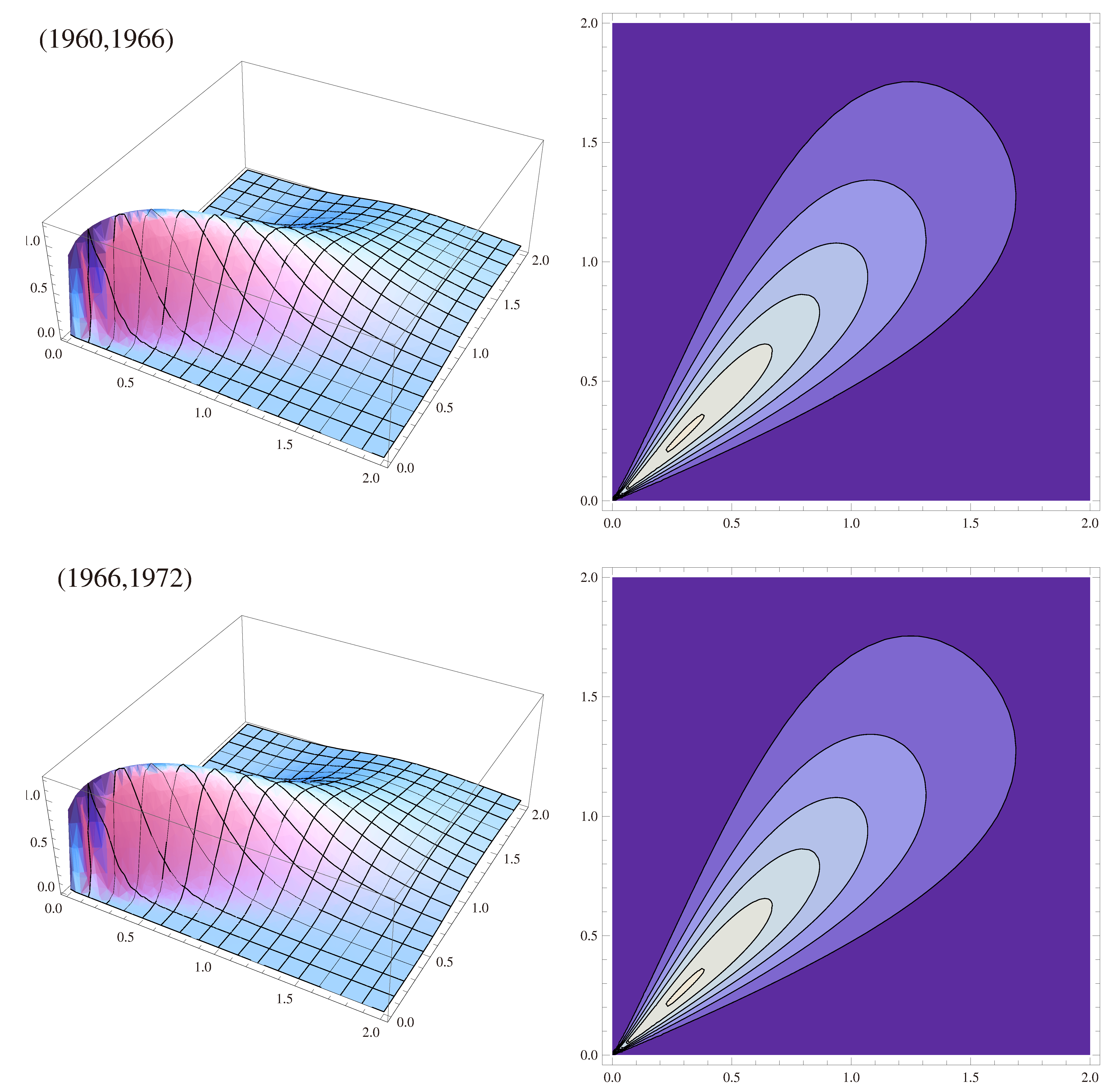
To illustrate the use of the multivariate GB2 distribution to income data, we used the estimated parameters from Singh and Maddala [29], who estimated the income distribution in the US from 1960 to 1972 using data from the US Census Bureau. In Figure 2, we present the joint pdf and the contour plots for the bivariate income Singh–Maddala distribution or the years ( 1960 , 1966 ) in the top panel and years ( 1966 , 1972 ) in the bottom panel. Our estimates suggest that there is a strong positive dependence between income distributions in different years. The contour plots also suggest that such dependence is stronger at the lower tail. The economic interpretation of lower tail dependence is that part of the U.S. citizens experiences serious issues to get out of poverty. More importantly, the shape of the bivariate distribution does not exhibit substantial changes over time, which reflects that the poverty trap has traditionally been a prevalent issue in the US economy, which, according to recent studies, has not been addressed yet [57].
The main contribution of our models to the area of income distribution dynamics is that we can understand non-linear dependencies in bivariate comparisons. This is clearly seen in Figure 2 and the corresponding contour plots. The sort of relationship between the income of a family in 1960 and that in 1966 is much higher in low levels than it is in high levels of income. This result cannot be obtained with a univariate analysis, where each year is analyzed separately from the next. In the bivariate analysis, we have a duplicate of each family in two different years, and so we can assess the dispersion of family trajectories regarding their income level.

6.2. Modeling Compound Precipitation and Wind Events

A key point, for estimating risks associated with climate events, is to build powerful statistical models for modeling compound events. In this section, we show that a multivariate GB2 distribution with q fixed, defined by the expression (10) and with joint probability density function (pdf) given by the expression (11), can be useful for modeling simultaneous precipitation and wind events in the whole range.
The concurrence of precipitation and winds cause significant impacts in our lives. Those impacts can be either negative or positive. For example, extreme precipitation and strong winds happening at the same time can cause major infrastructural damage [58]; however, moderate levels of rain intensity and wind speed can reduce air pollution [59]. This makes it necessary to model not only the right tail of the bivariate distribution but also the rest of it.

6.2.1. Data

For this study, we used the EartH2Observe (E2OBS), WFDEI and ERA-Interim data Merged and Bias-corrected for ISIMIP (EWEMBI) data base [60,61], a global climate dataset freely available on Potsdam Institute for Climate Impact Research website [62], that cover the entire globe, at daily temporal resolution from 1979 to 2016, and 0 . 5 horizontal resolution.
We analyzed two climate variables: precipitation and near-surface wind speed, whose short names in the dataset are p r and s f c W i n d , and that are expressed in kg·m 2 ·s 1 and m·s 1 , respectively. For that, we used as lower thresholds: 0.1/86,400 kg·m 2 ·s 1 (0.1 mm·d 1 ) for precipitation and 0.01 m·s 1 for wind speed (see [63]).
For illustration purposes, we selected four well-known locations at different points of the planet: Alhambra, Granada, Spain; Sagrada Familia, Barcelona, Spain; Statue of Liberty, New York City, United States; and Taipei World Financial Center, Taipei, Taiwan. Then, for each of those locations, we took their nearest point in our 0 . 5 horizontal grid (not considering the points located on the sea, as was the case in Barcelona and Taipei). Finally, we analyzed the bivariate truncated distribution of precipitation and near-surface wind speed in each of those near locations in the last decade, from 1 January 2007 to 31 December 2016 at daily temporal resolution.
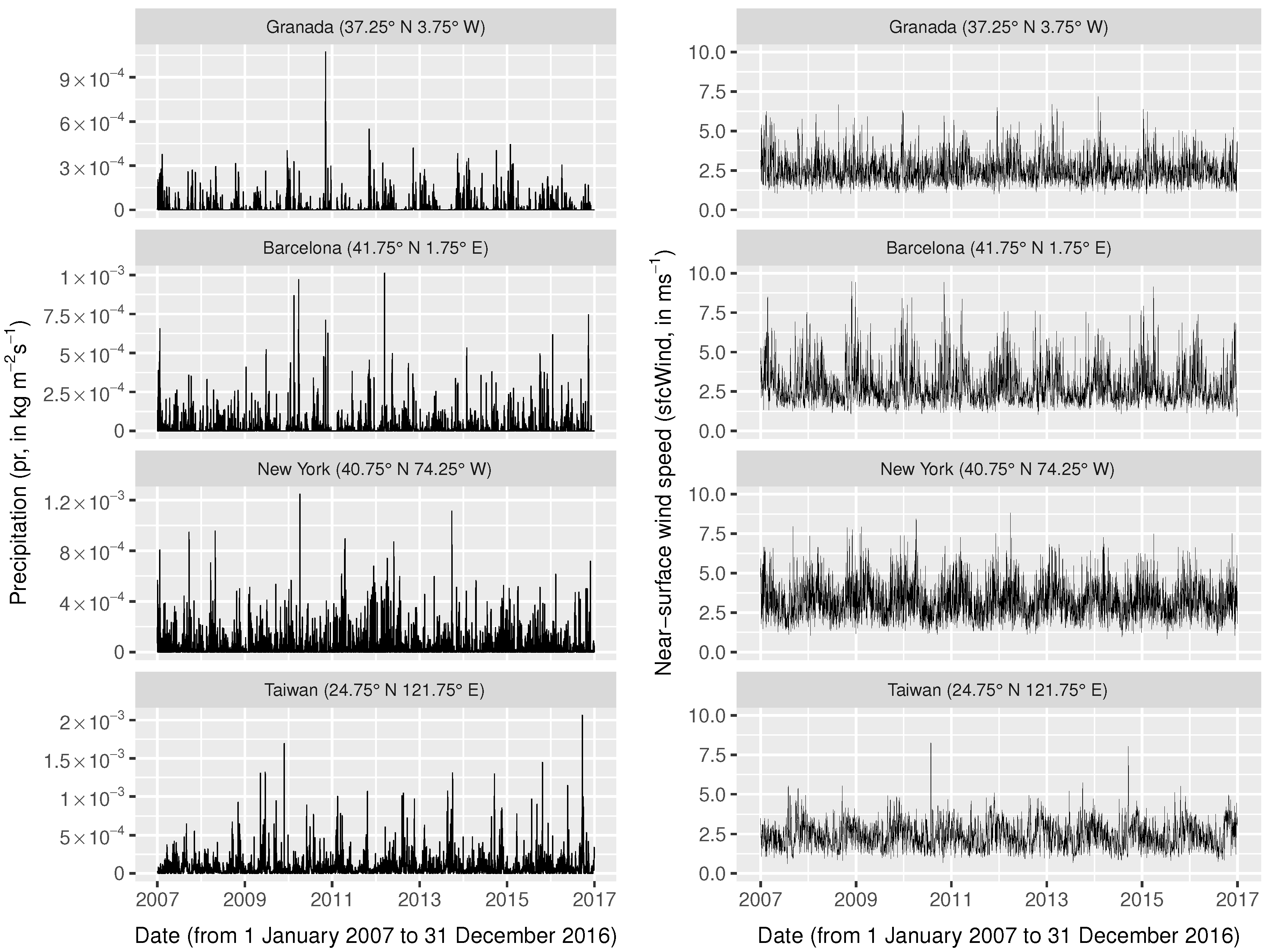
Table 1 provides a list of those selected locations and their coordinates, the coordinates of the grid points chosen in our dataset from those locations, and the probability of compound event (proportion of days with simultaneous positive values, over the thresholds, of both variables, in the period considered, in a particular grid point). Figure 3 shows the daily time series of both variables ( p r and s f c W i n d ) for the four grid points chosen.

6.2.2. Methods

We fitted a bivariate GB2 (with q fixed) model, described in Section 3.2, with unknown parameter vector θ = ( q 0 , p 1 , p 2 , a 1 , a 2 , σ 1 , σ 2 ) and joint pdf given by the expression (11), to each of the four bivariate truncated dataset (corresponding to the days with simultaneous positive values of both variables, in the whole range, from 1 January 2007 to 31 December 2016, by maximum likelihood method.
The corresponding log-likelihood function, from the expression (11), can be expressed as follows
log ( θ ) = j = 1 N log f ( z 1 j , z 2 j | θ ) = N { log [ Γ ( q 0 + p 1 + p 2 ) ] log [ Γ ( q 0 ) ] log [ Γ ( p 1 ) ] log [ Γ ( p 2 ) ] } + N { log [ a 1 ] + log [ a 2 ] log [ σ 1 ] log [ σ 2 ] } + ( a 1 p 1 1 ) j = 1 N log ( z 1 j / σ 1 ) + ( a 2 p 2 1 ) j = 1 N log ( z 2 j / σ 2 ) + ( q 0 + p 1 + p 2 ) j = 1 N log [ 1 + ( z 1 j / σ 1 ) a 1 + ( z 2 j / σ 2 ) a 2 ]
where ( z 1 j , z 2 j ) , j = 1 , , N is a sample of bivariate data, f ( z 1 j , z 2 j | θ ) is its joint pdf, N is the sample size, and the maximum likelihood estimation of the parameter vector θ ^ is the one that maximizes log ( θ ) .
Maximum likelihood estimates of the parameters θ were computed by using the R software function optimx, with the limited memory quasi-Newton L-BFGS-B algorithm, considering the p r variable expressed in 10 4 kg·m 2 ·s 1 and the s f c W i n d variable expressed in m·s 1 . We also calculated the value of the Akaike information criterion ( A I C ), given by following expression [64]
A I C = 2 log ( θ ^ ) + 2 K ,
where K is the number of parameters of the model and a lower A I C value indicates a better fit, which could be used in future work as a goodness-of-fit measure to compare with alternative bivariate models. As a final remark, it can be noted that the simulation of multivariate GB2 distribution with q fixed (defined by expression 10) can be done in the following way: first, we choose the shape and scale parameters σ i , a i , p i , i = 1 , 2 , , m and q 0 ; then, we simulate a sample of size m of independent Gamma random variables X 1 , , X m and a single Gamma variable Y 0 with shape parameter q 0 , independent of previous sample; finally, we construct the vector Z 1 , , Z m according to definition (10)-this methodology can be extended easily to the rest of multivariate GB2 distributions defined in the paper.

6.2.3. Results

Table 2 shows the parameter estimates and the values of A I C statistic obtained from the bivariate GB2 (with q fixed) model to the four truncated datasets by maximum likelihood (standard errors in parenthesis). It can be noted that all the parameter estimates are statistically significant at a 0.05 level of significance, assuming the asymptotic normality of the maximum likelihood estimates.
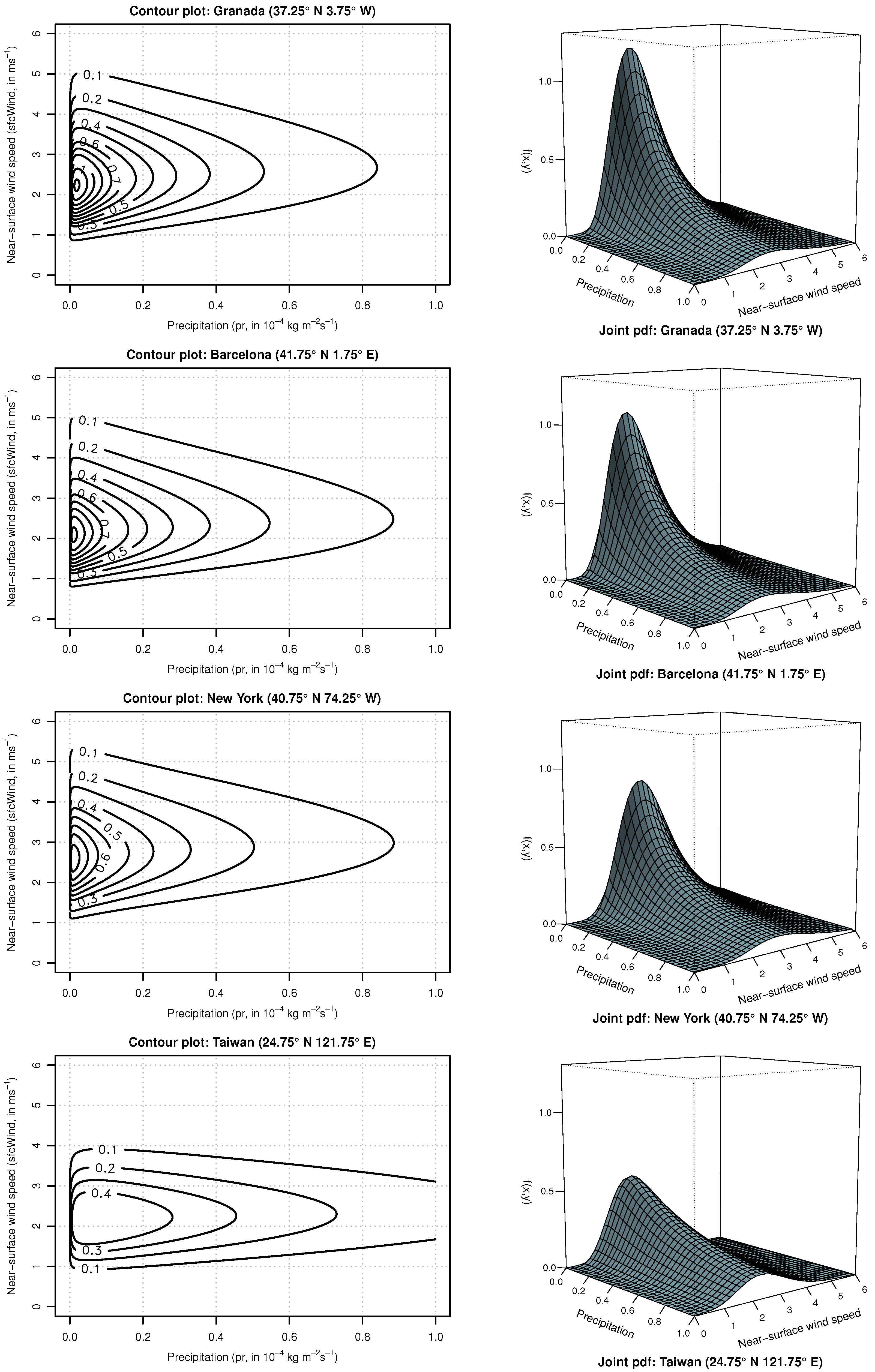
Finally, Figure 4 shows the contour plots and joint pdfs of the bivariate GB2 distribution with q fixed, in which we can see the existing relation between precipitation and near-surface wind speed, in the four locations analyzed. The different shapes they take can be noted, all positively skewed, and with a mode very close to the threshold in the case of p r variable and within 2–3 m·s 1 in the case of s f c W i n d variable.
Economic and practical results follow from the analysis of high-frequency rain and wind data. Firstly, we may characterize the four locations in terms of the risk of large rain or wind measurements. These characterizations are important to insurers. Insurance companies cover weather events, but they try to diversify their exposure to risk. When looking at the raw data in Figure 3, it is difficult to observe an explicit dependence between the two series of rain and wind measurements, besides the relative level in every location. The dependence between the two components does not arise naturally. After our analysis, we conclude that, by obtaining a dependence structure through our models, we can identify features that are relevant for insurers. Insurance companies seek to cover uncorrelated risks. In our analysis, insurers would discard one risk rather than the location in order not to accumulate too much exposure, due to the existence of dependence between the two phenomena. In those cases, reinsurers or consortiums of insurers would cover the rest. We can also confirm that some locations such as Taiwan have stronger tail dependence than others.

7. Conclusions and Future Research

In this paper, we propose several multivariate classes of GB2 distributions. The first class is based on stochastic dependent representations defined in terms of gamma random variables. Then, a general class of multivariate GB2 distributions is introduced where all the marginal distributions are GB2 with all the shape and scale parameters are different. The second class is based on a generalization of the distribution of order statistics. This construction results in a multivariate GB2 distribution with support above the diagonal. We discuss two important applications of these distributions: the modeling of bivariate income distributions and the modeling of compound precipitation and wind events over the entire range.
Future research can be developed in several directions. By means of monotonic transformations of the marginal distributions, models with support in R n can be obtained, which can be useful to model data of returns of dependent financial assets. On the other hand, joint modeling of dependent risks can be another active field of research, together with the computation of multivariate risk dependence measures (see [65,66,67]).

Author Contributions

The authors contributed equally to this work. All authors have read and agreed to the published version of the manuscript.

Funding

The authors acknowledge partial financial support from the Ministerio de Ciencia e Innovación Projects PID2019-105986GB-C21 (M.G.) and PID2019-105986GB-C22 (J.M.S., V.J., F.P.).

Acknowledgments

F.P. acknowledges the European COST Action DAMOCLES (CA17109) for stimulating research in climate compound events. The authors are grateful for the constructive suggestions provided by the reviewers, which improved the paper.

Conflicts of Interest

The authors declare no conflict of interest. The funders had no role in the design of the study; in the collection, analyses, or interpretation of data; in the writing of the manuscript, or in the decision to publish the results.

Appendix A. Some Results about Whittaker’s and Hypergeometric Functions

The Whittaker function W λ , μ ( z ) is a solution of the equation,
d 2 W d z 2 + 1 4 + λ z + 1 4 μ 2 z 2 W = 0 .
Details about the Whittaker function can be found in ([68], sections 9.22 and 9.23). The Whittaker function admits the integral representation,
W λ , μ ( z ) = z λ e z / 2 Γ ( μ λ + 2 2 ) 0 t μ λ 1 / 2 e t 1 + t z μ + λ 1 / 2 d t ,
where R e ( μ λ ) > 1 / 2 , | a r g z | < π . We have next the result about the integral of the Whittaker function (see [68], formula 7.621.3),
0 e s t t α W λ , μ ( q t ) d t = = Γ ( α + μ + 3 2 ) Γ ( α μ + 3 2 ) q μ + 1 2 Γ ( α λ 2 ) s + q 2 α μ 3 2 × × F α + μ + 3 2 , μ λ + 1 2 ; α λ + 2 ; 2 s q 2 s + q ,
with R e ( α ± μ + 3 2 ) > 0 , R e ( s ) > q 2 , q > 0 , and F ( , ; ; ) is the Gauss hypergeometric function (e.g., [68], section 9.1).
On the other hand, we have
0 1 ( 1 x ) μ 1 x ν 1 p F q ( a 1 , , a p ; b 1 , , b q ; a x ) d x = = Γ ( μ ) Γ ( ν ) Γ ( μ + ν ) p + 1 F q + 1 ( ν , a 1 , , a p ; μ + ν , b 1 , , b q ; a )
with R e μ > 0 , R e ν > 0 , p q + 1 , if p = q + 1 , then | a | < 1 (see [68], section 7.5)

References

  1. Cowell, F.A. Measurement of Inequality. In Handbook of Income Distribution; Atkinson, A.B., Bourguignon, F., Eds.; Elsevier: Amsterdam, The Netherlands, 2000; Volume 1, pp. 87–166. [Google Scholar]
  2. Slottje, D.J. Using grouped data for constructing inequality indices: Parametric vs. non-parametric methods. Econ. Lett. 1990, 32, 193–197. [Google Scholar] [CrossRef]
  3. Parker, S.C. The generalized beta as a model for the distribution of earnings. Econ. Lett. 1999, 62, 197–200. [Google Scholar] [CrossRef]
  4. McDonald, J.B. Some generalized functions for the size distribution of income. Econometrica 1984, 52, 647–663. [Google Scholar] [CrossRef]
  5. Butler, R.J.; McDonald, J.B. Using incomplete moments to measure inequality. J. Econom. 1989, 42, 109–119. [Google Scholar] [CrossRef]
  6. Majumder, A.; Chakravarty, S.R. Distribution of Personal Income: Development of a New Model and Its Application to U.S. Income Data. J. Appl. Econom. 1990, 5, 189–196. [Google Scholar] [CrossRef]
  7. McDonald, J.B.; Xu, Y.J. A generalization of the beta distribution with applications. J. Econom. 1995, 66, 133–152. [Google Scholar] [CrossRef]
  8. Chotikapanich, D.; Prasada Rao, D.S.; Tang, K.K. Estimating Income Inequality in China Using Grouped Data and the Generalized Beta Distribution. Rev. Income Wealth 2007, 53, 127–147. [Google Scholar] [CrossRef]
  9. Kleiber, C. On the Lorenz order within parametric families of income distributions. Sankhya B 1999, 61, 514–517. [Google Scholar]
  10. Sarabia, J.M.; Castillo, E.; Slottje, D.J. Lorenz ordering between McDonald’s generalized functions of the income size distribution. Econ. Lett. 2002, 75, 265–270. [Google Scholar] [CrossRef]
  11. McDonald, J.B.; Butler, R.J. Some generalized mixture distributions with an application to unemployment duration. In The Review of Economics and Statistics; MIT Press: Cambridge, MA, USA, 1987; pp. 232–240. [Google Scholar]
  12. McDonald, J.B.; Butler, R.J. Regression models for positive random variables. J. Econom. 1990, 43, 227–251. [Google Scholar] [CrossRef]
  13. Cummins, J.D.; Dionne, G.; McDonald, J.B.; Pritchett, B.M. Applications of the GB2 family of distributions in modeling insurance loss processes. Insur. Math. Econ. 1990, 9, 257–272. [Google Scholar] [CrossRef] [Green Version]
  14. Dutta, K.K.; Babbel, D.F. Extracting Probabilistic Information from the Prices of Interest Rate Options: Tests of Distributional Assumptions. J. Bus. 2005, 78, 841–870. [Google Scholar] [CrossRef]
  15. Kmietowicz, Z.W. The Bivariate Lognormal Model for the Distribution of Household Size and Income. Manch. Sch. Econ. Soc. Stud. 1984, 52, 196–210. [Google Scholar] [CrossRef]
  16. Nalbach-Leniewska, A. Measures of Dependence of the Multivariate Lognormal Distribution. Math. Oper.-Ser. Stat. 1979, 10, 381–387. [Google Scholar] [CrossRef]
  17. Mardia, K.V. Multivariate Pareto distributions. Ann. Math. Stat. 1962, 33, 1008–1015. [Google Scholar] [CrossRef]
  18. Arnold, B.C. Pareto Distributions; International Cooperative Publishing House: Fairland, MD, USA, 1983. [Google Scholar]
  19. Chiragiev, A.; Landsman, Z. Multivariate flexible Pareto model: Dependency structure, properties and characterizations. Stat. Probab. Lett. 2009, 79, 1733–1743. [Google Scholar] [CrossRef]
  20. Asimit, A.V.; Furman, E.; Vernic, R. On a multivariate Pareto distribution. Insur. Math. Econ. 2010, 46, 308–316. [Google Scholar] [CrossRef] [Green Version]
  21. Slottje, D.J. A measure of income inequality based upon the beta distribution of the second kind. Econ. Lett. 1984, 15, 369–375. [Google Scholar] [CrossRef]
  22. Slottje, D.J. Relative price changes and inequality in the size distribution of various components of income. J. Bus. Econ. Stat. 1987, 5, 19–26. [Google Scholar] [CrossRef]
  23. Arnold, B.C.; Castillo, E.; Sarabia, J.M. Conditional Specification of Statistical Models; Springer: New York, NY, USA, 1998. [Google Scholar]
  24. Arnold, B.C.; Castillo, E.; Sarabia, J.M. Conditionally specified distributions: An introduction (with discussion). Stat. Sci. 2001, 16, 249–274. [Google Scholar]
  25. Arnold, B.C. Bivariate distributions with Pareto conditionals. Stat. Probab. Lett. 1987, 5, 263–266. [Google Scholar] [CrossRef]
  26. Arnold, B.C.; Castillo, E.; Sarabia, J.M. Multivariate distributions with generalized Pareto conditionals. Stat. Probab. Lett. 1993, 17, 361–368. [Google Scholar] [CrossRef]
  27. Sarabia, J.M.; Castillo, E.; Pascual, M.; Sarabia, M. Bivariate income distributions with lognormal conditionals. J. Econ. Inequal. 2007, 5, 371–383. [Google Scholar] [CrossRef] [Green Version]
  28. Sarabia, J.M. Multivariate GB2 Distributions. In Proceedings of the 6th St. Petersburg Workshop on Simulation, St. Petersburg, Russia, 28 June–4 July 2009; pp. 237–241. [Google Scholar]
  29. Singh, S.K.; Maddala, G.S. A function for the size distribution of incomes. Econometrica 1976, 44, 963–970. [Google Scholar] [CrossRef]
  30. Dagum, C. A new model of personal income distribution: Specification and estimation. Econ. Appl. 1977, 30, 413–437. [Google Scholar]
  31. Kleiber, C.; Kotz, S. Statistical Size Distributions in Economics and Actuarial Sciences; John Wiley: New York, NY, USA, 2003. [Google Scholar]
  32. Arnold, B.C.; Sarabia, J.M. Majorization and the Lorenz Order with Applications in Applied Mathematics and Economics; Springer: Berlin/Heidelberg, Germany, 2018. [Google Scholar]
  33. Chotikapanich, D.; Griffiths, W.E.; Hajargasht, G.; Karunarathne, W.; Prasada Rao, D.S. Using the GB2 Income Distribution. Econometrics 2018, 6, 21. [Google Scholar] [CrossRef] [Green Version]
  34. Jones, M.C. Families of distributions arising from distributions of order statistics (with discussion). Test 2004, 13, 1–43. [Google Scholar] [CrossRef]
  35. Rada-Mora, E.A.; Nagar, D. Multivariate generalized beta distribution. Random Oper. Stoch. Equ. 2007, 15, 163–180. [Google Scholar] [CrossRef]
  36. Yang, X.; Frees, E.W.; Zhang, Z. A generalized beta copula with applications in modeling multivariate long-tailed data. Insur. Math. Econ. 2011, 49, 265–284. [Google Scholar] [CrossRef]
  37. Sarabia, J.M.; Prieto, F.; Jorda, V. Bivariate beta-generated distributions with applications to well-being data. J. Stat. Distrib. Appl. 2014, 1, 15. [Google Scholar] [CrossRef] [Green Version]
  38. Cockriel, W.M.; McDonald, J.B. Two multivariate generalized beta families. Commun. Stat.-Theory Methods 2018, 47, 5688–5701. [Google Scholar] [CrossRef]
  39. Balakrishnan, N.; Lai, C.D. Continuous Bivariate Distributions, 2nd ed.; Springer: New York, NY, USA, 2009. [Google Scholar]
  40. Olkin, I.; Liu, R. A bivariate beta distribution. Stat. Probab. Lett. 2003, 62, 407–412. [Google Scholar] [CrossRef]
  41. Fang, K.T.; Kotz, S.; Ng, K.W. Symmetric Multivariate and Related Distributions; Chapman and Hall: London, UK, 1990. [Google Scholar]
  42. Jones, M.C. A dependent bivariate t distribution with marginals on different degrees of freedom. Stat. Probab. Lett. 2002, 56, 163–170. [Google Scholar] [CrossRef]
  43. Sarhan, A.M.; Balakrishnan, N. A new class of bivariate distributions and its mixture. J. Multivar. Anal. 2007, 98, 1508–1527. [Google Scholar] [CrossRef] [Green Version]
  44. El-Bassiouny, A.H.; Jones, M.C. A bivariate F distribution with marginals on arbitrary numerator and denominator degrees of freedom, and related bivariate beta and t distributions. Stat. Methods Appl. 2009, 18, 465–481. [Google Scholar] [CrossRef] [Green Version]
  45. Sarabia, J.M.; Gómez-Déniz, E. Construction of multivariate distributions: A review of some recent results (with discussion). Stat. Oper. Res. Trans. 2008, 32, 3–36. [Google Scholar]
  46. Esary, J.D.; Proschan, F.; Walkup, D.W. Association of random variables, with applications. Ann. Math. Stat. 1967, 38, 1466–1474. [Google Scholar] [CrossRef]
  47. Guillén, M.; Sarabia, J.M.; Prieto, F. Simple risk measure calculations for sums of positive random variables. Insur. Math. Econ. 2013, 51, 273–280. [Google Scholar] [CrossRef]
  48. Kleiber, C. Dagum vs. Singh-Maddala income distributions. Econ. Lett. 1996, 53, 265–268. [Google Scholar] [CrossRef]
  49. Jones, M.C.; Larsen, P.V. Multivariate distributions with support above the diagonal. Biometrika 2004, 91, 975–986. [Google Scholar] [CrossRef]
  50. Vinh, A.; Griffiths, W.E.; Chotikapanich, D. Bivariate income distributions for assessing inequality and poverty under dependent samples. Econ. Model. 2010, 27, 1473–1483. [Google Scholar] [CrossRef] [Green Version]
  51. Takahasi, K. Note on the Multivariate Burr’s Distribution. Ann. Inst. Stat. Math. 1965, 17, 257–260. [Google Scholar] [CrossRef]
  52. Björklund, A.; Jäntti, M. Intergenerational Income Mobility in Sweden Compared to the United States. Am. Econ. Rev. 1997, 87, 1009–1018. [Google Scholar]
  53. Chetty, R.; Hendren, N.; Kline, P.; Saez, E.; Turner, N. Is the United States still a land of opportunity? Recent trends in intergenerational mobility. Am. Econ. Rev. 2014, 104, 141–147. [Google Scholar] [CrossRef] [Green Version]
  54. Greenwood, J.; Guner, N.; Kocharkov, G.; Santos, C. Marry your like: Assortative mating and income inequality. Am. Econ. Rev. 2014, 104, 348–353. [Google Scholar] [CrossRef] [Green Version]
  55. Maasoumi, E.; Wang, L. The gender gap between earnings distributions. J. Political Econ. 2019, 127, 2438–2504. [Google Scholar] [CrossRef] [Green Version]
  56. Jäntti, M.; Sierminska, E.M.; Van Kerm, P. Modeling the Joint Distribution of Income and Wealth. Res. Econ. Inequal. 2015, 23, 301–327. [Google Scholar]
  57. Chetty, R.; Hendren, N. The impacts of neighborhoods on intergenerational mobility I: Childhood exposure effects. Q. J. Econ. 2018, 133, 1107–1162. [Google Scholar] [CrossRef]
  58. Martius, O.; Pfahl, S.; Chevalier, C. A global quantification of compound precipitation and wind extremes. Geophys. Res. Lett. 2016, 43, 7709–7717. [Google Scholar] [CrossRef] [Green Version]
  59. Cugerone, K.; De Michele, C.; Ghezzi, A.; Gianelle, V. Aerosol removal due to precipitation and wind forcings in Milan urban area. J. Hydrol. 2018, 556, 1256–1262. [Google Scholar] [CrossRef]
  60. Frieler, K.; Lange, S.; Piontek, F.; Reyer, C.P.; Schewe, J.; Warszawski, L.; Zhao, F.; Chini, L.; Denvil, S.; Emanuel, K.; et al. Assessing the impacts of 1.5 °C global warming-simulation protocol of the Inter-Sectoral Impact Model Intercomparison Project (ISIMIP2b). In Geoscientific Model Development; Copernicus Publications: Argentina, Germany, 2017. [Google Scholar]
  61. Lange, S. Bias correction of surface downwelling longwave and shortwave radiation for the EWEMBI dataset. Earth Syst. Dyn. 2018, 9, 627–645. [Google Scholar] [CrossRef] [Green Version]
  62. Lange, S. EartH2Observe, WFDEI and ERA-Interim Data Merged and Bias-Corrected for ISIMIP (EWEMBI). V. 1.1. GFZ Data Services. 2019. Available online: https://doi.org/10.5880/pik.2019.004 (accessed on 23 October 2020).
  63. Lange, S. Trend-preserving bias adjustment and statistical downscaling with ISIMIP3BASD (v1. 0). In Geoscientific Model Development; Copernicus Publications: Argentina, Germany, 2019; Volume 2. [Google Scholar]
  64. Akaike, H. A new look at the statistical model identification. IEEE Trans. Autom. Control 1974, 19, 716–723. [Google Scholar] [CrossRef]
  65. Guillén, M.; Sarabia, J.M.; Belles-Sampera, J.; Prieto, F. Distortion risk measures for nonnegative multivariate risks. J. Oper. Risk 2018, 13, 35–57. [Google Scholar] [CrossRef]
  66. Roozegar, R.; Balakrishnan, N.; Jamalizadeh, A. On moments of doubly truncated multivariate normal mean-variance mixture distributions with application to multivariate tail conditional expectation. J. Multivar. Anal. 2020, 177, 104586. [Google Scholar] [CrossRef]
  67. Sarabia, J.M.; Guillén, M.; Chuliá, H.; Prieto, F. Tail risk measures using flexible parametric distributions. Stat. Oper. Res. Trans. 2019, 53, 223–236. [Google Scholar]
  68. Gradshteyn, I.S.; Ryzhik, I.M. Table of Integrals, Series, and Products, 5th ed.; Jeffrey, A., Ed.; Academic Press: San Diego, CA, USA, 1994. [Google Scholar]
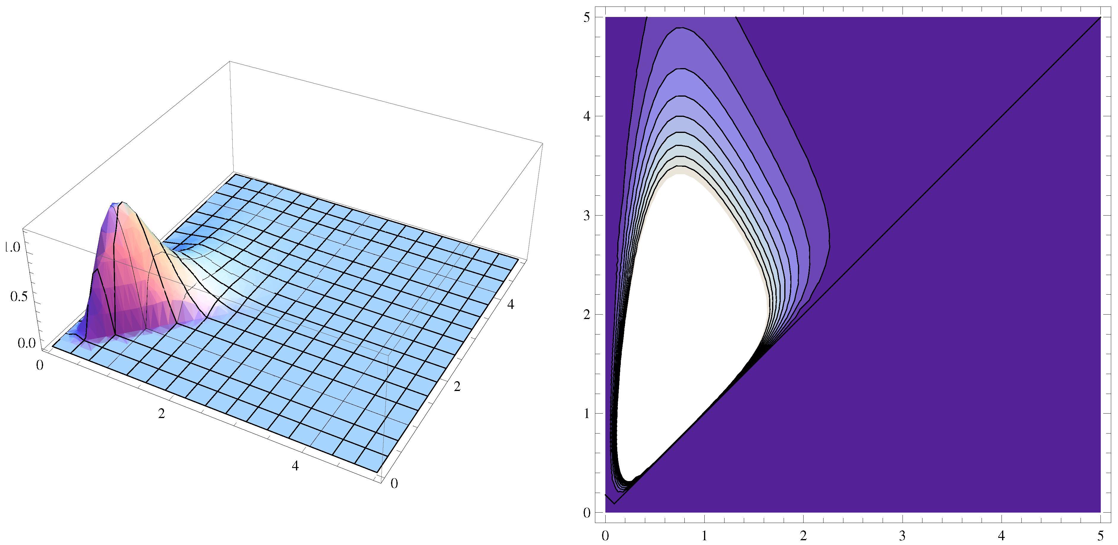
Figure 1. Joint pdf and contour plots of the Bivariate GB2 distributions with support above than diagonal, with σ i = 1 , i = 1 , 2 and p i = 2 , i = 1 , 2 , 3 .
Mathematics 09 00072 g001
Figure 2. Joint pdf and contour plots of the bivariate income Singh–Maddala distribution for the years: ( 1960 , 1966 ) (top); and ( 1966 , 1972 ) (bottom).
Mathematics 09 00072 g002
Figure 3. Daily time series of precipitation ( p r ) and near-surface wind speed ( s f c W i n d ) over four selected grid points (see Table 1), using EWEMBI data, from 1 January 2007 to 31 December 2016.
Mathematics 09 00072 g003
Figure 4. Contour plots and joint pdf of the bivariate GB2 distribution with q fixed, corresponding to the four grid points indicated in Table 1.
Mathematics 09 00072 g004
Table 1. Selected locations, their coordinates, the coordinates of the grid points chosen in our dataset and their probability of compound event (simultaneous precipitation and wind events, over the thresholds of 0.1 mm·d 1 and 0.01 m·s 1 , in the period 2007–2016).
LocationCoordinatesGrid PointProbability of
CoordinatesCompound Event
Alhambra, Granada, Spain 37.17627 N 3.58810 W 37.25 N 3.75 W0.2935
Sagrada Familia, Barcelona, Spain 41.40404 N 2.17443 E 41.75 N 1.75 E0.3452
Statue of Liberty, New York City, USA 40.68944 N 74.04453 W 40.75 N 74.25 W0.4610
Taipei World Financial Center, Taiwan 25.03428 N 121.56450 E 24.75 N 121.75 E0.8555
Table 2. Parameter estimates and A I C statistics, from the bivariate GB2 model with q fixed (Equation (11)), to the four bivariate truncated datasets by maximum likelihood, with standard errors in parenthesis ( p r expressed in 10 4 kg·m 2 ·s 1 and s f c W i n d expressed in m·s 1 ).
Location q ^ 0 p ^ 1 p ^ 2 a ^ 1 a ^ 2 σ ^ 1 σ ^ 2 AIC
Granada16.31873.03697.97990.47021.135512.16075.3893−3992.44
( 37.25 N 3.75 W)(2.8526)(1.0185)(2.4878)(0.0783)(0.1419)(4.0787)(1.2403)
Barcelona16.65112.081011.75000.56270.928016.48143.9937−5004.23
( 41.75 N 1.75 E)(2.1999)(0.4537)(3.1215)(0.0626)(0.0878)(4.0430)(0.9927)
New York13.80622.50096.72160.48621.317916.50385.6226−7793.07
( 40.75 N 74.25 W)(1.8616)(0.5979)(1.3626)(0.0587)(0.1096)(4.0350)(0.8037)
Taiwan11.07102.14982.36240.61202.088911.18615.4784−14,855.81
( 24.75 N 121.75 E)(2.3232)(0.3306)(0.4214)(0.0542)(0.2086)(3.9155)(0.5138)
Publisher’s Note: MDPI stays neutral with regard to jurisdictional claims in published maps and institutional affiliations.