An Approach Integrating Simulated Annealing and Variable Neighborhood Search for the Bidirectional Loop Layout Problem

Abstract

In the bidirectional loop layout problem (BLLP), we are given a set of machines, a set of locations arranged in a loop configuration, and a flow cost matrix. The problem asks to assign machines to locations so as to minimize the sum of the products of the flow costs and distances between machines. The distance between two locations is calculated either in the clockwise or in the counterclockwise direction, whichever path is shorter. We propose a hybrid approach for the BLLP which combines the simulated annealing (SA) technique with the variable neighborhood search (VNS) method. The VNS algorithm uses an innovative local search technique which is based on a fast insertion neighborhood exploration procedure. The computational complexity of this procedure is commensurate with the size of the neighborhood, that is, it performs $O\left(1\right)$ operations per move. Computational results are reported for BLLP instances with up to 300 machines. They show that the SA and VNS hybrid algorithm is superior to both SA and VNS used stand-alone. Additionally, we tested our algorithm on two sets of benchmark tool indexing problem instances. The results demonstrate that our hybrid technique outperforms the harmony search (HS) heuristic which is the state-of-the-art algorithm for this problem. In particular, for the 4 Anjos instances and 4 sko instances, new best solutions were found. The proposed algorithm provided better average solutions than HS for all 24 Anjos and sko instances. It has shown robust performance on these benchmarks. For 20 instances, the best known solution was obtained in more than $50\%$ of the runs. The average time per run was below 10 s. The source code implementing our algorithm is made publicly available as a benchmark for future comparisons.

1. Introduction

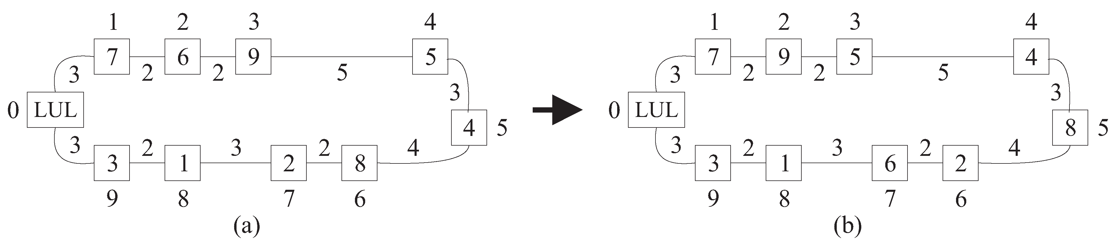
The problem studied in this paper belongs to the family of machine layout problems that can be successfully modeled by representing solutions as permutations of machines to be assigned to a given set of locations. We do not make an assumption that locations are equidistant. As it is typical in loop layout formulations, one of locations is reserved for the Load/Unload (LUL) station. It may be considered as the starting point of the loop. The distance between two locations is calculated either in the clockwise or in the counterclockwise direction, whichever path is the shorter. The objective of the problem is to determine the assignment of machines to locations which minimizes the sum of the products of the material flow costs and distances between machines. In the remainder of this paper, we refer to the described problem as the bidirectional loop layout problem (BLLP for short). An example of loop layout is shown in Figure 1, where machines $M_3$, $M_1$, $M_6$, $M_4$, $M_7$, $M_2$ and $M_5$ are assigned to locations 1, 2, 3, 4, 5, 6 and 7, respectively. The numbers on the edges of the loop indicate distances between adjacent locations. Distance is the length of the shortest route between two locations along the loop.

The BLLP finds application in the design of flexible manufacturing systems (FMS). According to the literature (see, for example, a recent survey by Saravanan and Kumar [1]), the loop layout is one of the most preferred configurations in FMS because of their relatively low investment costs and material handling flexibility. In this layout type, a closed-loop material handling path passes through each machine exactly once. In many cases, the machines are served by an automated guided vehicle (AGV). All materials enter and leave the system at the LUL station. The focus of this paper is on a variation of the loop layout problem where the AGV is allowed to transport the materials bidirectionally along the loop, that is, it can travel either clockwise or counterclockwise, depending on which route is shorter. A related problem, called the unidirectional loop layout problem (ULLP), is obtained by restricting materials to be transported in only one direction around the loop [2].

The model of the bidirectional loop layout can also be applied to other domains such as tool indexing and broadcast scheduling. The tool indexing problem asks to allocate cutting tools to slots (tool pockets) in a tool magazine with the objective of minimizing the tool change time on a CNC (computer numerically controlled) machine. The turret of the CNC machine can rotate in both directions. Frequently, in practice, the number of slots exceeds the number of tools required to accomplish a job. Detailed information on this problem can be found in [3,4,5]. Liberatore [6] considered the bidirectional loop layout problem in the context of broadcast scheduling. In this application, a weighted graph is constructed whose vertices represent server data units and edge weights show the strength of dependencies between consecutive requests for data units. The problem is to arrange the vertices around a circle so as to minimize the sum of weighted distances between all pairs of vertices. In this BLLP instance, the distance between adjacent locations is assumed to be fixed at 1.

In general, an instance of the BLLP is given by the number of machines n, a symmetric $n\times n$ matrix $D=\left(d_{kl}\right)$ with entries representing the distances between locations, and a symmetric $n\times n$ matrix $C=\left(c_{ij}\right)$ whose entry $c_{ij}$ represents the cost of the flow of material between machines i and j. We denote the set of machines as $M=\{0,1,\dots ,n-1\}$. For convenience, we let 0 refer to the LUL station. In the formulation of the problem, it is assumed the LUL station to be in location 0. Let $\mathsf{\Pi }\left(n\right)=\left\{p\right\}$, $p=\left(p\right(0),p(1),\dots ,p(n-1\left)\right)$, be the set of all n-element permutations defined on M such that $p\left(0\right)=0$. Then, mathematically, the BLLP can be expressed as:

$$\underset{p\in \mathsf{\Pi }\left(n\right)}{min}F\left(p\right)=\sum _{k=0}^{n-2}\sum _{l=k+1}^{n-1}{d}_{kl}{c}_{p\left(k\right)p\left(l\right)},$$

(1)

where $p\left(k\right)$ and $p\left(l\right)$ are the machines in locations k and l, respectively, and $d_{kl}$ is the distance between these two locations. As mentioned above, $p\left(0\right)$ is the LUL station.

The BLLP, as defined by Equation (1), is a special case of the quadratic assignment problem (QAP) formulated by Koopmans and Beckmann [7]. A problem, related to the BLLP, is the single-row equidistant facility layout problem (SREFLP), which is a special case of the QAP, too. The feasible solutions of the SREFLP are one-to-one assignments of n facilities to n locations equally spaced along a straight line. Its objective function is of the form as given in Equation (1). Among other areas, the SREFLP arises in the context of designing flexible manufacturing systems [8,9]. In this application, the machines are assigned to locations along a linear material handling track. For this reason, the SREFLP differs noticeably from the BLLP we address in this paper. Yet another related problem is that of arranging manufacturing cells both inside and outside of the loop. It is assumed that the cells are rectangular in shape. In the literature, this type of problem is called a closed loop layout problem [10].

Loop layout problems have attracted much research interest, as evidenced by a recent survey by Saravanan and Kumar [1]. However, most studies in the literature on loop layout have been devoted to developing algorithms for the unidirectional loop layout model. Nearchou [11] proposed a differential evolution (DE) algorithm for solving the ULLP. The experiments were conducted for a set of randomly generated problem instances with up to 100 machines and 30 parts. The results have shown the superiority of the developed DE heuristic to previous approaches, such as genetic and simulated annealing algorithms. It is notable that, for most instances, the DE algorithm found a good solution in a few CPU seconds. Zheng and Teng [12] proposed another DE implementation for the ULLP, called relative position-coded DE. This heuristic performed slightly better than DE in [11]. However, as remarked by Zheng and Teng, DE is prone to trap into local minima when the problem size gets larger. Kumar et al. [13] applied the particle swarm optimization (PSO) technique to the ULLP. Their PSO implementation compared favorably with the DE algorithm presented in [11]. However, the comparison was done only for relatively small size problem instances. Kumar et al. [14] proposed an artificial immune system-based algorithm for the ULLP in a flexible manufacturing system. The experimental results proved that their algorithm is a robust tool for solving this layout problem. The algorithm performed better than previous methods [11,13]. In order to reduce the material handling cost, the authors proposed to use the shortcuts at suitable locations in the layout. Ozcelik and Islier [15] formulated a generalized ULLP in which it is assumed that loading/unloading equipment can potentially be attached to each workstation. They developed a genetic algorithm for solving this problem. Significant improvements against the model with one LUL station were achieved. Boysen et al. [16] addressed synchronization of shipments and passengers in hub terminals. They studied the problem (called circular arrangement) which is very similar to the ULLP. The authors proposed the dynamic programming-based heuristic solution procedures for this problem. However, it is not clear how well these procedures perform on large-scale problem instances. Saravanan and Kumar [17] presented a sheep flock heredity algorithm to solve the ULLP. Computational tests have shown superior performance in comparison to the existing approaches [11,13,14]. The largest ULLP instances used in [17] had 50 machines and 10 or 20 parts. Liu et al. [18] considered a loop layout problem with two independent tandem AGV systems. Both the AGVs run unidirectionally. The authors applied the fuzzy invasive weed optimization technique to solve this problem. The approach is illustrated for the design of a complex AGV system with two workshops and 35 machines. A computational experiment has shown the efficiency of the approach. There are several exact methods for the solution of the ULLP. Öncan and Altınel [19] developed an algorithm based on the dynamic programming (DP) scheme. The algorithm was tested on a set of problem instances with 20 machines. It failed to solve larger instances because of limited memory storage. Boysen et al. [16] proposed another DP-based exact method. Likewise the algorithm in [19], this method was able to solve only small instances. It did not finish within two hours for instances of size 24. Kouvelis and Kim [2] developed a branch-and-bound (B&B) procedure for solving the ULLP. This procedure was used to evaluate the results of several heuristics described in [2]. A different B&B algorithm was proposed by Lee et al. [20]. The algorithm uses a depth first search strategy and exploits certain network flow properties. These innovations helped to increase the efficiency of the algorithm. It produced optimal solutions for problem instances with up to 100 machines. Later, Öncan and Altınel [19] provided an improved B&B algorithm. They experimentally compared their algorithm against the method of Lee et al. [20]. The new B&B implementation outperformed the algorithm of Lee et al. in terms of both number of nodes in the search tree and computation time. Ventura and Rieksts [21] presented an exact method for optimal location of dwell points in an unidirectional loop system. The algorithm is based on dynamic programming and has polynomial time complexity.

Compared to the ULLP, the bidirectional loop layout problem has received less attention in the literature. Manita et al. [22] considered a variant of the BLLP in which machines are required to be placed on a two-dimensional grid. Additionally, proximity constraints between machines are specified. To solve this problem, the authors proposed a heuristic that consists of two stages: loop construction and loop optimization. In the second stage, the algorithm iteratively improves the solution produced in the first stage. At each iteration, it randomly selects a machine and tries to exchange it either with an adjacent machine or with each of the remaining machines. Rezapour et al. [23] presented a simulated annealing (SA) algorithm for a version of the BLLP in which the distances between machines in the layout are machine dependent. The search operator in this SA implementation relies on the pairwise interchange strategy. The authors have incorporated their SA algorithm into a method for design of tandem AGV systems. Bozer and Rim [24] developed a branch-and-bound algorithm for solving the BLLP. To compute a lower bound on the objective function value, they proposed to use the generalized linear ordering problem and resorted to a fast dynamic programming method to solve it. The algorithm was tested on BLLP instances of size up to 12 facilities. Liberatore [6] presented an $O(logn)$-approximation algorithm for a version of the BLLP in which the distance between each pair of adjacent locations is equal to 1. A simple algorithm with better approximation ratio was provided by Naor and Schwartz [25]. Their algorithm achieves an approximation of $O(\sqrt{logn}loglogn)$. The studies just mentioned have focused either on some modifications of the BLLP or on the exact or approximation methods. We are unaware of any published work that deals with metaheuristic algorithms for the bidirectional loop layout problem in the general case (as shown in Equation (1)).

Another thread of research on bidirectional loop layout is concerned with developing methods for solving the tool indexing problem (TIP). This problem can be regarded as a special case of the BLLP in which the locations (slots) are spaced evenly on a circle and their number may be greater than the number of tools. In the literature, several metaheuristic-based approaches have been proposed for the TIP. Dereli and Filiz [3] presented a genetic algorithm (GA) for the minimization of total tool indexing time. Ghosh [26] suggested a different GA for the TIP. This GA implementation was shown to achieve better performance than the genetic algorithm of Dereli and Filiz. Ghosh [4] has also proposed a tabu search algorithm for the problem. His algorithm uses an exchange neighborhood which is explored by performing pairwise exchanges of tools. Recently, Atta et al. [5] presented a harmony search (HS) algorithm for the TIP. In order to speed up convergence, their algorithm takes advantage of a harmony refinement strategy. The algorithm was tested on problem instances of size up to 100. The results demonstrate its superiority over previous methods (see Tables 4 and 5 in [5]). Thus, HS can be considered as the best algorithm presented so far in the literature for solving the TIP. There is also a variant of the TIP where duplications of tools are allowed. Several authors, including Baykasoğlu and Dereli [27], and Baykasoğlu and Ozsoydan [28,29], contributed to the study of this TIP model.

Various approaches have been proposed for solving facility layout problems that bear some similarity with the BLLP. A fast simulated annealing algorithm for the SREFLP was presented in [30]. Small to medium size instances of this problem can be solved exactly using algorithms provided in [31,32]. Exact solution methods for multi-row facility layout were developed in [33]. The most successful approaches for the earlier-mentioned closed loop layout problem include [10,34,35]. It can be seen from the literature that the most frequently used techniques for solving facility layout problems are metaheuristic-based algorithms. The application of metaheuristics to these problems is summarized in [36] (see Table 1 therein). For a recent classification of facility layout problems, the reader is referred to Hosseini-Nasab et al. [37].

In the conclusions section of the survey paper on loop layout problems, Saravanan and Kumar [1] discuss several research directions that are worth exploring. Among them, the need for developing algorithms for the bidirectional loop layout problem is pointed out. The model of the BLLP is particularly apt in situations where the flow matrix is dense [20]. However, as noted above, the existing computational methods for the general BLLP case are either exact or approximation algorithms. There is a lack of metaheuristic-based approaches for this problem. Several such algorithms, including HS, have been proposed for solving the tool indexing problem, which is a special case of the BLLP. However, the best of these algorithms, i.e. HS, is not the most efficient, especially for larger scale TIP instances. 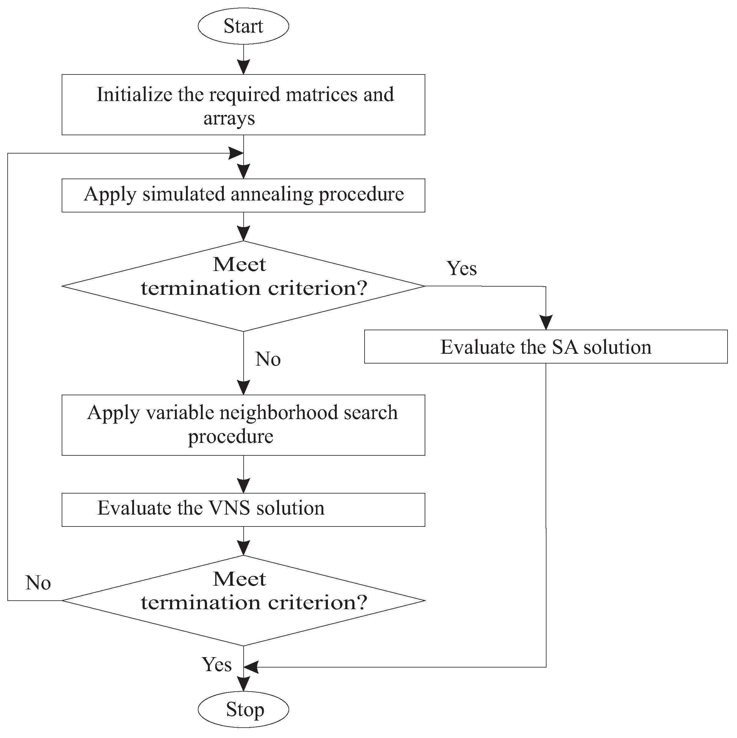In particular, the gaps between the best and average solution values are a little high in many cases (see [5] or Section 5.5). Considering these observations, our motivation is to investigate and implement new strategies to create metaheuristic-based algorithms for the bidirectional loop layout problem. The purpose of this paper is two-fold. First, the paper intends to fill a research gap in the literature by developing a metaheuristic approach for the BLLP. Second, we aim that our algorithm will also be efficient for solving the tool indexing problem. Our specific goal is to improve the results obtained by the HS algorithm. We propose an integrated hybrid approach combining simulated annealing technique and variable neighborhood search (VNS) method. Such a combination has been seen to give good results for a couple of other permutation-based optimization problems, namely, the profile minimization problem [38] and the bipartite graph crossing minimization problem [39]. The crux of the approach is to apply SA and VNS repeatedly. The idea is to let SA start each iteration and then proceed with the VNS algorithm. The latter recursively explores the neighborhood of the solution delivered by SA. Such a strategy allows reducing the execution time of VNS because the solution found by SA is likely to be of good quality. The core of VNS is a local search (LS) procedure. We embed two LS procedures in the VNS framework. One of them relies on performing pairwise interchanges of machines. It is a traditional technique used in algorithms for the QAP. Another LS procedure involves the use of machine insertion moves. In each iteration of this procedure, the entire insertion neighborhood is explored in $O\left(n^2\right)$ time. Thus, the procedure performs only $O\left(1\right)$ operations per move, so it is very efficient. Both move types, pairwise interchanges of machines and insertions, are also used in our implementation of SA for the BLLP. We present computational results comparing the SA and VNS hybrid against these algorithms applied individually. We tested our hybrid algorithm on two sets of BLLP instances and, in addition, on two sets of TIP instances.

The remainder of the paper is organized as follows. In the next section, we show how SA and VNS are integrated to solve the BLLP. Our SA and VNS algorithms are presented in two further sections. Section 5 is devoted to an experimental analysis and comparisons of algorithms. A discussion is conducted in Section 6 and concluding remarks are given in Section 7.

2. Integrating SA and VNS

The basic idea of the VNS method is to systematically explore the neighborhood of the currently best found solution (see, for example, [40]). If initially this solution is of low quality, VNS may require a significant amount of time to get closer to the optimum. Our idea is to speed up this process by starting VNS with a solution generated by another heuristic. We implement this strategy by combining VNS with the SA algorithm. These two techniques are applied in an iterative manner during the search process. A flowchart of the SA and VNS hybrid is shown in Figure 2. Our implementation of this hybrid is equipped with a stopping criterion, where the search is terminated when the maximum time limit, $t_{\lim }$, is reached. Of course, other termination conditions can also be applied depending on different demands. For example, the number of calls to SA and VNS can be specified. In this case, the description of the algorithm is essentially the same as that given below with only minor modifications.

The pseudo-code of the main procedure of the SA and VNS hybrid, denoted as SA-VNS, is given in Algorithm 1. The procedure starts with constructing several matrices and arrays to be used in subsequent calculations. The entry $d_{kl}^{+}$ of the matrix $D^{+}=\left(d_{kl}^{+}\right)$ stands for the clockwise distance between machine locations k and l. Similarly, the matrix $D^{-}=\left(d_{kl}^{-}\right)$ represents distances between locations in the counterclockwise direction. Clearly, $d_{kl}^{-}=d_{lk}^{+}$. The corresponding entry of the matrix D is $d_{kl}=min(d_{kl}^{-},d_{kl}^{+})$. The arrays $a=(a_0,\dots ,a_{n-1})$, $\lambda =({\lambda }_0,\dots ,{\lambda }_{n-1})$ and $\eta =({\eta }_0,\dots ,{\eta }_{n-1})$ are constructed as follows. Let $K=\{0,1,\dots ,n-1\}$ denote the set of machine locations. For each $k\in K$, we find the largest natural number i such that $d_{kl}^{+}⩽d_{kl}^{-}$, where $l=(k+i)(modn)$. Then $a_k=l$ and ${\lambda }_k=i$. If the above inequality is, in fact, an equality, then ${\eta }_k$ is set to 1; otherwise ${\eta }_k$ is set to 0. For example, in Figure 1, $a_4=7$, ${\lambda }_4=3$, ${\eta }_4=0$, $a_5=1$, ${\lambda }_5=4$, and ${\eta }_5=1$. The matrices and arrays constructed in line 1 of Algorithm 1 are left untouched during the execution of SA-VNS. These data are used by both SA and VNS components of the approach. The computational complexity of the initialization step of SA-VNS is $O\left(n^2\right)$.

The algorithm maintains two solutions $\widehat{p}$ and $p^{*}$. The solution $\widehat{p}$ with value $\widehat{f}$ is the best one found in an iteration of SA-VNS (single execution of the “while” loop 3–12 of Algorithm 1). The global best solution over all iterations is denoted as $p^{*}$ and its value as $f^{*}$. Each iteration starts with a call to the SA algorithm. After executing SA for the first time, the maximum time limit on a run of VNS (denoted as $t_{\mathrm{run}\_\mathrm{VNS}}$) is computed. At the initialization phase of SA-VNS, the specified cut-off time $t_{\lim }$ is split between SA time $t_{\lim \_\mathrm{SA}}=\rho t_{\lim }$ and VNS time $t_{\lim \_\mathrm{VNS}}=(1-\rho )t_{\lim }$, where $\rho$ is the preset quota parameter with values between 0 and 1. To compute $t_{\mathrm{run}\_\mathrm{VNS}}$, we use the predicted number of SA-VNS iterations, I, evaluated as $I=\lceil t_{\lim \_\mathrm{SA}}/t_{\mathrm{elapsed}\_\mathrm{SA}}\rceil$, where $t_{\mathrm{elapsed}\_\mathrm{SA}}$ is the time spent by SA in the first iteration. We simply set $t_{\mathrm{run}\_\mathrm{VNS}}=t_{\lim \_\mathrm{VNS}}/I$. The iterative process is stopped when the deadline $t_{\lim }$ is reached while executing either SA (line 8) or VNS (line 13). If, after termination of SA, a running time reserve is available, then the VNS algorithm is triggered. It starts the search from the solution $\widehat{p}$ returned by the SA component of the approach. An iteration of SA-VNS ends with an attempt to improve the global best solution $p^{*}$ (line 11 of Algorithm 1).

Algorithm 1 Integrating simulated annealing and variable neighborhood search

SA-VNS 1:   Construct matrices $D^{+}$, $D^{-}$, D and arrays a, $\lambda$ and $\eta$ 2:    $f^{*}:=\infty$ 3:   while time limit, $t_{\lim }$, not reached do 4:     Apply SA($\widehat{p},\widehat{f},t_{\lim }$) 5:     if SA was executed for the first time then Compute $t_{\mathrm{run}\_\mathrm{VNS}}$ end if 6:     if elapsed time is more than $t_{\lim }$ then 7:         if $\widehat{f}<f^{*}$ then Assign $\widehat{p}$ to $p^{*}$ and $\widehat{f}$ to $f^{*}$ end if 8:         Stop with the solution $p^{*}$ of value $f^{*}$ 9:     end if 10:      Apply VNS($\widehat{p},\widehat{f},t_{\lim },t_{\mathrm{run}\_\mathrm{VNS}}$) 11:      if $\widehat{f}<f^{*}$ then Assign $\widehat{p}$ to $p^{*}$ and $\widehat{f}$ to $f^{*}$ end if 12:   end while 13:   Stop with the solution $p^{*}$ of value $f^{*}$

3. Simulated Annealing

In this section, we present an implementation of the simulated annealing method for the bidirectional loop layout problem. This method is based on an analogy to the metallurgical process of annealing in thermodynamics which involves initial heating and controlled cooling of a material. The idea to use this analogy to solve combinatorial optimization problems has been efficiently exploited by Kirkpatrick et al. [41] and Černý [42]. To avoid being trapped in a local optimum, the SA method also accepts worsening moves with a certain probability [43]. With F denoting the objective function of the BLLP as given by (1), the acceptance probability can be written as $exp(-\mathsf{\Delta }(p,p^{\prime })/T)$, where $\mathsf{\Delta }(p,p^{\prime })=F\left(p^{\prime }\right)-F\left(p\right)$ is the change in cost, called the move gain, p is the current solution (permutation), $p^{\prime }$ is a permutation in a neighborhood of p, and T is the temperature value. To implement SA for the BLLP, we employ two neighborhood structures. One of them is the insertion neighborhood structure $N_1\left(p\right)$, $p\in \mathsf{\Pi }\left(n\right)$. For $p\in \mathsf{\Pi }\left(n\right)$, the set $N_1\left(p\right)$ consists of all permutations that can be obtained from p by removing a machine from its current position in p and inserting it at a different position. As an alternative, we use the pairwise interchange neighborhood structure $N_2\left(p\right)$, $p\in \mathsf{\Pi }\left(n\right)$, whose member set $N_2\left(p\right)$ comprises of all permutations that can be obtained from p by swapping positions of two machines in the permutation p. To guide the choice of the neighborhood type, a $0-1$ valued parameter, $V_{\mathrm{SA}}$, is introduced. If $V_{\mathrm{SA}}=0$, then the pairwise interchange neighborhood structure is employed in the search process; otherwise the search is based on performing insertion moves.

The pseudo-code of the SA implementation for the BLLP is presented in Algorithm 2. The temperature T is initially set to a high value, $T_{\max }$, which is computed once, that is, when SA is invoked for the first time within the SA-VNS framework. For this, we use the formula $T_{\max }={max}_{p^{\prime }\in N^{\prime }}\left|\mathsf{\Delta }(p,p^{\prime })\right|$, where p is a starting permutation generated in line 1 of Algorithm 2 and $N^{\prime }$ is a set of permutations randomly selected either from the neighborhood $N_1\left(p\right)$ (if $V_{\mathrm{SA}}=1$) or from the neighborhood $N_2\left(p\right)$ (if $V_{\mathrm{SA}}=0$). We fixed the size of $N^{\prime }$ at 5000. The temperature is gradually reduced by a geometric cooling schedule $T:=\alpha T$ (line 27) until the final temperature, denoted by $T_{\min }$, is reached, which is very close to zero. We set $T_{\min }=0.0001$. The value of the cooling factor $\alpha$ usually lies in the interval $[0.9,0.99]$. The list of parameters for SA also includes the number of moves, Q, to be attempted at each temperature level. It is common practice to relate Q linearly to the size of the problem instance. According to literature (see, for example, [44]), a good choice is to set Q to $100n$. If SA is configured to perform insertion moves ($V_{\mathrm{SA}}=1$), then an auxiliary array $B=(b_1,\dots ,b_{n-1})$ is used. Relative to a permutation p, its entry $b_r$ for machine $r\in \{1,\dots ,n-1\}$ represents the total flow cost between r (placed in location k) and ${\lambda }_k$ machines that reside closest to r clockwise. Formally, $b_r={\sum }_{i=k+1}^{k+{\lambda }_k}{c}_{rp\left(i\right(modn\left)\right)}$, where $k=\pi \left(r\right)$ and $\pi$ is the inverse permutation of p, defined as follows: if $p\left(k\right)=r$, then $\pi \left(r\right)=k$. It is clear that the content of the array B depends on the permutation p. The time complexity of constructing B (line 4 of SA) is $O\left(n^2\right)$. In the case of the first call to SA, the array B, if needed ($V_{\mathrm{SA}}=1$), is obtained as a byproduct of computing the temperature $T_{\max }$ (line 3). The main body of the algorithm consists of two nested loops. The inner loop distinguishes between two cases according to the type of moves. If a random interchange move is generated ($V_{\mathrm{SA}}=0$), then the candidate solution, $p(r,s)$, obtained by swapping positions of machines r and s is compared against the current solution p by computing the difference between the corresponding objective function values (line 11). Since only machines r and s change their locations, this can be done in linear time. If $V_{\mathrm{SA}}=1$, then an attempt is made to move machine r to a new location l, both selected at random. The move gain $\mathsf{\Delta }$ is obtained by applying the procedure get_gain. Its parameter $\beta$ stores the new value of $b_r$ which, provided the move is accepted, is later used by the procedure insert (line 21). The outer loop of SA is empowered to abort the search prematurely. This happens when the time limit for the run of SA-VNS is passed (line 26).

Algorithm 2 Simulated annealing

SA($\widehat{p},\widehat{f},t_{\lim }$) // Input to SA includes parameters $\alpha ,Q$ and $T_{\min }$ 1:   Randomly generate a permutation $p\in \mathsf{\Pi }\left(n\right)$ and set $\widehat{p}:=p$ 2:   $\widehat{f}=f:=F\left(p\right)$ 3:   if first call to SA then Compute $T_{\max }$ and $\overline{\tau }=\lfloor (log\left(T_{\min }\right)-log\left(T_{\max }\right))/log\alpha \rfloor$ 4:   else if $V_{\mathrm{SA}}=1$ then Construct array B end if 5:   end if 6:   $T:=T_{\max }$ 7:   for $\tau =1,\dots ,\overline{\tau }$ do 8:       for $i=1,\dots ,Q$ do 9:         if $V_{\mathrm{SA}}=0$ then 10:           Pick two machines $r,s$ at random // Let $p(r,s)$ denote the solution obtained from p by swapping positions of machines r and s 11:          Compute $\mathsf{\Delta }:=F\left(p\right(r,s\left)\right)-F\left(p\right)$ 12:       else 13:         Pick machine r and its new position l at random 14:         $\mathsf{\Delta }$:=get_gain($r,l,p,\beta$) 15:       end if 16:       if $\mathsf{\Delta }⩽0$ or $exp(-\mathsf{\Delta }/T)⩾$ random($0,1$) then 17:         $f:=f+\mathsf{\Delta }$ 18:         if $V_{\mathrm{SA}}=0$ then 19:             Swap positions of machines r and s in p 20:         else 21:             insert($r,l,p,\beta$) 22:         end if 23:         if $f<\widehat{f}$ then Assign p to $\widehat{p}$ and f to $\widehat{f}$ end if 24:       end if 25:     end for 26:     if elapsed time for SA-VNS is more than $t_{\lim }$ then return 27:     $T:=\alpha T$ 28:   end for 29:   return

Before continuing with the description of SA, we elaborate on the computation of the move gain $\mathsf{\Delta }$ in the case of $V_{\mathrm{SA}}=1$. For this, we need additional notations. We denote by $K_k^{+}$, $k\in \{0,1,\dots ,n-1\}$, the set of locations $l\in K=\{0,1,\dots ,n-1\}$ such that $d_{kl}^{+}⩽d_{kl}^{-}$ and define $K_k^{-}=K\backslash (K_k^{+}\cup \left\{k\right\})$. In Figure 3, for example, $K_7^{+}=\{8,9,0,1,2\}$, $K_8^{+}=\{9,0,1,2,3\}$, and $K_8^{-}=\{4,5,6,7\}$. Let us denote the set of machines assigned to locations in $K_k^{+}$ by $M_k^{+}$ and those assigned to locations in $K_k^{-}$ by $M_k^{-}$. We notice that since the machine r is being relocated, $M_k^{+}$ is not necessarily equal to $\{p\left(l\right)\mid l\in K_k^{+}\}$ where p is the permutation for which get_gain procedure is applied and which remains untouched during its execution. A similar remark holds for $M_k^{-}$. In the example shown in Figure 3, $M_8^{+}=\{3,0,7,6,9\}$ initially, that is, for $p=(0,7,6,9,5,4,8,2,1,3)$ (part (a) of Figure 3), and $M_8^{+}=\{3,0,7,9,5\}$ after relocating the machine $r=6$ from position 2 to position 7 (part (b) of Figure 3). For a machine s and $M^{\prime }\subset M$, we denote by $c(s,M^{\prime })$ the total flow cost between s and machines in $M^{\prime }$, that is, $c(s,M^{\prime })={\sum }_{u\in M^{\prime }}{c}_{su}$.

With these notations in place, we are now ready to describe our technique for computing the move gain $\mathsf{\Delta }$. Let k (=$\pi \left(r\right)$) stand for the current position of machine r in the permutation p. The target position of r is denoted by l. Two cases are considered depending on whether l is greater or less than k. If $l>k$, then machine r is moved in the clockwise direction. At each step of this process, r finds itself in position $q-1$, $q\in \{k+1,\dots ,l\}$, and is interchanged with its current clockwise neighbor $p\left(q\right)$ (see part (b) of Figure 3, where $r=6$ and $q=8$). We denote the change in the objective function value resulting from this operation by ${\delta }_q$. The aforementioned parameter $\beta$ stores the value of $b_r$ when machine r is placed in location $q-1$. More formally, $\beta =c(r,M_{q-1}^{+})$ ($\beta =c(r,\{1,3,0,7,9\}$) in part (b) of Figure 3). According to the definition of the set $M_{q-1}^{+}$, after swapping positions of machines r and $p\left(q\right)$ the distance between r and each of the machines in $M_{q-1}^{+}\backslash \left\{p\left(q\right)\right\}$ will become shorter by $d_{q-1,q}^{+}$. Hence the objective function value decreases by $d_{q-1,q}^{+}(\beta -c_{rp\left(q\right)})$. A similar reasoning can be applied to machine $p\left(q\right)$. We denote by $\gamma$ the modified value of the entry of B corresponding to machine $p\left(q\right)$. In many cases, $K_q^{+}$ does not include k and, therefore, $\gamma$ is equal to $b_{p\left(q\right)}$. However, if $a_q\in [k,q-1)$, then $k\in K_q^{+}$ (in Figure 3, $K_q^{+}=K_8^{+}=\{9,0,1,2,3\}$ and $k=2$). In this case, $b_{p\left(q\right)}$ should be corrected by substituting $c_{p\left(q\right)r}$ with $c_{p\left(q\right)p(a_q+1)}$ ($c_{1,6}$ with $c_{1,5}$ in Figure 3). Interchanging r and $p\left(q\right)$ reduces the distance between $p\left(q\right)$ and each of machines in $M_q^{-}\backslash \left\{r\right\}$ by $d_{q-1,q}^{+}$. Let us denote by $z_s$ the total flow cost between machine s and all the other machines. Then the decrease in the objective function value due to moving the machine $p\left(q\right)$ by one position counterclockwise is equal to $d_{q-1,q}^{+}(z_{p\left(q\right)}-\gamma -c_{rp\left(q\right)})$. By adding this expression to the one obtained earlier for machine r and reversing the sign we get the first term of the gain ${\delta }_q$, denoted by ${\delta }_q^{\prime }$:

$${\delta }_q^{\prime }=-d_{q-1,q}^{+}(\beta +z_{p\left(q\right)}-\gamma -2c_{rp\left(q\right)})$$

(2)

where

$$\gamma =\left\{\begin{array}{cc}\hfill b_{p\left(q\right)}-c_{p\left(q\right)r}+c_{p\left(q\right)p(a_q+1)}& \mathrm{if}k⩽a_q<q-1\hfill \\ \hfill b_{p\left(q\right)}& \mathrm{otherwise}.\hfill \end{array}\right.$$

(3)

Consider now location $j\in K_q^{+}\backslash K_{q-1}^{+}$. From the definition of the set $K_q^{+}$ it follows that $d_{q-1,j}^{-}<d_{q-1,j}^{+}$ and $d_{qj}^{+}⩽d_{qj}^{-}$. Therefore, we have to take into account the flows between machine (say s) in location j and machines r and $p\left(q\right)$. We note that $s=p\left(j\right)$ or $s=p(j+1)$ depending on whether a condition like that of (3) is satisfied or not. It turns out that the following value has to be added to ${\delta }_q$:

$${\delta }_q^j=(c_{rs}-c_{p\left(q\right)s})(d_{qj}^{+}-d_{q-1,j}^{-})$$

(4)

where $j\in K_q^{+}\backslash K_{q-1}^{+}$ and

$$s=\left\{\begin{array}{cc}\hfill p(j+1)& \mathrm{if}k⩽j<q-1\hfill \\ \hfill p\left(j\right)& \mathrm{otherwise}.\hfill \end{array}\right.$$

(5)

In Figure 3, $j=3$ and $s=p(j+1)=p\left(4\right)=5$ since $j\in [k,q-1)=[2,7)$. Changing locations of r and $p\left(q\right)$ relative to the machine s also affects the values of $\beta$ and $\gamma$. They are updated as follows: $\beta :=\beta +c_{rs}$ and $\gamma :=\gamma -c_{p\left(q\right)s}$. Suppose that machines r and $p\left(q\right)$ are (temporarily) interchanged (we remind that the permutation p is kept intact). Then $c(r,M_q^{-}\backslash \left\{p\left(q\right)\right\})=z_r-\beta$ and $c(p\left(q\right),M_{q-1}^{+}\backslash \left\{r\right\})=\gamma$. After swapping positions of r and $p\left(q\right)$, the distance between r (respectively, $p\left(q\right)$) and machines in $M_q^{-}\backslash \left\{p\left(q\right)\right\}$ (respectively, $M_{q-1}^{+}\backslash \left\{r\right\}$) increases by $d_{q-1,q}^{+}$. Adding the resulting increase in the objective function value to (2) and (4), we can write

$${\delta }_q={\delta }_q^{\prime }+\sum _{j\in K_q^{+}\backslash K_{q-1}^{+}}{\delta }_q^j+d_{q-1,q}^{+}(z_r-\beta +\gamma ).$$

(6)

In order to have a correct value of $\beta$ while computing ${\delta }_i$, $i>q$, $\beta$ is updated by subtracting $c_{rp\left(q\right)}$. The gain of moving machine r from its current location k to a new location $l>k$ is defined as the sum of ${\delta }_q$ over $q=k+1$ to l.

Suppose now that $l<k$, which means that machine r is moved in the counterclockwise direction. This case bears much similarity with the case of $l>k$. One of the differences is that the parameter $\beta$ is replaced by a related quantity, $\overline{\beta }$, which can be regarded as a complement to $\beta$. Initially, $\overline{\beta }$ is set to $z_r-b_r$ (=$z_r-\beta$). Where $q\in \{k-1,k-2,\dots ,l\}$, consider the qth step of the machine relocation procedure and denote by $\widetilde{{\delta }_q}$ the change in the objective function value resulting from swapping positions of machines r and $p\left(q\right)$. Since machine r is initially placed in location $q+1$ the value of $\overline{\beta }$ is equal to $c(r,M_{q+1}^{-})$. This situation is illustrated in Figure 4 where $r=7$, $q=3$ and $M_{q+1}^{-}=M_4^{-}=\{8,4,6,0\}$. Like in the previous case, we use the variable $\gamma$, which is initialized to $c(p\left(q\right),M_q^{+})$ (in Figure 4, $p\left(q\right)=8$ and $M_q^{+}=\{7,3,2,1\}$). Interchanging r and $p\left(q\right)$ brings r closer to each of machines in $M_{q+1}^{-}\backslash \left\{p\left(q\right)\right\}$ and $p\left(q\right)$ closer to each of machines in $M_q^{+}\backslash \left\{r\right\}$ by $d_{q,q+1}^{+}$. In an analogy with (2), the resulting change in the objective function value can be expressed as follows:

$$\widetilde{{\delta }_q^{\prime }}=-d_{q,q+1}^{+}(\overline{\beta }+\gamma -2c_{rp\left(q\right)})$$

(7)

where

$$\gamma =\left\{\begin{array}{cc}\hfill b_{p\left(q\right)}+c_{p\left(q\right)r}-c_{p\left(q\right)p\left(a_q\right)}& \mathrm{if}q+{\lambda }_q<k\hfill \\ \hfill b_{p\left(q\right)}& \mathrm{otherwise}.\hfill \end{array}\right.$$

(8)

In Figure 4, $q+{\lambda }_q=3+4=7<9=k$, so $\gamma$ is computed according to the first alternative in (8), where $a_q=a_3=7$ and $p\left(a_q\right)=9$. Next, we evaluate the impact of machines in locations $j\in K_{q+1}^{+}\backslash K_q^{+}$ on the move gain. For such j we know that $d_{q+1,j}^{+}⩽d_{q+1,j}^{-}$ and $d_{qj}^{-}<d_{qj}^{+}$. This implies that the change in the distance between r and machine (say s) in location j is $d_{qj}^{-}-d_{q+1,j}^{+}$. The distance change for machines $p\left(q\right)$ and s is exactly the same with opposite sign. We thus get the following component of the gain expression:

$$\widetilde{{\delta }_q^j}=(c_{rs}-c_{p\left(q\right)s})(d_{qj}^{-}-d_{q+1,j}^{+})$$

(9)

where

$$s=\left\{\begin{array}{cc}\hfill p(j-1)& \mathrm{if}l<j⩽k\hfill \\ \hfill p\left(j\right)& \mathrm{otherwise}.\hfill \end{array}\right.$$

(10)

In Figure 4, $K_4^{+}\backslash K_3^{+}=\{8,9\}$ and $s=p(j-1)=9$ and 5 for $j=8$ and 9, respectively. In addition, for each $j\in K_{q+1}^{+}\backslash K_q^{+}$, the values of $\overline{\beta }$ and $\gamma$ are updated: $\overline{\beta }:=\overline{\beta }+c_{rs}$ and $\gamma :=\gamma +c_{p\left(q\right)s}$, where s is given by (10). Suppose machines r and $p\left(q\right)$ are swapped. This operation leads to the increase in the distance between r and machines in $M_q^{+}\backslash \left\{p\left(q\right)\right\}$ as well as between $p\left(q\right)$ and machines in $M_{q+1}^{-}\backslash \left\{r\right\}$ by $d_{q,q+1}^{+}$ (after swapping positions of $r=7$ and $p\left(q\right)=8$, $M_3^{+}=\{8,3,2,1\}$ and $M_4^{-}=\{7,4,6,0\}$ in Figure 4). The resulting increase in the gain value is $d_{q,q+1}^{+}(z_r-\overline{\beta }+z_{p\left(q\right)}-\gamma )$. Combining this expression with (7) and (9), we obtain

$$\widetilde{{\delta }_q}=\widetilde{{\delta }_q^{\prime }}+\sum _{j\in K_{q+1}^{+}\backslash K_q^{+}}\widetilde{{\delta }_q^j}+d_{q,q+1}^{+}(z_r-\overline{\beta }+z_{p\left(q\right)}-\gamma ).$$

(11)

The qth step ends with the operation of subtracting $c_{rp\left(q\right)}$ from $\overline{\beta }$. The move gain is computed as the sum $\mathsf{\Delta }={\sum }_{q=l}^{k-1}\widetilde{{\delta }_q}$.

The pseudo-code implementing the described formulae is shown in Algorithm 3. The loop 5–14 computes the gain $\mathsf{\Delta }$ when machine r is moved to a location in the clockwise direction and loop 17–26 computes $\mathsf{\Delta }$ when r is moved to a location in the counterclockwise direction.

One might wonder what is the point of using a quite elaborate procedure get_gain. It is possible to think about simpler ways to compute the move gain $\mathsf{\Delta }$. An alternative would be to compute $F\left(p^{\prime }\right)$ by Equation (1) for the solution $p^{\prime }$ obtained from p by performing the move and calculate $\mathsf{\Delta }$ as the difference between $F\left(p^{\prime }\right)$ and $F\left(p\right)$. When making a choice between different procedures, it is important to know their computational complexity. The above-mentioned approach based on Equation (1) takes $O\left(n^2\right)$ time. Looking at Algorithm 3, we can see that the pseudo-code of get_gain contains nested “for” loops. Therefore, one may guess that the time complexity of get_gain is $O\left(n^2\right)$ too. However, the following statement shows that this is not true, and the move gain $\mathsf{\Delta }$, using get_gain, can be computed efficiently.

Algorithm 3 Computing the move gain

get_gain($r,l,p,\beta$) 1:   $\mathsf{\Delta }:=0$ 2:   $k:=\pi \left(r\right)$ 3:   if $k<l$ then 4:     Initialize $\beta$ with $b_r$ 5:     for $q=k+1,\dots ,l$ do 6:       Compute $\gamma$ and ${\delta }_q:={\delta }_q^{\prime }$ by (3) and (2) 7:       for each $j\in K_q^{+}\backslash K_{q-1}^{+}$ do 8:           Identify s by (5) and increase ${\delta }_q$ by ${\delta }_q^j$ computed by (4) 9:           Add $c_{rs}$ to $\beta$ and subtract $c_{p\left(q\right)s}$ from $\gamma$ 10:        end for 11:        Finish the ${\delta }_q$ computation process using (6) 12:        Subtract $c_{rp\left(q\right)}$ from $\beta$ 13:        $\mathsf{\Delta }:=\mathsf{\Delta }+{\delta }_q$ 14:     end for 15:   else // the case of $k>l$ 16:     Initialize $\overline{\beta }$ with $z_r-b_r$ 17:     for $q=k-1$ to l by $-1$ do 18:        Compute $\gamma$ and $\widetilde{{\delta }_q}:=\widetilde{{\delta }_q^{\prime }}$ by (8) and (7) 19:        for each $j\in K_{q+1}^{+}\backslash K_q^{+}$ do 20:            Identify s by (10) and increase $\widetilde{{\delta }_q}$ by $\widetilde{{\delta }_q^j}$ computed by (9) 21:            Add $c_{rs}$ to $\overline{\beta }$ and $c_{p\left(q\right)s}$ to $\gamma$ 22:        end for 23:        Finish the $\widetilde{{\delta }_q}$ computation process using (11) 24:        Subtract $c_{rp\left(q\right)}$ from $\overline{\beta }$ 25:        $\mathsf{\Delta }:=\mathsf{\Delta }+\widetilde{{\delta }_q}$ 26:     end for 27:     $\beta :=z_r-\overline{\beta }$ 28:   end if 29:   return $\mathsf{\Delta }$

Proposition 1.

The computational complexity of the procedure  get_gain  is $O\left(n\right)$.

Proof. 

We denote by S the accumulated number of times the body of an inner “for” loop of Algorithm 3 is executed (lines 8 and 9 if $k<l$ and lines 20 and 21 if $k>l$). Let $k<l$. Then $S={\sum }_{q=k+1}^l|K_q^{+}\backslash K_{q-1}^{+}|$. To bound S, imagine a cycle, G, with vertex set $K=\{0,1,\dots ,n-1\}$ and edges connecting adjacent locations in K (an example is shown in Figure 4). It is not hard to see that S is equal to the number of edges on the path in G connecting $a_k$ with $a_l$ in the clockwise direction ($a_k=6$, $a_l=3$ for $k=2$ and $l=8$ in Figure 3). Clearly $S⩽n$ (equality is possible if $a_l=a_k$). If $k>l$, then $S={\sum }_{q=l}^{k-1}|K_{q+1}^{+}\backslash K_q^{+}|$. The same reasoning as above implies $S⩽n$ also in this case. Thus we can conclude that the time complexity of the loop 5–14 (if $k<l$) or loop 17–26 (if $k>l$) of Algorithm 3, and hence of the entire procedure, is $O\left(n\right)$.    □

If $V_{SA}=1$ and the move is accepted in SA, then the insert procedure is triggered (line 21 of Algorithm 2). Its pseudo-code is presented in Algorithm 4. Along with performing the insertion, another task is to update the array B. We note that there is no need to calculate its entry corresponding to machine r. Instead, the entry $b_r$ is set to the value of $\beta$ passed to insert as parameter (line 32). The update of B and insertion are accomplished by performing a sequence of steps in which two adjacent machines in the permutation p are interchanged, one of them always being machine r. First, suppose that $k=\pi \left(r\right)<l$ and consider the qth step, where machine r is in location $q-1$, $q\in \{k+1,\dots ,l\}$. This step is illustrated in Figure 5, assuming that $r=9$, $q=4$, $k⩽3$ and $l⩾4$. The clockwise neighbor of r is machine $s=p\left(q\right)=5$. At each step, the algorithm first checks whether ${\eta }_{q-1}=1$ (or equivalently $d_{q-1,a_{q-1}}^{+}=d_{q-1,a_{q-1}}^{-}$). If this condition is satisfied, then the entry $b_u$ for $u=p\left(a_{q-1}\right)$ is updated, provided $u>0$, which means that u is not the LUL station (line 5 of insert). In Figure 5, ${\eta }_{q-1}={\eta }_3=1$, $a_{q-1}=7$, $u=2$, and $b_2$ is updated by replacing $c_{2,9}$ with $c_{2,5}$. Next, insert iterates through machines $u\in M_q^{+}\backslash M_{q-1}^{+}$. For such u, the entry $b_s$ and, in most cases, $b_u$ are updated (lines 8 and 10). Besides the case where u represents the LUL station, the entry $b_u$ remains unchanged when $u=p\left(a_q\right)$ and ${\eta }_q=1$. To illustrate this part of the procedure, we again refer to Figure 5. We find that $M_4^{+}\backslash M_3^{+}=\{1,3\}$. Therefore, $b_s=b_5$ is reduced by subtracting $c_{5,1}+c_{5,3}$, and $b_1$ is updated by replacing $c_{1,9}$ with $c_{1,5}$. Since $p\left(a_q\right)=p\left(a_4\right)=p\left(9\right)=3$ and ${\eta }_4=1$, the value of $b_3$ remains the same (this can be checked by examining permutations shown in parts (a) and (b) of Figure 5). The qth pass through the first main loop of insert ends by adding $c_{sr}$ to $b_s$ and swapping positions of machines r and $s=p\left(q\right)$ in p (lines 13 and 14).

Suppose now that $k=\pi \left(r\right)>l$ and let $q\in \{k-1,k-2\dots ,l\}$. At the beginning of the qth step, the machine r is in location $q+1$. The task of this step is to interchange r with its counterclockwise neighbor $s=p\left(q\right)$ and update the array B accordingly. The interchange operation is illustrated in Figure 5 where it should be assumed that $r=5$, $k⩾4$ and $l⩽3$. Looking at Algorithm 4, we can see that the structure of the code implementing the case of $k>l$ (lines 17–30) is very similar to that implementing the case of $k<l$ discussed previously (lines 2–15). Actually, the lines 19–28 of the pseudo-code can be obtained from the lines 4–13 by replacing q, $c_{us}$ and $c_{ur}$ with $q+1$, $-c_{us}$ and $-c_{ur}$, respectively. Figure 5 can be used to illustrate how the relevant entries of the array B are updated. In particular, for each $u\in M_4^{+}\backslash M_3^{+}=\{1,3\}$ as well as $u=p\left(a_3\right)=2$, the same value of $b_u$ as in the previous case is obtained.

The procedure insert is called inside the nested “for” loops in SA and, therefore, is executed a large number of times. Thus it is desirable to know what is the computational complexity of this procedure. Despite containing nested loops, insert runs in linear time, as the following statement shows.

Proposition 2.

The computational complexity of the procedure  insert  is $O\left(n\right)$.

The proof is exactly the same as that of Proposition 1. From Propositions 1 and 2 and the fact that the gain $\mathsf{\Delta }$ in the case of $V_{SA}=0$ (line 11 of Algorithm 2) can be computed in linear time (see, for example, [45]) it follows that the complexity of an iteration of the SA algorithm is $O\left(n\right)$. Taking into account the fact that the outer loop of SA is iterated $\overline{\tau }$ times and the inner loop is iterated Q times, the computational complexity of SA can be evaluated as $O\left(n\overline{\tau }Q\right)$. If Q is linear in n (which is typical in SA algorithms), then the complexity expression simplifies to $O\left(n^2\overline{\tau }\right)$, where $\overline{\tau }$ is the number of temperature levels, which depends on the SA parameters $\alpha$, $T_{\min }$ and $T_{\max }$.

Algorithm 4 Performing an insertion move

insert($r,l,p,\beta$) 1:   if $k:=\pi \left(r\right)<l$ then 2:     for $q=k+1,\dots ,l$ do 3:       $s:=p\left(q\right)$ 4:       if ${\eta }_{q-1}=1$ then 5:          if $u:=p\left(a_{q-1}\right)>0$ then $b_u:=b_u+c_{us}-c_{ur}$ end if 6:       end if 7:       for each $u\in M_q^{+}\backslash M_{q-1}^{+}$ do 8:         $b_s:=b_s-c_{su}$ 9:         if $u>0$ and either $u\ne p\left(a_q\right)$ or ${\eta }_q=0$ then 10:             $b_u:=b_u+c_{us}-c_{ur}$ 11:          end if 12:       end for 13:       $b_s:=b_s+c_{sr}$ 14:       Swap positions of machines $r=p(q-1)$ and $s=p\left(q\right)$ 15:     end for 16:   else 17:     for $q=k-1$ to l by $-1$ do 18:       $s:=p\left(q\right)$ 19:       if ${\eta }_q=1$ then 20:          if $u:=p\left(a_q\right)>0$ then $b_u:=b_u+c_{ur}-c_{us}$ end if 21:       end if 22:       for each $u\in M_{q+1}^{+}\backslash M_q^{+}$ do 23:          $b_s:=b_s+c_{su}$ 24:          if $u>0$ and either $u\ne p\left(a_{q+1}\right)$ or ${\eta }_{q+1}=0$ then 25:             $b_u:=b_u+c_{ur}-c_{us}$ 26:          end if 27:       end for 28:       $b_s:=b_s-c_{sr}$ 29:       Swap positions of machines $r=p(q+1)$ and $s=p\left(q\right)$ 30:     end for 31:   end if 32:   $b_r:=\beta$

4. Variable Neighborhood Search

If a pre-specified CPU time limit for the run of SA-VNS is not yet reached, the best solution found by SA is passed to the VNS component of the approach. This general-purpose optimization method exploits systematically the idea of combining a neighborhood change mechanism with a local search technique (we refer to [40,46] for surveys of this metaheuristic). To implement VNS, one has to define the neighborhood structures used in the shaking phase of the method. In our implementation, we choose a finit set of neighborhood structures ${\tilde{N}}_k$, $k=1,\dots ,k_{\max }$, where, given a permutation $p\in \mathsf{\Pi }\left(n\right)$, the neighborhood ${\tilde{N}}_k\left(p\right)$ consists of all permutations that are obtained from p by performing k pairwise interchanges of machines subject to the restriction that no machine is relocated more than once.

The pseudo-code of our VNS method for the BLLP is shown in Algorithm 5. The method can be configured to use two different local search (LS) procedures. This is done by setting an appropriate value of the flag parameter $V_{VNS}$. If $V_{VNS}=0$, then LS is based on performing pairwise interchanges of machines. Otherwise ($V_{VNS}=1$), LS involves the use of machine insertion moves. The algorithm has several parameters that control the search process. One of them is $k_{\min }$, which determines the size of the neighborhood the search is started from. The largest possible size of the neighborhood is defined by the value of $k_{\max }$, which is computed in line 8 of Algorithm 5 and kept unchanged during the execution of the inner “while” loop spanning lines 9–16. This value is an integer number drawn uniformly at random from the interval $[{\xi }_{1}n,{\xi }_{2}n]$, where ${\xi }_1$ and ${\xi }_2>{\xi }_1$ are empirically tuned parameters of the algorithm. The variable $k_{\mathrm{step}}$ is used to move from the current neighborhood to the next one. Having $k_{\max }$ computed, the value of $k_{\mathrm{step}}$ is set to $max(\lfloor k_{\max }/\mu \rfloor ,1)$, where $\mu >0$ is a scaling factor chosen experimentally. Notice that $k_{\max }$ and $k_{\mathrm{step}}$ vary as the algorithm progresses. The inner loop of VNS repeatedly applies a series of procedures, consisting of shake (Algorithm 6), either LS_interchanges or LS_insertions, and neighborhood_change (Algorithm 7). The shake procedure generates a solution $p\in {\tilde{N}}_k\left(\widehat{p}\right)$ by performing a sequence of random swap moves. The neighborhood_change procedure is responsible for updating the best solution found, $\widehat{p}$. If this happens, the next starting solution for LS is taken from ${\tilde{N}}_{k_{\min }}$. Otherwise the search is restarted from a solution in a larger neighborhood than the current one. We implemented two local search procedures. One of them, referred to as LS_interchanges, searches for a locally optimal solution by performing pairwise interchanges of machines. The gain of a move is computed by applying the same formulas as in LS-based algorithms for the quadratic assignment problem (the reader is referred, for example, to the paper of Taillard [47]). Therefore, for the sake of brevity, we do not present a pseudo-code of the LS_interchanges algorithm. We only remark that the complete exploration of the neighborhood of a solution in this algorithm takes $O\left(n^2\right)$ operations [47].

Algorithm 5 Variable neighborhood search

VNS($\widehat{p},\widehat{f},t_{\lim },t_{\mathrm{run}\_\mathrm{VNS}}$) // Input to VNS includes parameter $k_{\min }$ 1:   Assign $\widehat{p}$ to p and $\widehat{f}$ to f 2:   if $V_{VNS}=0$ then $f:=$LS_interchanges$\left(p\right)$ 3:   else $f:=$LS_insertions$\left(p\right)$ 4:   end if 5:   if $f<\widehat{f}$ then Assign p to $\widehat{p}$ and f to $\widehat{f}$ end if 6:   while time limit for VNS, $t_{\mathrm{run}\_\mathrm{VNS}}$, not reached do 7:     $k:=k_{\min }$ 8:     Compute $k_{\max }$ and $k_{\mathrm{step}}$ 9:     while $k⩽k_{\max }$ do 10:        shake($p,\widehat{p},k$) 11:        if $V_{VNS}=0$ then $f:=$LS_interchanges$\left(p\right)$ 12:        else $f:=$LS_insertions$\left(p\right)$ 13:        end if 14:        $k:=$neighborhood_change($p,\widehat{p},f,\widehat{f},k,k_{\min },k_{\mathrm{step}}$) 15:        if elapsed time is more than $t_{\lim }$ then return end if 16:     end while 17:   end while 18:   return

Algorithm 6 Shake function

shake($p,\widehat{p},k$) 1:   Assign $\widehat{p}$ to p 2:   $L:=M\backslash \left\{0\right\}$ 3:   for k times do 4:      Randomly select machines $r,s\in L$ 5:      Swap positions of r and s in p 6:      $L:=L\backslash \{r,s\}$ 7:   end for 8:   return

Algorithm 7 Neighborhood change function

neighborhood_change($p,\widehat{p},f,\widehat{f},k,k_{\min },k_{\mathrm{step}}$) 1:   if $f<\widehat{f}$ then 2:      Assign p to $\widehat{p}$ and f to $\widehat{f}$ 3:       $k:=k_{\min }$ 4:   else 5:      $k:=k+k_{\mathrm{step}}$ 6:   end if 7:   return k

The pseudo-code of our insertion-based local search heuristic is presented in Algorithms 8 and 9. In its main routine LS_insertions, it first initializes the array B that is later employed in the search process by the explore_neighborhood procedure. This array is also used in the SA algorithm, so its definition is given in the prior section. The value of the variable ${\mathsf{\Delta }}^{*}$ is the gain of the best move found after searching the insertion neighborhood of the current solution p. This value is returned by the explore_neighborhood procedure which is invoked repeatedly until no improving move is possible. The main part of this procedure (lines 1–27) follows the same pattern as get_gain shown in Algorithm 3. Basically, it can be viewed as an extension of get_gain. In explore_neighborhood, the gain is computed for each machine $r\in M\backslash \left\{0\right\}$ and each relocation of r to a different position in p. The formulas used in these computations are the same as in get_gain. The best insertion move found is represented by the 4-tuple $({\mathsf{\Delta }}^{*},r^{*},l,{\beta }^{*})$ whose components are the gain, the machine selected, its new location, and the value of the parameter $\beta$ for the move stored, respectively. The condition ${\mathsf{\Delta }}^{*}<0$ indicates that an improving insertion move was found. If this is the case, then explore_neighborhood launches insert, which is the same procedure as that used by SA (see Algorithm 4).

Algorithm 8 Insertion-based local search

LS_insertions$\left(p\right)$ 1:   Construct array B and compute $f=F\left(p\right)$ 2:   ${\mathsf{\Delta }}^{*}:=-1$ 3:   while ${\mathsf{\Delta }}^{*}<0$ do 4:      ${\mathsf{\Delta }}^{*}$:=explore_neighborhood$\left(p\right)$ 5:      if ${\mathsf{\Delta }}^{*}<0$ then $f:=f+{\mathsf{\Delta }}^{*}$ end if 6:   end while 7:   return f

As mentioned before, the exploration of the interchange neighborhood takes $O\left(n^2\right)$ operations. One might wonder whether the same complexity can be achieved in the case of the insertion neighborhood. Substituting line 6 of explore_neighborhood with lines 6–12 of get_gain we see that the former has triple-nested loops. Nevertheless, the following result shows that the insertion neighborhood can be scanned in the same worst-case time as the interchange neighborhood.

Proposition 3.

The computational complexity of the procedure  explore_neighborhood  is $O\left(n^2\right)$.

Proof. 

From the proof of Proposition 1 it follows that each iteration of the outer “for” loop of Algorithm 9 takes $O\left(n\right)$ operations. This loop is executed for each machine. Furthermore, according to Proposition 2, insert runs in linear time. Collectively these facts imply the claim.    □

Algorithm 9 Insertion neighborhood exploration procedure

explore_neighborhood(p) 1:   ${\mathsf{\Delta }}^{*}:=0$ 2:   for each machine $r\in M\backslash \left\{0\right\}$ do // let k be its position in p 3:      Initialize $\beta$ with $b_r$ 4:      $\mathsf{\Delta }:=0$ 5:      for $q=k+1,\dots ,n-1$ do 6:         Compute ${\delta }_q$ by executing lines 6–12 of get_gain 7:         $\mathsf{\Delta }:=\mathsf{\Delta }+{\delta }_q$ 8:         if $\mathsf{\Delta }<{\mathsf{\Delta }}^{*}$ then 9:            ${\mathsf{\Delta }}^{*}:=\mathsf{\Delta }$ 10:             $r^{*}:=r$ 11:             $l:=q$ 12:             ${\beta }^{*}:=\beta$ 13:         end if 14:      end for 15:      Initialize $\overline{\beta }$ with $z_r-b_r$ 16:      $\mathsf{\Delta }:=0$ 17:      for $q=k-1$ to 1 by $-1$ do 18:         Compute $\widetilde{{\delta }_q}$ by executing lines 18–24 of get_gain 19:         $\mathsf{\Delta }:=\mathsf{\Delta }+\widetilde{{\delta }_q}$ 20:         if $\mathsf{\Delta }<{\mathsf{\Delta }}^{*}$ then 21:             ${\mathsf{\Delta }}^{*}:=\mathsf{\Delta }$ 22:             $r^{*}:=r$ 23:             $l:=q$ 24:             ${\beta }^{*}:=z_r-\overline{\beta }$ 25:         end if 26:      end for 27:   end for 28:   if ${\mathsf{\Delta }}^{*}<0$ then insert($r^{*},l,p,{\beta }^{*}$) end if 29:   return ${\mathsf{\Delta }}^{*}$

5. Computational Experiments

The purpose of this section is to examine the computational performance of the described simulated annealing and variable neighborhood search hybrid for solving the BLLP. We shall demonstrate the significance of having both components, SA and VNS, employed to work together. A specific question to answer is which of move types, pairwise interchanges or insertions, is preferable to get better quality solutions. We also test our algorithm on the benchmark instances of the TIP.

5.1. Experimental Setup

The described algorithm has been coded in the C++ programming language, and the tests have been carried out on a laptop with Intel Core i5-6200U CPU running at 2.30 GHz. We performed our experiments on the following four datasets:

(a)

quadratic assignment problem-based sko instances [48] tailored for the single row facility layout problem by Anjos and Yen [49]. We have adapted these benchmark instances for the BLLP by using the lengths of facilities as distances between adjacent machine locations (the set consists of 20 instances with $n=64,72,81,100$). The sko dataset is well known and is used as a benchmark to test algorithms in the facility layout literature [32,45,50,51,52];

(b)

a series of randomly generated larger-scale BLLP instances ranging in size from 110 to 300 machines. The off-diagonal entries of the flow cost matrix and the distances between adjacent locations in these instances are integer numbers drawn uniformly at random from the intervals $[0,10]$ and $[1,10]$, respectively;

(c)

instances introduced by Anjos et al. [53] and adapted for the TIP by Ghosh [4]. Their size ranges from 60 to 80 tools. It is assumed that the tool magazine has 100 slots;

(d)

four largest sko instances used by Ghosh [4,26] to test the algorithms for the TIP. As in dataset (c), the number of slots is fixed to 100.

We note that in each BLLP instance, the first machine serves as the LUL station, and this station is installed at the first location. All the datasets as well as the source code of SA-VNS are publicly available at http://www.personalas.ktu.lt/~ginpalu/bllp.html.

In the main experiments for the BLLP (Section 5.3 and Section 5.4), we run SA-VNS 10 times on each problem instance in the selected datasets. Maximum CPU time limits for a run of the algorithm were as follows: 30 s for $n⩽80$, 60 s for $80<n⩽100$, 300 s for $100<n⩽150$, 600 s for $150<n⩽200$, 1200 s for $200<n⩽250$, and 1800 s for $n>250$. To measure the performance of the algorithm, we use the objective function value of the best solution out of 10 runs, the average objective function value of 10 solutions, and the average time taken to find the best solution in a run. To compare our approach with the state-of-the-art algorithm of Atta et al. [5], we increased the number of runs to 30 in the experiments for the tool indexing problem.

5.2. Setting Parameters

In our implementation of SA, the main parameters are the cooling factor $\alpha$ and the number of iterations, Q, at which the temperature is kept constant. We followed recommendations from the SA literature [44,54] and set $\alpha$ to $0.95$ and Q to $100n$.

The behavior of the VNS algorithm is controlled by the parameters $k_{\min }$, ${\xi }_1$, ${\xi }_2$ and $\mu$ (see Section 4). In order to find good parameter settings for all of them, we examined the performance of VNS on a training sample consisting of 10 BLLP instances of size varying from 210 to 300 machines. Of course, this sample is disjoint from dataset (b), which is reserved for the testing stage. The experiments have been conducted for various parameter settings by running SA-VNS once for each problem instance in the training set and for each move type (pairwise interchanges of machines and insertions). We set the cut-off time to be 10 min for each run. The experimental plan was based on a simple procedure. We allowed one parameter to take a number of predefined values, while keeping the other parameters fixed at reasonable values chosen during preliminary tests. We started by examining the following 10 values of the parameter ${\xi }_1$: $0.001,0.005,0.01,0.02,0.03,0.05,0.08,0.1,0.15$ and $0.2$. We have found that SA-VNS is fairly robust to changes in the parameter ${\xi }_1$ over the range of settings investigated. A marginally better performance was observed for ${\xi }_1=0.02$. Therefore, we set ${\xi }_1$ to $0.02$. The next step was to assess the influence of the parameter ${\xi }_2$ on the quality of solutions. The ${\xi }_2$ values ranged from $0.1$ to $0.5$ in increments of $0.1$. The results were similar for ${\xi }_2$ values between $0.3$ and $0.5$. They were significantly better than those for ${\xi }_2⩽0.2$. We decided to fix ${\xi }_2$ at $0.4$. In the next experiment, we examined the following values of the parameter $k_{\min }$: $1,3,5,10$ and 20. The results obtained were quite robust to the choice of $k_{\min }$. The performance of SA-VNS slightly increased for lower values of $k_{\min }$. Based on this finding, we fixed $k_{\min }$ at 1. Further, we analyzed the effect of the parameter $\mu$ on the performance of SA-VNS. We run SA-VNS with $\mu \in \{1,3,5,10,25,50,100,200\}$. The range of acceptable values for $\mu$ has been found to be quite wide. Good quality solutions were obtained for $\mu \in \{3,\dots ,25\}$, with a slight edge to $\mu =5$. The performance of SA-VNS became worse when $\mu$ was larger than 25. The choice of $\mu =1$ led to even more significant decrease in the performance of the algorithm. Upon the above results, we set $\mu$ to 5.

In our next experiment, we ran SA-VNS for different values of the parameter $\rho$. We remind that this parameter is used to set the CPU time limit for both the SA and VNS algorithms (see Section 2). We tested values of $\rho$ from 0 to 1 in increments of $0.1$. We repeated this experiment for all four SA-VNS configurations that are defined by the pair of the $0-1$ variables $V_{SA}$, $V_{VNS}$ whose value controls the choice of the move operator: if it is zero, then the search is based on the pairwise interchange mechanism, otherwise insertion moves are used. It was found from the experiment that SA-VNS was capable of producing good quality solutions when the parameter $\rho$ was set to a value in the range of $[0.2,0.7]$. The best performance of SA-VNS was for $\rho =0.6$ when $V_{SA}=V_{VNS}=0$ and for $\rho =0.5$ in the remaining three cases. In light of these findings, we elected to set $\rho$ to $0.5$.

Summarizing, there are very few parameters whose value is required to be submitted to the program implementing SA-VNS. These are the cut-off time $t_{\lim }$ and the algorithm configuration parameters $V_{SA}$ and $V_{VNS}$ that are used to decide which neighborhood structure to employ in the search process. The remaining parameters are fixed in the code with the values specified above.

5.3. Comparing SA-VNS versus Its Components

Our next step was to compare pure SA and VNS algorithms with their combination SA-VNS. We tested two versions of each of the pure algorithms—one of them employs pairwise interchanges of machines (when $V_{SA}$ or $V_{VNS}$ is set to zero) and another is based on performing insertion moves (when $V_{SA}=1$ or $V_{VNS}=1$). In

Table 1. Comparison of various configurations of SA and VNS against their combination: best (${\mathsf{\Gamma }}_{\mathbf{best}}$) and average (${\mathsf{\Gamma }}_{\mathbf{av}}$) solution gaps to the best objective value.

Instance	Best	${\mathsf{\Gamma }}_{\mathbf{best}}$(${\mathsf{\Gamma }}_{\mathbf{av}}$)
	Value	SA-0	SA-1	VNS-0	VNS-1	SA-VNS-1-1
p100-1	3,003,926	0(124.4)	0(13.5)	0(2432.7)	0(1982.3)	0(19.8)
p100-2	3,148,061	2(221.2)	0(18.0)	2(2326.2)	446(1844.1)	0(86.8)
p100-3	2,995,405	18(84.9)	0(22.8)	14(2736.1)	0(2231.3)	0(19.5)
p100-4	2,709,226	8(130.6)	4(24.5)	0(1886.4)	0(1631.1)	0(1.8)
p100-5	3,081,967	230(749.6)	87(346.4)	0(3655.3)	0(2622.5)	0(245.1)
p150-1	11,209,802	931(1763.4)	46(736.7)	6055(9732.9)	0(6667.0)	0(753.5)
p150-2	9,592,147	110(575.2)	26(132.8)	1904(8409.7)	1951(8614.7)	0(111.1)
p150-3	10,363,199	0(1057.3)	0(153.4)	0(12,511.1)	379(9156.7)	0(202.5)
p150-4	10,306,319	116(535.6)	16(124.3)	1984(15,039.7)	0(13276.0)	0(45.9)
p150-5	10,345,363	32(386.1)	0(76.3)	127(10,685.3)	4224(8601.7)	0(17.5)
p200-1	26,003,404	242(3960.7)	247(2061.8)	8114(21,846.7)	0(10,178.4)	2(2992.1)
p200-2	25,812,802	186(916.8)	15(214.3)	2227(34,335.1)	308(25,313.8)	0(119.4)
p200-3	25,047,165	63(1950.7)	183(904.1)	7416(33,778.2)	7460(28,973.1)	66(822.8)
p200-4	24,982,077	1232(3441.9)	471(2452.1)	8245(28,021.8)	6821(23,232.3)	15(2855.1)
p200-5	26,576,831	109(1008.0)	138(460.5)	2330(20,172.8)	0(16,641.1)	15(319.3)
Average		218.6(1127.1)	82.2(516.1)	2561.2(13,838.0)	1439.3(10,731.1)	6.5(574.1)

, the former version is denoted by SA-0 and VNS-0, and the latter version is denoted by SA-1 and VNS-1. To run SA-0 (or SA-1) alone, we simply set the parameter $\rho$ to 1 in the SA-VNS code. Similarly, by setting $\rho =0$ we force SA-VNS to become VNS-0 or VNS-1. We note that SA-0 and SA-1 are, in fact, multi-start simulated annealing techniques. To refer to the hybrid approach, we will use notation SA-VNS-i-j, where $i=V_{SA}$ and $j=V_{VNS}$. For example, SA-VNS-1-1 is a variant of the hybrid algorithm in which both SA and VNS employ insertion moves. Our decision to choose this variant as a representative of SA-VNS in Table 1 was driven by the results from preliminary tests. To compare SA and VNS with SA-VNS, we carried out a numerical experiment on a set of 15 randomly generated BLLP instances of size ranging from 100 to 200 machines. This set of instances does not have any overlap with the set used in the final testing phase (Section 5.4). Time limits for a run of the algorithm are specified in Section 5.1: 60 s for $n=100$, 300 s for $n=150$, and 600 s for $n=200$. Because of the stochastic nature of our algorithms, the experimental results were collected by running each algorithm 10 times on each problem instance.

The performance of the developed algorithms is assessed in Table 1. Its first column contains the names of the problem instances. The integer following “p” in the name of an instance indicates the number of machines. As a reference point for comparison between the algorithms, we use the objective function value obtained in a single long run of SA-VNS-1-1. It is referred to as “Best value” in Table 1 and in the next tables. For long runs, we increased the time limits listed in Section 5.1 by a factor of 30. The performance of the algorithms is quantified by the following measures: the gap, ${\mathsf{\Gamma }}_{\mathrm{best}}$, of the value of the best solution out of 10 runs (as well as the gap, ${\mathsf{\Gamma }}_{\mathrm{av}}$, of the average value of 10 solutions) found by an algorithm to the value reported in the second column. The last five columns of the table present the gaps ${\mathsf{\Gamma }}_{\mathrm{best}}$ and (in parentheses) ${\mathsf{\Gamma }}_{\mathrm{av}}$ of the tested versions of SA and VNS as well as SA-VNS-1-1. The bottom row of Table 1 shows these statistics averaged over all 15 problem instances.

Inspection of Table 1 reveals that the insertion neighborhood is definitely superior to the pairwise interchange neighborhood for both algorithms, SA and VNS. Another observation is that SA, on average, performs better than VNS. Comparing the results of SA and VNS with those of their hybrid SA-VNS-1-1, we see that the quality of solutions is significantly in favor of the SA-VNS-1-1 algorithm. In particular, SA-VNS-1-1 was capable of reaching the best solution for 11 problem instances, whereas SA-1 and VNS-1 produced the best result for 5 and, respectively, 8 instances only. Moreover, the average solution gap ${\mathsf{\Gamma }}_{\mathrm{av}}$ for SA-VNS-1-1 is smaller than for SA-1 in 9 cases out of 15. We can see in Table 1 that there are a few cases where an algorithm different from SA-VNS-1-1 shows slightly better performance. For the first two instances, such an algorithm is SA-1. It is interesting that SA-VNS-1-1 produced the best solution for these instances more times than SA-1: 8 for p100-1 and 5 for p100-2 against 5 for p100-1 and 1 for p100-2. However, SA-VNS-1-1 delivered solutions of significantly lower quality in one run for p100-1 and two runs for p100-2. Though less frequently found the best permutation, SA-1 did not yield much worse solutions in other runs. So, despite the fact that both algorithms, SA-1 and SA-VNS-1-1, perform only insertion moves, the solution values from SA-VNS-1-1 are likely to be more scattered than those from SA-1. Perhaps the reason is that SA-VNS-1-1 combines two heuristic techniques. We can also see that another algorithm, VNS-1, found slightly better solutions than SA-VNS-1-1 for p200-1 and p200-5. However, in each of these cases, the best solution value stands far below from the objective function values of solutions produced in the other nine runs of VNS-1. For example, the best objective value for p200-5 is 26,576,831 and the second best objective value by VNS-1 is 26,577,728. The objective value of each of the 10 solutions generated by SA-VNS-1-1 is less than the above number. This example sheds some light on why the values of ${\mathsf{\Gamma }}_{\mathrm{av}}$ for VNS-1 (and VNS-0 as well) in Table 1 are so big. However, as our experiment shows, VNS-1, when used separately, may occasionally produce better solutions than VNS-1 integrated with SA method. By examining Table 1, we notice that the SA-VNS-1-1 algorithm has failed to find the best solution also for p200-3. A better solution for this instance was obtained by SA-0. This situation is very similar to the previous one, where SA-VNS-1-1 was compared with VNS-1. Now, the second best solution by SA-0 is worse than all SA-VNS-1-1 solutions but one. In general, compared with the results by SA-0, the SA-VNS-1-1 algorithm produced an inferior solution for one (out of 15) problem instance only. It outperformed SA-0 in 12 cases and tied in the remaining two cases.

The results achieved in Table 1 suggest that SA-1 is the best performing algorithm among the tested versions of SA and VNS. In the main experiment, we therefore selected SA-1 as a representative of the set of non-hybrid algorithms {SA-0, SA-1, VNS-0, VNS-1}.

5.4. Performance of SA-VNS

We now provide computational comparisons between four versions of the SA-VNS algorithm. They are obtained by setting the values of the parameters $V_{SA}$ and $V_{VNS}$. The version notation is given in the previous section. We also include the SA-1 algorithm in the comparison.

The results of solving BLLP instances in the sko dataset are summarized in

Table 2. Comparison of the objective function values for the adapted sko instances: best (${\mathsf{\Gamma }}_{\mathbf{best}}$) and average (${\mathsf{\Gamma }}_{\mathbf{av}}$) solution gaps to the best result.

Instance	Best	${\mathsf{\Gamma }}_{\mathbf{best}}$(${\mathsf{\Gamma }}_{\mathbf{av}}$)
	Value	SA-1	SA-VNS-0-0	SA-VNS-0-1	SA-VNS-1-0	SA-VNS-1-1
sko64-1	74,067	0(0.1)	0(2.3)	0(0)	0(0.3)	0(0)
sko64-2	573,458	0(70.7)	0(73.1)	0(2.9)	0(37.0)	0(40.0)
sko64-3	363,994	0(11.1)	0(11.1)	0(10.0)	0(0)	0(0.2)
sko64-4	243,966	0(8.0)	0(18.8)	0(0)	0(4.8)	0(0)
sko64-5	430,063	0(114.6)	0(108.2)	0(23.0)	115(144.0)	0(38.4)
sko72-1	107,431	0(3.2)	0(52.1)	0(0)	0(0)	0(0)
sko72-2	609,044	0(85.3)	0(81.4)	0(29.7)	0(77.3)	0(26.2)
sko72-3	1,009,747	0(17.3)	0(21.0)	0(0)	0(100.5)	0(100.5)
sko72-4	853,106	0(85.7)	0(244.0)	0(139.7)	0(77.2)	0(54.4)
sko72-5	351,489	0(81.7)	0(97.1)	0(5.4)	0(93.9)	0(63.2)
sko81-1	155,730	0(0)	0(0.6)	0(0)	0(0)	0(0)
sko81-2	447,633	0(2.4)	0(7.2)	0(0)	0(0.8)	0(0)
sko81-3	848,904	0(13.3)	0(4.5)	0(0)	0(4.4)	0(4.4)
sko81-4	1,768,175	0(13.6)	0(11.1)	0(0)	0(3.5)	0(2.5)
sko81-5	1,175,705	0(10.5)	0(0.1)	0(0)	0(0)	0(0)
sko100-1	288,678	0(15.9)	20(64.3)	0(20.4)	0(31.3)	0(21.4)
sko100-2	1,806,738	141(435.7)	221(783.2)	0(472.6)	0(573.2)	0(392.4)
sko100-3	14,871,217	0(1320.5)	43(1857.1)	0(1046.2)	0(1502.9)	0(1341.4)
sko100-4	2,980,012	26(270.1)	78(654.9)	0(411.5)	0(422.1)	0(250.8)
sko100-5	879,038	0(258.3)	0(286.7)	0(195.5)	0(286.4)	0(259.4)
Average		8.3(140.9)	18.1(218.9)	0(117.8)	5.7(168.0)	0(129.8)

. Its structure is similar to that of Table 1. As before, the first integer in the name of the instance is the number of machines. The value in the second column, for each instance, was obtained by running SA-VNS-1-1 once for time $30t_n$, where $t_n$ stands for the run-time limit specified in Section 5.1. We see from the table that SA-VNS-0-1 and SA-VNS-1-1 are superior to the other three algorithms. Only these two versions of SA-VNS were capable of reaching the best value for each instance in the sko set. The pure SA algorithm, SA-1, is outperformed by these SA-VNS configurations. We also observe that SA-VNS-1-0 is on a par with SA-1. Both of them surpass SA-VNS-0-0 in which both SA and VNS are based on peforming pairwise interchange operation. In

Table 3. Comparison of the average running time (in seconds) to the best solution in a run for the adapted sko instances (the time is averaged over all runs and all instances of the same size).

Instance Group	SA-1	SA-VNS-0-0	SA-VNS-0-1	SA-VNS-1-0	SA-VNS-1-1
sko64	11.7	13.2	11.0	11.4	10.9
sko72	11.8	14.0	9.1	12.1	9.9
sko81	16.7	21.8	12.3	16.6	14.6
sko100	30.9	29.7	26.0	29.5	27.2
Average	17.8	19.7	14.6	17.4	15.7

, we report the average running time to the best solution in a run of each algorithm. For each $n\in \{64,72,81,100\}$, the results are averaged over 10 runs and over 5 instances with the number of machines equal to n. We find that the ranking of algorithms according to running time correlates well with the ranking obtained by analyzing the results in Table 2. However, it can also be seen that the average running times of the algorithms differ by a small amount only. Overall, we can conclude from Table 2 and Table 3 that sko instances are not challenging enough for our hybrid SA-VNS approach.

Table 4. Comparison of the objective function values for larger problem instances: best (${\mathsf{\Gamma }}_{\mathbf{best}}$) and average (${\mathsf{\Gamma }}_{\mathbf{av}}$) solution gaps to the best result.

Instance	Best	${\mathsf{\Gamma }}_{\mathbf{best}}$(${\mathsf{\Gamma }}_{\mathbf{av}}$)
	Value	SA-1	SA-VNS-0-0	SA-VNS-0-1	SA-VNS-1-0	SA-VNS-1-1
p110	4,121,976	0(1.8)	0(52.8)	0(0)	0(0)	0(0)
p120	5,712,477	0(2.4)	0(352.7)	0(26.1)	0(0.8)	0(0)
p130	7,163,273	0(308.9)	0(372.6)	0(151.5)	0(272.8)	0(269.9)
p140	8,531,830	48(243.6)	55(577.3)	0(387.5)	0(301.5)	0(272.4)
p150	10,223,765	0(144.3)	296(1192.7)	0(213.8)	0(83.7)	0(49.0)
p160	13,831,552	0(153.0)	526(1119.9)	0(763.0)	0(211.9)	0(106.8)
p170	15,765,986	57(860.2)	313(1529.4)	28(633.8)	63(1085.2)	63(908.3)
p180	17,879,424	469(850.8)	294(830.0)	30(529.1)	231(981.0)	257(875.5)
p190	22,570,679	30(177.3)	122(1249.0)	45(504.2)	30(106.6)	0(33.0)
p200	25,948,640	109(435.1)	766(2763.3)	217(2052.7)	109(504.3)	7(293.5)
p210	28,275,043	86(221.3)	246(932.7)	28(199,3)	27(353.4)	19(176.9)
p220	34,618,625	170(687.0)	447(2614.5)	125(1584.5)	72(566.6)	28(483.0)
p230	42,559,657	344(628.2)	309(1306.9)	302(656.8)	116(519.6)	113(360.8)
p240	43,876,137	318(1523.6)	1095(2803.3)	381(1913.4)	277(1968.5)	507(1852.9)
p250	50,981,493	336(634.1)	1174(4150.3)	267(1352.4)	0(481.5)	50(328.8)
p260	58,694,312	64(343.3)	2130(5529.0)	778(4098.1)	10(570.0)	0(481.5)
p270	64,033,556	86(561.1)	1503(4106.2)	679(2358.4)	74(609.1)	36(337.5)
p280	69,343,736	479(1225.9)	715(3681.5)	719(2392.8)	414(1423.3)	44(1018.5)
p290	80,334,743	516(2164.9)	3492(5716.0)	1481(4434.9)	1050(2295.7)	535(1924.1)
p300	89,325,779	430(2590.7)	2225(8680.3)	1544(6846.3)	321(3649.8)	22(3129.9)
Average		177.1(687.9)	785.4(2478.0)	331.2(1554.9)	139.7(799.3)	84.0(645.1)

shows the results obtained by SA-VNS and SA-1 algorithms for larger-scale BLLP instances (set (b) in Section 5.1). The information in the table is organized in the same manner as in Table 2. The integer in the instance name gives the number of machines. The second column displays, for each instance, the objective function value of a solution found in a single long run of SA-VNS-1-1. As in the previous experiments, the cut-off time for this run was set to $30t_n$. From Table 4, it can be seen that SA-VNS-1-1 outperforms other SA-VNS variants and SA-1 as well. We notice that SA-VNS-1-1 was able to match the best objective value for 8 instances, whereas SA-VNS-1-0 and SA-1 did this only for 7 and 5 instances, respectively. Comparing average solution gaps, ${\mathsf{\Gamma }}_{\mathrm{av}}$, we observe that SA-VNS-1-1 and SA-1 perform better than the rest of the algorithms. Among these two, SA-VNS-1-1 has achieved smaller ${\mathsf{\Gamma }}_{\mathrm{av}}$ values than SA-1 for 14 problem instances and larger ${\mathsf{\Gamma }}_{\mathrm{av}}$ values for the remaining 6 instances. Thus, we can conclude that SA-VNS-1-1 applied to dataset (b) is superior to other tested algorithms. Another observation from Table 4 is that also SA-VNS-1-0 and SA-1 performed quite well. The results show that these algorithms are on the same level in terms of solution quality. Again, as in the case of sko instances, SA-VNS-0-0 is the worst algorithm in the comparison.

In

Table 5. Comparison of the average running time (in seconds) to the best solution in a run for larger problem instances.

Instance	SA-1	SA-VNS-0-0	SA-VNS-0-1	SA-VNS-1-0	SA-VNS-1-1
p110	77.3	197.9	60.7	53.3	46.2
p120	110.4	161.0	101.0	86.5	64.1
p130	130.8	104.0	128.7	141.4	151.0
p140	132.0	176.4	193.1	144.3	144.0
p150	108.4	154.2	130.7	154.3	102.5
p160	327.3	338.2	359.5	378.0	345.3
p170	265.9	211.1	290.0	343.2	306.2
p180	274.6	315.7	334.5	220.3	249.5
p190	219.9	276.7	306.9	249.7	206.8
p200	288.8	364.2	312.4	293.5	298.9
p210	607.1	497.7	484.2	611.9	581.9
p220	468.4	695.7	644.5	502.5	630.9
p230	465.7	804.3	905.8	839.6	824.7
p240	767.6	611.6	582.6	592.6	488.1
p250	511.3	612.7	583.0	693.0	645.3
p260	959.9	760.5	1088.0	1321.7	1172.5
p270	411.2	1028.8	1059.6	578.2	559.0
p280	932.4	808.4	998.2	730.7	759.6
p290	1087.7	965.3	890.0	1049.5	1172.6
p300	976.3	925.2	1059.6	1032.8	966.5
Average	456.2	500.5	525.6	500.9	485.8

, we present the results for running time, where every entry represents the average of 10 runs. Specifically, the second column of the table shows the average running time to the best solution in a run of SA-1. The next columns provide the same kind of statistics for the SA-VNS variants. The running times, averaged over all problem instances, are given in the last row. We can see that they do not differ much among algorithms. Actually, SA-1 and SA-VNS-1-1 took slightly less time than the other three techniques. The longest running time was observed with the SA-VNS-0-1 configuration of our method.

5.5. Results on Benchmark Instances of the Tool Indexing Problem

In order to show the applicability of our algorithm for solving the TIP, we tested it on two sets of TIP benchmark instances. In accordance with the results of previous subsection, we chose SA-VNS-1-1 to represent our approach. We assess the performance of SA-VNS-1-1 by comparing our results for TIP with those obtained with the harmony search (HS) algorithm proposed by Atta et al. [5]. HS has been shown in [5] to outperform earlier methods for the TIP. In our experiment, the computation time limits were chosen dependent on the number of tools, m: 20 s for $m<75$, 30 s for $75⩽m<100$, and 40 s for $m=100$.

The results of solving TIP instances are reported in

Table 6. Performance comparison for the Anjos instances of the tool indexing problem.

Instance	HS a			SA-VNS-1-1
	${\mathit{F}}_{\mathbf{best}}$	${\mathit{F}}_{\mathbf{av}}$	Time(s)	${\mathit{F}}_{\mathbf{best}}$	${\mathit{F}}_{\mathbf{av}}$	${\mathit{g}}_{\mathbf{av}}$	Succ. Rate	Time(s)
Anjos-60-1	54,053	54,124.7	6.8	54,053	54,110.4	0.03	13	10.9
Anjos-60-2	31,274	31,386.1	6.8	31,274	31,282.6	0.33	28	7.3
Anjos-60-3	23,510	23,648.1	7.0	23,509	23,525.7	0.52	23	9.5
Anjos-60-4	11,592	11,734.0	7.4	11,592	11,596.6	1.19	29	5.0
Anjos-60-5	15,168	15,324.6	7.4	15,168	15,168.0	1.03	30	3.9
Anjos-70-1	42,296	42,508.5	7.4	42,296	42,390.3	0.28	12	10.8
Anjos-70-2	51,723	51,803.6	7.5	51,723	51,770.8	0.06	27	6.5
Anjos-70-3	43,794	43,961.3	7.9	43,794	43,794.0	0.38	30	2.6
Anjos-70-4	27,702	27,886.6	8.4	27,701	27,701.0	0.67	30	5.6
Anjos-70-5	134,238	134,526.8	7.3	134,238	134,394.8	0.10	19	9.0
Anjos-75-1	66,630	66,849.9	8.0	66,630	66,631.7	0.33	27	10.8
Anjos-75-2	111,806	112,103.1	7.6	111,806	111,806.0	0.27	30	7.2
Anjos-75-3	38,151	38,385.8	8.2	38,151	38,179.5	0.54	23	11.6
Anjos-75-4	106,341	106,512.3	8.6	106,341	106,341.0	0.16	30	2.6
Anjos-75-5	47,017	47,219.1	8.0	47,017	47,017.0	0.43	30	2.8
Anjos-80-1	54,463	54,536.6	8.7	54,463	54,494.4	0.08	25	10.8
Anjos-80-2	52,853	52,979.8	8.4	52,851	52,852.1	0.24	14	8.5
Anjos-80-3	95,091	95,415.1	8.7	95,091	95,091.0	0.34	30	1.9
Anjos-80-4	100,828	101,084.2	9.1	100,828	100,828.0	0.25	30	1.8
Anjos-80-5	36,217	36,433.6	8.8	36,213	36,213.2	0.61	25	8.6

^a results of the HS algorithm are reported in [5].

and

Table 7. Performance comparison for the sko instances of the tool indexing problem.

Instance	HS a			SA-VNS-1-1
	${\mathit{F}}_{\mathbf{best}}$	${\mathit{F}}_{\mathbf{av}}$	Time(s)	${\mathit{F}}_{\mathbf{best}}$	${\mathit{g}}_{\mathbf{best}}$	${\mathit{F}}_{\mathbf{av}}$	${\mathit{g}}_{\mathbf{av}}$	Succ. Rate	Time(s)
sko-64	95,191	96,361.7	8.8	95,187	0.00	95,210.9	1.21	23	6.8
sko-72	132,613	134,197.2	9.6	132,566	0.04	132,566.0	1.23	30	6.1
sko-81	183,934	186,312.3	10.2	183,782	0.08	183,782.1	1.38	28	9.1
sko-100	289,069	291,906.6	12.7	288,678	0.14	288,720.2	1.10	8	16.0

^a results of the HS algorithm are reported in [5].

. The number of tools is encoded in the instance name displayed in the first column. The results of HS algorithm (columns 2–4) are taken from [5]. In the tables, $F_{\mathrm{best}}$ and $F_{\mathrm{av}}$ (computed using (1)) denote the value of the best solution and, respectively, the average value of solutions found by an algorithm. In [5], these values are determined from 30 runs of HS per instance. Our results were obtained by making 30 runs of SA-VNS-1-1 for each problem instance. The second column of each of the tables presents the best known values (BKV) reported in the literature. They were obtained using the HS algorithm [5]. The values better than BKV are highlighted in bold face (“$F_{\mathrm{best}}$” column for SA-VNS-1-1). The penultimate column of each of Table 6 and Table 7 shows the number of runs (out of 30) where the best solution was found by SA-VNS-1-1. The fourth column displays the average computation time (in seconds) of HS. Atta et al. [5] run their algorithm on a computer with Intel Core i5 (3.10 GHz) processor. In the last column of each table, we show the average running time needed for SA-VNS-1-1 to hit the best objective value in the run. We also present the percentage gaps between the results of SA-VNS-1-1 and HS. The gaps are calculated as $g_{\mathrm{best}}=100(F_{\mathrm{best}}^{\mathrm{HS}}-F_{\mathrm{best}}^{\mathrm{SA}-\mathrm{VNS}})/F_{\mathrm{best}}^{\mathrm{SA}-\mathrm{VNS}}$ and $g_{\mathrm{av}}=100(F_{\mathrm{av}}^{\mathrm{HS}}-F_{\mathrm{av}}^{\mathrm{SA}-\mathrm{VNS}})/F_{\mathrm{best}}^{\mathrm{SA}-\mathrm{VNS}}$, where $F_{\mathrm{best}}^{\mathrm{HS}}$ and $F_{\mathrm{best}}^{\mathrm{SA}-\mathrm{VNS}}$ are the entries of the columns under heading $F_{\mathrm{best}}$ for HS and SA-VNS-1-1, respectively, and $F_{\mathrm{av}}^{\mathrm{HS}}$ and $F_{\mathrm{av}}^{\mathrm{SA}-\mathrm{VNS}}$ are defined analogously with respect to $F_{\mathrm{av}}$. Both the algorithms obtained the same best result for almost all Anjos instances, so $g_{\mathrm{best}}$ is not shown in Table 6.

The obtained results indicate that the solutions found by SA-VNS-1-1, on average, are better than those produced by the HS algorithm. Comparing the values of $F_{\mathrm{av}}$, we can see that SA-VNS-1-1 consistently outperformed HS for all 24 instances. The superiority of SA-VNS-1-1 over HS is more pronounced for instances in the sko dataset (Table 7). We also observe that, for 9 instances, SA-VNS-1-1 was able to produce the best solution in each of 30 independent runs. Notably, this algorithm has improved the best known values for four Anjos instances and all four sko instances. The other observation is that running times of HS and SA-VNS-1-1 reported in Table 6 and Table 7 are comparable. Specifically, the times, averaged over all instances in a set, are as follows: $7.9$ s for HS and $6.9$ s for SA-VNS-1-1 in Table 6, and $10.3$ s for HS and $9.5$ s for SA-VNS-1-1 in Table 7.

For a more realistic comparison of algorithms, the computer and the programming language used should be taken into consideration (an example of comparison can be found in [55]). However, comparison of SA-VNS and HS is somewhat complicated because of the absence of some information regarding HS in [5]. The single thread rating of Intel Core i5-6200U (2.30 GHz) is 1602 (for example, these data are available from https://www.cpubenchmark.net/singleCompare.php). Atta et al. [5] used a computer with Intel Core i5 (3.10 GHz) processor. However, they provided only Intel Core brand modifier i5, and not the full processor name. One might guess that the single thread rating of their CPU is comparable or slightly larger than that of the CPU of our laptop. If this is true, then our computer has no speed advantage over the computer used in [5]. Our algorithm was coded in the C++ programming language and the HS algorithm was coded in MATLAB (see [5]), so our code runs faster. According to [56], MATLAB is $1.29$ times slower than C++ when MEX file functions are used, and about 9 times slower in the general case. Despite difficulties in the direct comparison of SA-VNS and HS, we can draw a conclusion that our algorithm achieves a good balance between time consumption and solution quality.

From Table 6 and Table 7, one can see that SA-VNS-1-1 did not succeed in all runs for 15 problem instances. We increased the time limit by a factor of 10 and repeated the experiment with SA-VNS-1-1 for these instances. The aim was to estimate how much time is required to produce the best result in each run. The answer is given in

Table 8. Time (in seconds) taken by SA-VNS-1-1 to reach the best solution in all 30 runs.

Instance	Average Time	Maximum Time
Anjos-60-1	35.5	156.9
Anjos-60-2	8.6	33.1
Anjos-60-3	13.6	40.3
Anjos-60-4	6.1	28.8
Anjos-70-1	48.4	191.1
Anjos-70-2	9.6	51.5
Anjos-70-5	25.0	170.4
Anjos-75-1	11.7	31.4
Anjos-75-3	20.3	72.9
Anjos-80-1	17.1	64.0
Anjos-80-2	36.0	114.1
Anjos-80-5	12.2	47.0
sko-64	12.9	52.1
sko-81	9.1	19.3
sko-100	85.8	300.2

, where the second column stands for the average time taken per run and the third column reports the CPU time for the longest run. Interestingly, the most difficult instances for SA-VNS-1-1 are three smaller size instances (with $m⩽70$) and the largest instance. For the latter, we show in Figure 6 how the number of runs producing the best solution increases with increasing cut-off time. We observe, for example, that SA-VNS-1-1 can find the best solution in 70 seconds with the probability of about $50\%$.

6. Discussion

As noted in the introduction, the main goals of our work are to develop a metaheuristic algorithm for solving the BLLP and to compare the performance of this algorithm with that of HS which is the most advanced method for the tool indexing problem. The latter can be regarded as a special case of the BLLP. The results of the previous sections suggest that these objectives were achieved. In the past, many techniques, both exact and heuristic, have been proposed for the unidirectional loop layout problem (ULLP). The BLLP is perceived as being inherently more difficult than the ULLP. Perhaps it is one of the reasons why the BLLP has been considered less in the literature. As outlined in the introduction, the existing algorithms for the BLLP in its general formulation are exact or approximation methods. To the best of our knowledge, we are not aware of metaheuristic-based algorithms presented in the literature to solve this problem. To bridge this gap, in this paper, we propose an algorithm that combines simulated annealing with the variable neighborhood search method. In the absence of other metaheuristic algorithms for the BLLP, we restricted ourselves to testing various configurations of SA-VNS. The algorithm was validated using two datasets: one consists of the adapted sko instances and the other is our own dataset. The latter is made publicly available and could be used as a benchmark to design and experiment with new metaheuristic algorithms intended to solve the BLLP. This set consists of large-scale BLLP instances. Experimental data support the usefulness of our algorithm. For problem instances with up to around 150 machines, various configurations of SA-VNS were able to find the best solutions multiple times. This shows the robustness and effectiveness of the method. Our algorithm has also shown an excellent performance in solving the TIP. As it is evident from Table 6 and Table 7, SA-VNS is superior to the HS heuristic which is the state-of-the-art algorithm for the TIP. This observation, together with the results in Tables 4 and 5 in [5], allows us to believe that SA-VNS also performs better than earlier algorithms for this problem. Generally, we notice that the results of this paper are consistent with previous studies showing that both SA and VNS are very successful techniques for solving optimization problems defined on a set of permutations (see [39] and references therein).

Next, we discuss the effect of using procedures get_gain and explore_neighborhood invoked by SA and, respectively, by VNS (via LS_insertions). Their description is accompanied by Proposition 1 (Section 3) and, respectively, Proposition 3 (Section 4). First, we eliminate get_gain from SA. Actually, we replace the statement in line 14 of Algorithm 2 by a statement similar to the one in line 11: Compute $\mathsf{\Delta }:=F\left(p^{\prime }\right)-F\left(p\right)$, where $p^{\prime }$ is the permutation obtained from p by removing machine r from its current position in p and inserting it at position l. The computation of $F\left(p^{\prime }\right)$, according to Equation (1), takes $O\left(n^2\right)$ time, as opposed to $O\left(n\right)$ time, as stated in Proposition 1. The modification of SA-VNS-1-1 just described is denoted by SA’-VNS-1-1. We performed computational experiment on the same TIP instances as in Section 5.5. The results are reported in columns 4–6 of

Table 9. Comparison of different SA-VNS-1-1 versions for the Anjos instances of the tool indexing problem.

Instance	SA-VNS-1-1		SA’-VNS-1-1			SA’-VNS’-1-1
	${\mathit{F}}_{\mathbf{best}}$	${\mathit{F}}_{\mathbf{av}}$	${\mathit{F}}_{\mathbf{best}}$	${\mathit{F}}_{\mathbf{av}}$	${\mathit{g}}_{\mathbf{av}}$	${\mathit{F}}_{\mathbf{best}}$	${\mathit{F}}_{\mathbf{av}}$	${\mathit{g}}_{\mathbf{av}}$
Anjos-60-1	54,053	54,110.4	54,053	54,400.8	0.54	54,053	54,451.1	0.63
Anjos-60-2	31,274	31,282.6	31,274	31,383.0	0.32	31,274	31,395.3	0.36
Anjos-60-3	23,509	23,525.7	23,509	23,710.9	0.79	23,509	23,724.7	0.85
Anjos-60-4	11,592	11,596.6	11,592	11,739.8	1.24	11,592	11,739.8	1.24
Anjos-60-5	15,168	15,168.0	15,168	15,331.7	1.08	15,168	15,338.3	1.12
Anjos-70-1	42,296	42,390.3	42,405	42,520.7	0.31	42,405	42,588.7	0.47
Anjos-70-2	51,723	51,770.8	51,723	52,155.0	0.74	51,723	52,236.3	0.90
Anjos-70-3	43,794	43,794.0	43,794	43,916.5	0.28	43,794	43,922.7	0.29
Anjos-70-4	27,701	27,701.0	27,701	27,913.3	0.77	27,701	27,915.2	0.77
Anjos-70-5	134,238	134,394.8	134,238	134,909.1	0.38	13,4238	134,985.5	0.44
Anjos-75-1	66,630	66,631.7	66,630	67,037.2	0.61	66,630	67,053.7	0.63
Anjos-75-2	111,806	111,806.0	111,806	112,339.3	0.48	111,806	112,361.9	0.50
Anjos-75-3	38,151	38,179.5	38,151	38,315.8	0.36	38,151	38,326.7	0.39
Anjos-75-4	106,341	106,341.0	106,341	106,761.2	0.40	106,341	106,761.3	0.40
Anjos-75-5	47,017	47,017.0	47,017	47,110.7	0.20	47,017	47,130.5	0.24
Anjos-80-1	54,463	54,494.4	54,463	54,715.6	0.41	54,463	54,721.2	0.42
Anjos-80-2	52,851	52,852.1	52,851	52,852.7	0.00	52,851	52,898.5	0.09
Anjos-80-3	95,091	95,091.0	95,091	95,236.6	0.15	95,091	95,236.6	0.15
Anjos-80-4	100,828	100,828.0	100,828	100,912.8	0.08	100,828	100,912.8	0.08
Anjos-80-5	36,213	36,213.2	36,213	36,332.8	0.33	36,213	36,334.8	0.34

and

Table 10. Comparison of different SA-VNS-1-1 versions for the sko instances of the tool indexing problem.

Instance	SA-VNS-1-1		SA’-VNS-1-1			SA’-VNS’-1-1
	${\mathit{F}}_{\mathbf{best}}$	${\mathit{F}}_{\mathbf{av}}$	${\mathit{F}}_{\mathbf{best}}$	${\mathit{F}}_{\mathbf{av}}$	${\mathit{g}}_{\mathbf{av}}$	${\mathit{F}}_{\mathbf{best}}$	${\mathit{F}}_{\mathbf{av}}$	${\mathit{g}}_{\mathbf{av}}$
sko-64	95,187	95,210.9	95,187	95,550.6	0.36	95,187	95,614.0	0.42
sko-72	132,566	132,566.0	132,566	133,050.4	0.37	132,566	133,067.8	0.38
sko-81	183,782	183,782.1	183,782	183,963.0	0.10	183,782	184,034.9	0.14
sko-100	288,678	288,720.2	288,678	288,759.9	0.01	288,678	288,841.1	0.04

. The percentage gaps $g_{\mathrm{av}}$ are calculated for $F_{\mathrm{av}}$ values displayed in the third and fifth columns. For the sake of comparison, we also include the SA-VNS-1-1 results taken from Table 6 and Table 7. After eliminating get_gain, the next step was to replace explore_neighborhood by a standard procedure which calculated the gain $\mathsf{\Delta }$ directly by computing the value of the function F for each permutation in the insertion neighborhood $N_1$ of the current solution. The time complexity of such procedure is $O\left(n^4\right)$, which is much larger than the complexity of explore_neighborhood (as stated in Proposition 3). The obtained modification of SA’-VNS-1-1 is denoted by SA’-VNS’-1-1. The results of SA’-VNS’-1-1 are presented in the last three columns of Table 9 and Table 10. We can see from the tables that both modifications of SA-VNS-1-1 produce inferior solutions. The reason is that they run slower compared to SA-VNS-1-1 and, within the time limit specified, often fail to come up with a solution of highest quality. In particular, both modifications failed to find the best solution for Anjos-70-1 instance in all 30 runs. Thus both get_gain and explore_neighborhood are important ingredients of our algorithm.

The heuristics employed in our study, simulated annealing and variable neighborhood search, have advantages and disadvantages compared to other optimization techniques. A well-known drawback of SA is the fact that annealing is rather slow and, therefore, execution of an SA algorithm may take a large amount of computer time. We mitigate this threat by using a fast procedure for computing move gain. Another weakness of SA is that it can be trapped in a local minimum that is significantly worse than the global one. In our hybrid approach, the local minimum solution is submitted to the VNS algorithm which may produce an improved solution. Such a strategy allows to partially compensate the mentioned weakness of SA. The VNS metaheuristic has certain disadvantages too. In many cases, it is difficult to determine appropriate neighborhood structures that are used in the shaking phase of VNS. In our implementation, the neighborhood is defined as the set of all permutations that can be reached from the current permutation by performing a predefined number of pairwise interchanges of machines (see Section 4). A possible direction to extend the current work is to try different neighborhood structures for VNS in the BLLP.

7. Concluding Remarks

In this paper, we develop simulated annealing and variable neighborhood search algorithms for the BLLP and combine them into a single method. The two components of the approach are executed iteratively. At each iteration, SA starts with a randomly generated initial solution. Then, the solution produced by SA is submitted as input to the VNS algorithm for further improvement. An important result of the paper is a local search technique that is based on a fast insertion neighborhood exploration procedure. The computational complexity of this procedure is commensurate with the size of the neighborhood, that is, it performs $O\left(1\right)$ operations per move. This LS algorithm stands at the heart of our VNS implementation.

By selecting one of the move types, either pairwise interchanges of machines or insertions, we consider two variations of SA as well as VNS and four variations of their hybrid SA-VNS. We have shown empirically that the variation with the insertion moves enabled definitely gives better results than the variation of an algorithm, SA or VNS, configured to perform pairwise interchanges of machines. Computational experiments were carried out on large-scale instances of the BLLP. From the results, we can conclude that SA and VNS hybrid algorithm is superior to both SA and VNS used stand-alone.

We have also conducted experiments for SA-VNS on two sets of benchmark tool indexing problem instances. Our algorithm obtains excellent solutions at a modest computational cost. It competes very favorably with the best performing algorithm so far in the literature. In particular, for 8 TIP instances, new best solutions were found.

There are several issues where further research is likely to be valuable. First, efforts can be oriented towards improving the speed of existing algorithms for the BLLP and TIP. For example, it would be interesting to investigate various neighborhood structures for VNS. Another possibility is to replace SA in the combination SA-VNS by a faster heuristic. Second, population-based evolutionary algorithms might provide an advantage over local search-based techniques like SA and VNS. It would be a valuable work to implement, for example, a memetic algorithm for solving the BLLP. The proposed insertion-based LS procedure could be embedded in such algorithm and used as a powerful technique for search intensification. Third, a natural direction is to use the SA and VNS hybrid method as a basis for developing suitable algorithms for solving layout problems that are generalizations or variations of the BLLP (like that considered in [23]). Fourth, it would be intriguing to investigate the performance of the proposed algorithm on very large-scale BLLP and TIP instances and find a good balance between the quality of solution and the computation time. Testing the approach on real-world BLLP or TIP instances would be of special interest. Finally, the strategy to hybridize SA and VNS can be adapted to solve other combinatorial optimization problems, especially those whose solution space consists of permutations.

References

1. Saravanan, M.; Kumar, S.G. Different approaches for the loop layout problem: A review. Int. J. Adv. Manuf. Technol. 2013, 69, 2513–2529. [Google Scholar] [CrossRef]
2. Kouvelis, P.; Kim, M.W. Unidirectional loop network layout problem in automated manufacturing systems. Oper. Res. 1992, 40, 533–550. [Google Scholar] [CrossRef]
3. Dereli, T.; Filiz, İ.H. Allocating optimal index positions on tool magazines using genetic algorithms. Robot. Auton. Syst. 2000, 33, 155–167. [Google Scholar] [CrossRef] [Green Version]
4. Ghosh, D. Allocating Tools to Index Positions in Tool Magazines Using Tabu Search; Working Paper No. 2016–02–06; Indian Institute of Management: Ahmedabad, India, 2016. [Google Scholar]
5. Atta, S.; Mahapatra, P.R.S.; Mukhopadhyay, A. Solving tool indexing problem using harmony search algorithm with harmony refinement. Soft Comput. 2019, 23, 7407–7423. [Google Scholar] [CrossRef]
6. Liberatore, V. Circular arrangements and cyclic broadcast scheduling. J. Algorithms 2004, 51, 185–215. [Google Scholar] [CrossRef]
7. Koopmans, T.C.; Beckmann, M. Assignment problems and the location of economic activities. Econometrica 1957, 25, 53–76. [Google Scholar] [CrossRef]
8. Sarker, B.R.; Wilhelm, W.E.; Hogg, G.L. One-dimensional machine location problems in a multi-product flowline with equidistant locations. Eur. J. Oper. Res. 1998, 105, 401–426. [Google Scholar] [CrossRef]
9. Yu, J.; Sarker, B.R. Directional decomposition heuristic for a linear machine-cell location problem. Eur. J. Oper. Res. 2003, 149, 142–184. [Google Scholar] [CrossRef]
10. Chae, J.; Peters, B.A. A simulated annealing algorithm based on a closed loop layout for facility layout design in flexible manufacturing systems. Int. J. Prod. Res. 2006, 44, 2561–2572. [Google Scholar] [CrossRef]
11. Nearchou, A.C. Meta-heuristics from nature for the loop layout design problem. Int. J. Prod. Econ. 2006, 101, 312–328. [Google Scholar] [CrossRef]
12. Zheng, X.-J.; Teng, H.-F. A relative position-coded differential evolution for loop-based station sequencing problem. Int. J. Prod. Res. 2010, 48, 5327–5344. [Google Scholar] [CrossRef]
13. Kumar, R.M.S.; Asokan, P.; Kumanan, S. Design of loop layout in flexible manufacturing system using non-traditional optimization technique. Int. J. Adv. Manuf. Technol. 2008, 38, 594–599. [Google Scholar] [CrossRef]
14. Kumar, R.M.S.; Asokan, P.; Kumanan, S. Artificial immune system-based algorithm for the unidirectional loop layout problem in a flexible manufacturing system. Int. J. Adv. Manuf. Technol. 2009, 40, 553–565. [Google Scholar] [CrossRef]
15. Ozcelik, F.; Islier, A.A. Generalisation of unidirectional loop layout problem and solution by a genetic algorithm. Int. J. Prod. Res. 2011, 49, 747–764. [Google Scholar] [CrossRef]
16. Boysen, N.; Emde, S.; Stephan, K.; Weiss, M. Synchronization in hub terminals with the circular arrangement problem. Nav. Res. Logist. 2015, 62, 454–469. [Google Scholar] [CrossRef]
17. Saravanan, M.; Kumar, S.G. Design and optimisation of loop layout problems flexible manufacturing system using sheep flock heredity algorithm. Int. J. Adv. Manuf. Technol. 2015, 77, 1851–1866. [Google Scholar] [CrossRef]
18. Liu, Z.; Hou, L.; Shi, Y.; Zheng, X.; Teng, H. A co-evolutionary design methodology for complex AGV system. Neural Comput. Appl. 2018, 29, 959–974. [Google Scholar] [CrossRef]
19. Öncan, T.; Altınel, İ.K. Exact solution procedures for the balanced unidirectional cyclic layout problem. Eur. J. Oper. Res. 2008, 189, 609–623. [Google Scholar] [CrossRef]
20. Lee, S.-D.; Huang, K.-H.; Chiang, C.-P. Configuring layout in unidirectional loop manufacturing systems. Int. J. Prod. Res. 2001, 39, 1183–1201. [Google Scholar] [CrossRef]
21. Ventura, J.A.; Rieksts, B.Q. Optimal location of dwell points in a single loop AGV system with time restrictions on vehicle availability. Eur. J. Oper. Res. 2009, 192, 93–104. [Google Scholar] [CrossRef]
22. Manita, G.; Chaieb, I.; Korbaa, O. A new approach for loop machine layout problem integrating proximity constraints. Int. J. Prod. Res. 2016, 54, 778–798. [Google Scholar] [CrossRef]
23. Rezapour, S.; Zanjirani-Farahani, R.; Miandoabchi, E. A machine-to-loop assignment and layout design methodology for tandem AGV systems with single-load vehicles. Int. J. Prod. Res. 2011, 49, 3605–3633. [Google Scholar] [CrossRef]
24. Bozer, Y.A.; Rim, S.-C. A branch and bound method for solving the bidirectional circular layout problem. Appl. Math. Model. 1996, 20, 342–351. [Google Scholar] [CrossRef]
25. Naor, J.; Schwartz, R. The directed circular arrangement problem. ACM Trans. Algorithms 2010, 6, 47. [Google Scholar] [CrossRef]
26. Ghosh, D. A New Genetic Algorithm for the Tool Indexing Problem; Working Paper No. 2016–03–17; Indian Institute of Management: Ahmedabad, India, 2016. [Google Scholar]
27. Baykasoğlu, A.; Dereli, T. Heuristic optimization system for the determination of index positions on CNC magazines with the consideration of cutting tool duplications. Int. J. Prod. Res. 2004, 42, 1281–1303. [Google Scholar] [CrossRef]
28. Baykasoğlu, A.; Ozsoydan, F.B. An improved approach for determination of index positions on CNC magazines with cutting tool duplications by integrating shortest path algorithm. Int. J. Prod. Res. 2016, 54, 742–760. [Google Scholar] [CrossRef]
29. Baykasoğlu, A.; Ozsoydan, F.B. Minimizing tool switching and indexing times with tool duplications in automatic machines. Int. J. Adv. Manuf. Technol. 2017, 89, 1775–1789. [Google Scholar] [CrossRef]
30. Palubeckis, G. Fast simulated annealing for single-row equidistant facility layout. Appl. Math. Comput. 2015, 263, 287–301. [Google Scholar] [CrossRef]
31. Palubeckis, G. A branch-and-bound algorithm for the single-row equidistant facility layout problem. OR Spectr. 2012, 34, 1–21. [Google Scholar] [CrossRef]
32. Hungerländer, P. Single-row equidistant facility layout as a special case of single-row facility layout. Int. J. Prod. Res. 2014, 52, 1257–1268. [Google Scholar] [CrossRef]
33. Anjos, M.F.; Fischer, A.; Hungerländer, P. Improved exact approaches for row layout problems with departments of equal length. Eur. J. Oper. Res. 2018, 270, 514–529. [Google Scholar] [CrossRef] [Green Version]
34. Niroomand, S.; Hadi-Vencheh, A.; Šahin, R.; Vizvári, B. Modified migrating birds optimization algorithm for closed loop layout with exact distances in flexible manufacturing systems. Expert Syst. Appl. 2015, 42, 6586–6597. [Google Scholar] [CrossRef]
35. Kang, S.; Kim, M.; Chae, J. A closed loop based facility layout design using a cuckoo search algorithm. Expert Syst. Appl. 2018, 93, 322–335. [Google Scholar] [CrossRef]
36. Vitayasak, S.; Pongcharoen, P. Performance improvement of teaching-learning-based optimisation for robust machine layout design. Expert Syst. Appl. 2018, 98, 129–152. [Google Scholar] [CrossRef]
37. Hosseini-Nasab, H.; Fereidouni, S.; Fatemi Ghomi, S.M.T.; Fakhrzad, M.B. Classification of facility layout problems: A review study. Int. J. Adv. Manuf. Technol. 2018, 94, 957–977. [Google Scholar] [CrossRef]
38. Palubeckis, G. A variable neighborhood search and simulated annealing hybrid for the profile minimization problem. Comput. Oper. Res. 2017, 87, 83–97. [Google Scholar] [CrossRef]
39. Palubeckis, G.; Tomkevičius, A.; Ostreika, A. Hybridizing simulated annealing with variable neighborhood search for bipartite graph crossing minimization. Appl. Math. Comput. 2019, 348, 84–101. [Google Scholar] [CrossRef]
40. Hansen, P.; Mladenović, N.; Moreno Pérez, J.A. Variable neighbourhood search: Methods and applications. Ann. Oper. Res. 2010, 175, 367–407. [Google Scholar] [CrossRef]
41. Kirkpatrick, S.; Gelatt, C.D.; Vecchi, M.P. Optimization by simulated annealing. Science 1983, 220, 671–680. [Google Scholar] [CrossRef]
42. Černý, V. Thermodynamical approach to the traveling salesman problem: An efficient simulation algorithm. J. Optim. Theory Appl. 1985, 45, 41–51. [Google Scholar] [CrossRef]
43. Franzin, A.; Stützle, T. Revisiting simulated annealing: A component-based analysis. Comput. Oper. Res. 2019, 104, 191–206. [Google Scholar] [CrossRef] [Green Version]
44. Rutenbar, R.A. Simulated annealing algorithms: An overview. IEEE Circuits Devices Mag. 1989, 5, 19–26. [Google Scholar] [CrossRef]
45. Zhang, H.; Liu, F.; Zhou, Y.; Zhang, Z. A hybrid method integrating an elite genetic algorithm with tabu search for the quadratic assignment problem. Inf. Sci. 2020, 539, 347–374. [Google Scholar] [CrossRef]
46. Hansen, P.; Mladenović, N. Variable neighborhood search: Principles and applications. Eur. J. Oper. Res. 2001, 130, 449–467. [Google Scholar] [CrossRef]
47. Taillard, E. Robust taboo search for the quadratic assignment problem. Parallel Comput. 1991, 17, 443–455. [Google Scholar] [CrossRef]
48. Skorin-Kapov, J. Tabu search applied to the quadratic assignment problem. ORSA J. Comput. 1990, 2, 33–45. [Google Scholar] [CrossRef]
49. Anjos, M.F.; Yen, G. Provably near-optimal solutions for very large single-row facility layout problems. Optim. Methods Softw. 2009, 24, 805–817. [Google Scholar] [CrossRef]
50. Ahonen, H.; de Alvarenga, A.G.; Amaral, A.R.S. Simulated annealing and tabu search approaches for the corridor allocation problem. Eur. J. Oper. Res. 2014, 232, 221–233. [Google Scholar] [CrossRef]
51. Kothari, R.; Ghosh, D. An efficient genetic algorithm for single row facility layout. Optim. Lett. 2014, 8, 679–690. [Google Scholar] [CrossRef]
52. Dahlbeck, M.; Fischer, A.; Fischer, F. Decorous combinatorial lower bounds for row layout problems. Eur. J. Oper. Res. 2020, 286, 929–944. [Google Scholar] [CrossRef]
53. Anjos, M.F.; Kennings, A.; Vannelli, A. A semidefinite optimization approach for the single-row layout problem with unequal dimensions. Discret. Optim. 2005, 2, 113–122. [Google Scholar] [CrossRef] [Green Version]
54. van Laarhoven, P.J.M. Theoretical and Computational Aspects of Simulated Annealing; Erasmus Universiteit Rotterdam: Rotterdam, The Netherlands, 1988. [Google Scholar]
55. Cosma, O.; Pop, P.C.; Dănciulescu, D. A novel matheuristic approach for a two-stage transportation problem with fixed costs associated to the routes. Comput. Oper. Res. 2020, 118, 104906. [Google Scholar] [CrossRef]
56. Aruoba, S.B.; Fernández-Villaverde, J. A Comparison of Programming Languages in Economics; NBER Working Paper No. 20263; National Bureau of Economic Research: Cambridge, MA, USA, 2014; Available online: http://www.nber.org/papers/w20263 (accessed on 1 October 2020).
Figure 1. Example of loop layout.
Mathematics 09 00005 g001
Figure 2. Flowchart of the simulated annealing (SA) and variable neighborhood search (VNS) hybrid.
Mathematics 09 00005 g002
Figure 3. Moving machine r = 6 clockwise from location k = 2 to location l = 8 (or 9): (a) initial solution; (b) solution at the qth step where q = 8 .
Mathematics 09 00005 g003
Figure 4. Moving machine r = 7 counterclockwise from location k = 9 to location l { 1 , 2 , 3 } : (a) initial solution; (b) solution at the qth step where q = 3 .
Mathematics 09 00005 g004
Figure 5. Illustration of the insert procedure, where q = 4 and s = p ( q ) = 5 if r = 9 , and q = 3 and s = p ( q ) = 9 if r = 5 : (a) initial solution; (b) solution obtained by interchanging machines r and s.
Mathematics 09 00005 g005
Figure 6. Number of runs where the best solution was found by SA-VNS-1-1 versus the computation time (in seconds) for sko-100.
Mathematics 09 00005 g006