On BC-Subtrees in Multi-Fan and Multi-Wheel Graphs


Abstract
1. Introduction
2. Preliminaries
2.1. Basic Notations
- : the distance between and .
- : the graph after removing Y from G.
- : the leaf set of T.
- , : the odd, even weight of , respectively.
- : the subtree set of G containing X, where X can be a vertex set or an edge set (or both), or a subtree of G.
- : the subtree set of G containing v such that all leaves (excluding v) have odd distance from v; the subtrees in are called the -subtrees of G.
- : the subtree set of G containing v such that all leaves (excluding v) have even distance from v; Note that the single vertex tree v itself is included in this set and we call subtrees in the -subtrees of G.
- , : the , weight of subtree , respectively.
- : the BC-subtree set of G.
- : the set of BC-subtrees of G containing X, where X can be a vertex set or an edge set (or both), or a subtree of G.
- : the BC-weight of .
- : the sum of BC-weight of BC-subtrees in .
- : the number of BC-subtrees in set .
- the weight of , denoted by , is:
- -
- If is a weighted single vertex v, then ;
- -
- otherwise,
- the weight of , denoted by , is defined as:
- -
- If is a weighted single vertex v, then ;
- -
- otherwise, .
2.2. Facts
2.3. Observations
- Choose a pendant vertex and let denote the pendant edge;
- Update the odd, even weight of , and edge weight with rule as described in Lemma 1;
- Remove the vertex , edge and set ;
- Repeat the contracting process until the remaining tree is the weighed tree , with , and .
- (i)
- is the set of BC-subtrees in such that all edges of each BC-subtree are only in ;
- (ii)
- is the set of BC-subtrees in such that all edges of each BC-subtree are only in ;
- (iii)
- is the set of BC-subtrees in such that edges of each BC-subtree are in both and .
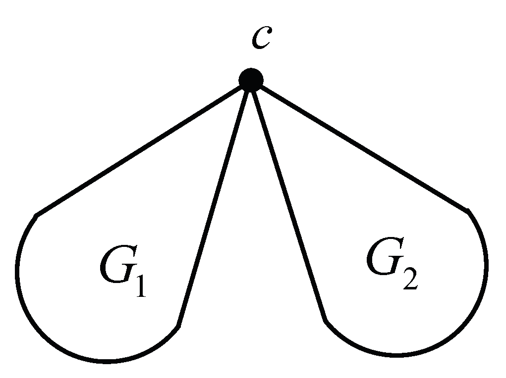
- (a)
- , where are the trees obtained from and by identifying the vertex c;
- (b)
- , where are the trees obtained from and by identifying their vertex c.
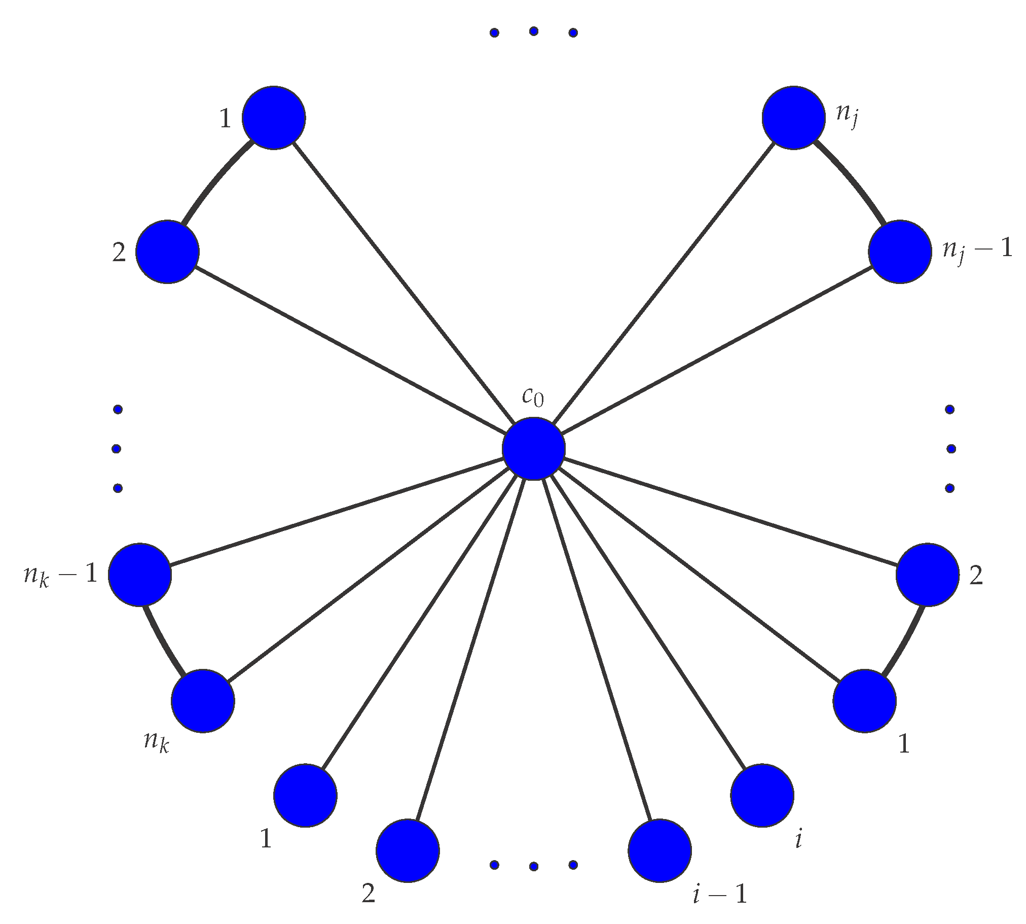
2.4. Further Definitions
3. BC-Subtree Generating Functions of Multi-Fan Graphs
- (i)
- ones not containing the center ;
- (ii)
- ones containing the center .
- (resp. ) is the set of subtrees (resp. BC-subtrees) that contain , but not or ;
- (resp. ) is the set of subtrees (resp. BC-subtrees) that contain , , but not ;
- (resp. ) is the set of subtrees (resp. BC-subtrees) that contain , , but not ;
- (resp. ) is the set of subtrees (resp. BC-subtrees) that contain , and .
- (a)
- ;
- (b)
- , where is the tree obtained from , by attaching an edge at vertex ;
- (c)
- The set can be written as
- (d)
- Evidently, each must not contain the edge . We further consider these subtrees by cases of containing edges but not , for , which can be rewritten as:
4. BC-Subtree Generating Functions of Multi-Wheel Graphs
- (i)
- ones not containing the center ;
- (ii)
- ones containing the center .
- (resp. ) is the set of subtrees (resp. BC-subtrees) that contain , but not ;
- (resp. ) is the set of subtrees (resp. BC-subtrees) that contains and , but neither nor ;
- (resp. ) is the set of subtrees (resp. BC-subtrees) that contain , and , but not ;
- (resp. ) is the set of subtrees (resp. BC-subtrees) that contain , , and ;
- (resp. ) is the set of subtrees (resp. BC-subtrees) that contain , and , but not .
- (resp. ) is the set of subtrees (resp. BC-subtrees) that contain , but not or ;
- (resp. ) is the set of subtrees (resp. BC-subtrees) that contain and , but not ;
- (resp. ) is the set of subtrees (resp. BC-subtrees) that contain , and ;
- (resp. ) is the set of subtrees (resp. BC-subtrees) that contain and , but not .
5. The Behavior of the BC-Subtrees
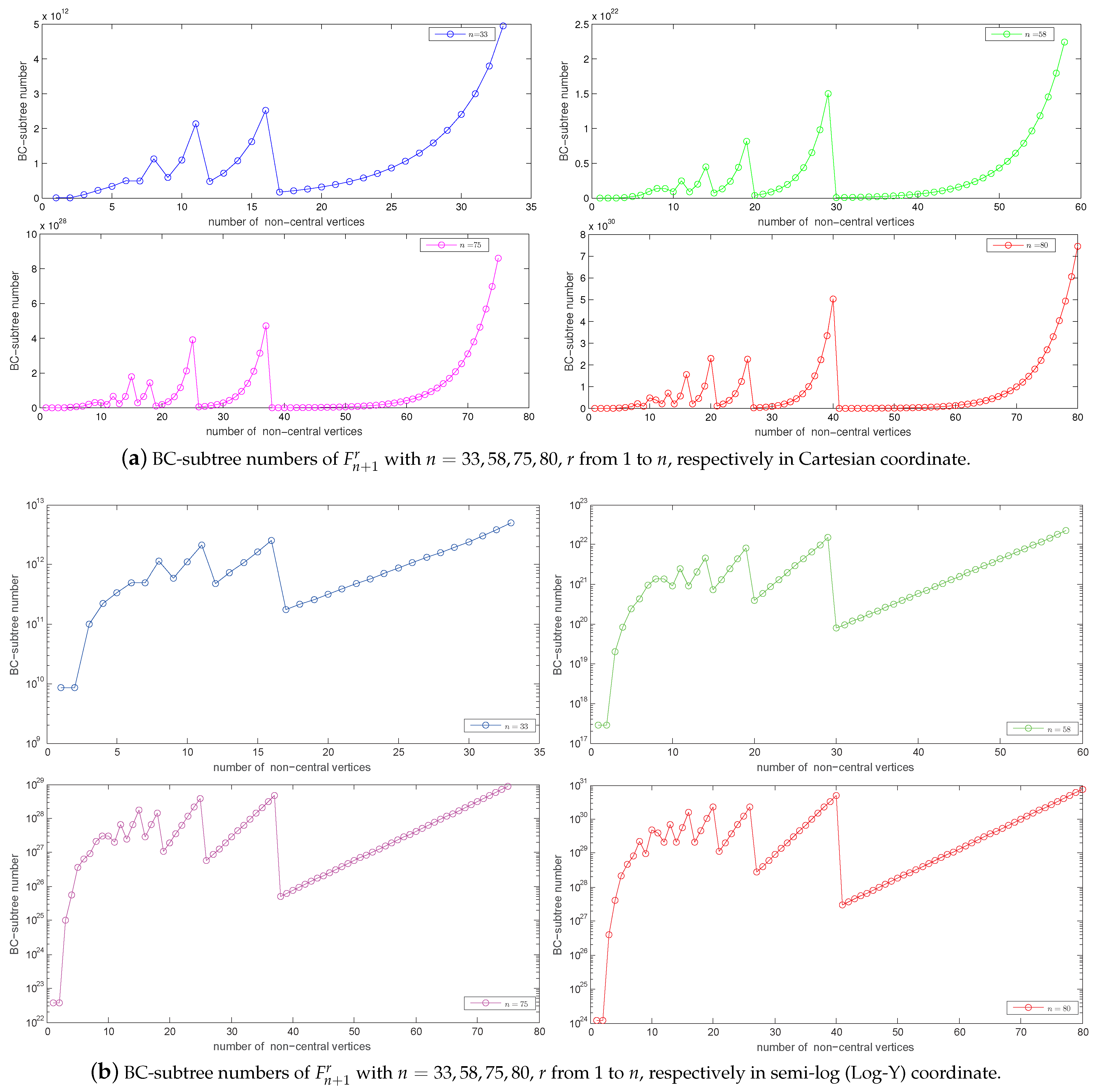
5.1. BC-Subtree Number of
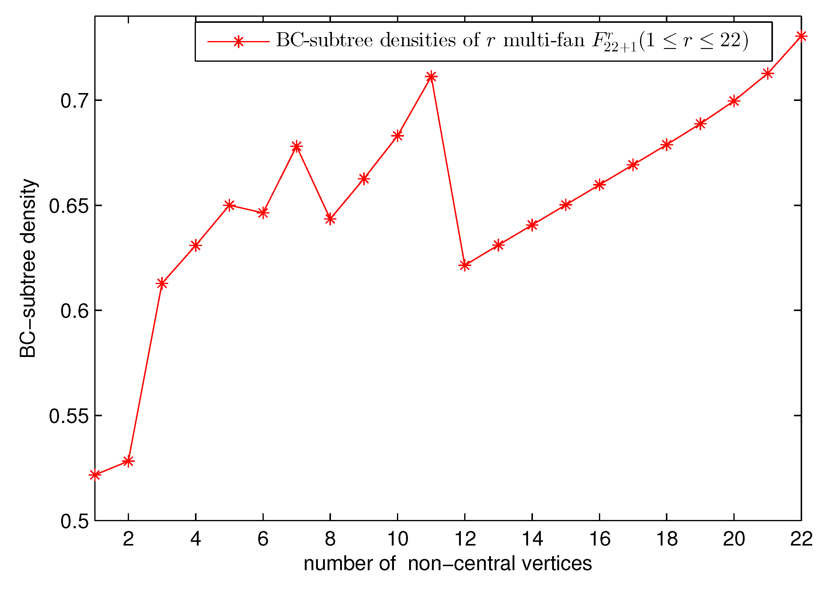
5.2. BC-Subtree Density
6. Concluding Remarks
Author Contributions
Funding
Conflicts of Interest
References
- Wiener, H. Structural determination of paraffin boiling points. J. Am. Chem. Soc. 1947, 1, 17–20. [Google Scholar] [CrossRef]
- Xu, K.; Das, K.C. On Harary index of graphs. Discret. Appl. Math. 2011, 159, 1631–1640. [Google Scholar] [CrossRef]
- Sun, Q.; Ikica, B.; Škrekovski, R.; Vukašinović, V. Graphs with a given diameter that maximise the Wiener index. Appl. Math. Comput. 2019, 356, 438–448. [Google Scholar] [CrossRef]
- Binu, M.; Mathew, S.; Mordeson, J. Wiener index of a fuzzy graph and application to illegal immigration networks. Fuzzy Sets Syst. 2020, 384, 132–147. [Google Scholar] [CrossRef]
- Dimitrov, D.; Milosavljević, N. Efficient computation of trees with minimal atom-bond connectivity Index revisited. Match Commun. Math. Comput. Chem. 2018, 79, 431–450. [Google Scholar]
- Milovanović, E.; Milovanović, I.; Matejić, M. Remark on spectral study of the geometric–arithmetic index and some generalizations. Appl. Math. Comput. 2018, 334, 206–213. [Google Scholar] [CrossRef]
- Sah, A.; Sawhney, M. On the Discrepancy Between Two Zagreb Indices. Discret. Math. 2018, 341, 2575–2589. [Google Scholar] [CrossRef]
- Zhang, X.; Yang, Y.; Wang, H.; Zhang, X. Maximum atom-bond connectivity index with given graph parameters. Discret. Appl. Math. 2016, 215, 208–217. [Google Scholar] [CrossRef]
- Chen, X.; Zhang, J.; Sun, W. On the Hosoya index of a family of deterministic recursive trees. Phys. Stat. Mech. Its Appl. 2017, 465, 449–453. [Google Scholar] [CrossRef]
- De Ita Luna, G.; Raymundo Marcial-Romero, J.; Bello Lopez, P.; Contreras Gonzalez, M. Linear-time algorithms for computing the Merrifield-Simmons index on polygonal trees. Match Commun. Math. Comput. Chem. 2018, 79, 55–78. [Google Scholar]
- Huang, Y.; Shi, L.; Xu, X. The Hosoya index and the Merrifield–Simmons index. J. Math. Chem. 2018, 56, 3136–3146. [Google Scholar] [CrossRef]
- Yan, W.; Yeh, Y. Enumeration of subtrees of trees. Theor. Comput. Sci. 2006, 369, 256–268. [Google Scholar] [CrossRef]
- Yang, Y.; Liu, H.; Wang, H.; Makeig, S. Enumeration of BC-subtrees of trees. Theor. Comput. Sci. 2015, 580, 59–74. [Google Scholar] [CrossRef]
- Lin, W.; Chen, J.; Wu, Z.; Dimitrov, D.; Huang, L. Computer search for large trees with minimal ABC index. Appl. Math. Comput. 2018, 338, 221–230. [Google Scholar] [CrossRef]
- Wagner, S.G. Correlation of graph-theoretical indices. SIAM J. Discret. Math. 2007, 21, 33–46. [Google Scholar] [CrossRef]
- Yang, Y.; Liu, H.; Wang, H.; Deng, A.; Magnant, C. On Algorithms for Enumerating Subtrees of Hexagonal and Phenylene Chains. Comput. J. 2017, 60, 690–710. [Google Scholar] [CrossRef]
- Zhou, Q.; Wang, L.; Lu, Y. Wiener index and Harary index on Hamilton-connected graphs with large minimum degree. Discret. Appl. Math. 2018, 247, 180–185. [Google Scholar] [CrossRef]
- Joiţa, D.M.; Jäntschi, L. Extending the characteristic polynomial for characterization of C20 fullerene congeners. Mathematics 2017, 5, 84. [Google Scholar] [CrossRef]
- García-Pereira, I.; Zanni, R.; Galvez-Llompart, M.; Galvez, J.; García-Domenech, R. DesMol2, an effective tool for the construction of molecular libraries and its application to QSAR using molecular topology. Molecules 2019, 24, 736. [Google Scholar] [CrossRef]
- Bonchev, D. The overall Wiener index–a new tool for characterization of molecular topology. J. Chem. Inf. Model. 2001, 41, 582–592. [Google Scholar]
- Bonchev, D. Chapter 3—On the Concept for Overall Topological Representation of Molecular Structure. In Advances in Mathematical Chemistry and Applications; Basak, S.C., Restrepo, G., Villaveces, J.L., Eds.; Bentham Science Publishers: Sharjah, UAE, 2015; pp. 42–75. [Google Scholar]
- Yang, Y.; Sun, X.J.; Cao, J.Y.; Wang, H.; Zhang, X.D. The expected subtree number index in random polyphenylene and spiro chains. Discret. Appl. Math. 2020, 285, 483–492. [Google Scholar] [CrossRef]
- Sills, A.V.; Wang, H. The minimal number of subtrees of a tree. Graphs Comb. 2015, 31, 255–264. [Google Scholar] [CrossRef]
- Székely, L.; Wang, H. On subtrees of trees. Adv. Appl. Math. 2005, 34, 138–155. [Google Scholar] [CrossRef]
- Zhang, X.; Zhang, X. The minimal number of subtrees with a given degree sequence. Graphs Comb. 2015, 31, 309–318. [Google Scholar] [CrossRef]
- Zhang, X.; Zhang, X.; Gray, D.; Wang, H. The number of subtrees of trees with given degree sequence. J. Graph Theory 2013, 73, 280–295. [Google Scholar] [CrossRef]
- Harary, F.; Plummer, M. On the core of a graph. Proc. Lond. Math. Soc. 1967, 17, 249–257. [Google Scholar] [CrossRef]
- Harary, F.; Prins, G. The block-cutpoint-tree of a graph. Publ. Math. Debr. 1966, 13, 103–107. [Google Scholar]
- Nakayama, T.; Fujiwara, Y. BCT Representation of Chemical Structures. J. Chem. Inf. Comput. Sci. 1980, 20, 23–28. [Google Scholar] [CrossRef]
- Nakayama, T.; Fujiwara, Y. Computer representation of generic chemical structures by an extended block-cutpoint tree. J. Chem. Inf. Comput. Sci. 1983, 23, 80–87. [Google Scholar] [CrossRef]
- Frederickson, G.N.; Hambrusch, S.E. Planar linear arrangements of outerplanar graphs. IEEE Trans. Circuits Syst. 1988, 35, 323–333. [Google Scholar] [CrossRef]
- Wada, K.; Luo, Y.; Kawaguchi, K. Optimal fault-tolerant routings for connected graphs. Inf. Process. Lett. 1992, 41, 169–174. [Google Scholar] [CrossRef]
- Gagarin, A.; Labelle, G. Two-connected graphs with prescribed three-connected components. Adv. Appl. Math. 2009, 43, 46–74. [Google Scholar] [CrossRef][Green Version]
- Heath, L.; Pemmaraju, S. Stack and queue layouts of directed acyclic graphs: Part II. SIAM J. Comput. 1999, 28, 1588–1626. [Google Scholar] [CrossRef][Green Version]
- Paton, K. An algorithm for the blocks and cutnodes of a graph. Commun. ACM 1971, 14, 468–475. [Google Scholar] [CrossRef]
- Misiolek, E.; Chen, D.Z. Two flow network simplification algorithms. Inf. Process. Lett. 2006, 97, 197–202. [Google Scholar] [CrossRef]
- Fox, D. Block cutpoint decomposition for markovian queueing systems. Appl. Stoch. Model. Data Anal. 1988, 4, 101–114. [Google Scholar] [CrossRef]
- Barefoot, C. Block-cutvertex trees and block-cutvertex partitions. Discret. Math. 2002, 256, 35–54. [Google Scholar] [CrossRef][Green Version]
- Mkrtchyan, V. On trees with a maximum proper partial 0–1 coloring containing a maximum matching. Discret. Math. 2006, 306, 456–459. [Google Scholar] [CrossRef]
- Yang, Y.; Liu, H.; Wang, H.; Sun, S. On Spiro and polyphenyl hexagonal chains with respect to the number of BC-subtrees. Int. J. Comput. Math. 2017, 94, 774–799. [Google Scholar] [CrossRef]
- Yang, Y.; Liu, H.; Wang, H.; Feng, S. On algorithms for enumerating BC-subtrees of unicyclic and edge-disjoint bicyclic graphs. Discret. Appl. Math. 2016, 203, 184–203. [Google Scholar] [CrossRef]
- Yang, Z.; Liu, Y.; Li, X.Y. Beyond trilateration: On the localizability of wireless ad hoc networks. IEEE/ACM Trans. Netw. (ToN) 2010, 18, 1806–1814. [Google Scholar] [CrossRef]
- Tu, J.; Zhou, Y.; Su, G. A kind of conditional connectivity of Cayley graphs generated by wheel graphs. Appl. Math. Comput. 2017, 301, 177–186. [Google Scholar] [CrossRef]
- Liu, X.; Zhang, Y.; Gui, X. The multi-fan graphs are determined by their Laplacian spectra. Discret. Math. 2008, 308, 4267–4271. [Google Scholar] [CrossRef]
- Zhang, Y.; Liu, X.; Yong, X. Which wheel graphs are determined by their Laplacian spectra? Comput. Math. Appl. 2009, 58, 1887–1890. [Google Scholar] [CrossRef]
- Kumar, A.; Sarkar, R. Hilbert series of binomial edge ideals. Commun. Algebra 2019, 47, 3830–3841. [Google Scholar] [CrossRef]
- Yang, Y.; Wang, A.; Wang, H.; Zhao, W.T.; Sun, D.Q. On Subtrees of Fan Graphs, Wheel Graphs, and “Partitions” of Wheel Graphs Under Dynamic Evolution. Mathematics 2019, 5, 472. [Google Scholar] [CrossRef]
- Cao, S.; Dehmer, M.; Shi, Y. Extremality of degree-based graph entropies. Inf. Sci. 2014, 278, 22–33. [Google Scholar] [CrossRef]
- Székely, L.A.; Wang, H. Extremal values of ratios: Distance problems vs. subtree problems in trees. Electron. J. Comb. 2013, 20, P67. [Google Scholar] [CrossRef]
- Wang, H. The extremal values of the Wiener index of a tree with given degree sequence. Discret. Appl. Math. 2008, 156, 2647–2654. [Google Scholar] [CrossRef]
- Allen, B.; Lippner, G.; Chen, Y.T.; Fotouhi, B.; Momeni, N.; Yau, S.T.; Nowak, M.A. Evolutionary dynamics on any population structure. Nature 2017, 544, 227. [Google Scholar] [CrossRef]


| 3 | 16 | 19 | 32,983,507 | 35 | 44,956,112,462,965 |
| 4 | 51 | 20 | 79,507,829 | 36 | 109,018,361,948,171 |
| 5 | 131 | 21 | 191,713,586 | 37 | 264,446,533,681,852 |
| 6 | 340 | 22 | 462,509,681 | 38 | 641,651,556,370,739 |
| 7 | 841 | 23 | 1,116,289,936 | 39 | 1,557,326,469,215,175 |
| 8 | 2067 | 24 | 2,695,367,516 | 40 | 3,780,724,965,944,533 |
| 9 | 5026 | 25 | 6,510,870,551 | 41 | 9,180,821,777,073,118 |
| 10 | 12,147 | 26 | 15,733,892,896 | 42 | 22,299,504,128,100,416 |
| 11 | 29,305 | 27 | 38,036,865,379 | 43 | 54,176,661,898,045,614 |
| 12 | 70,508 | 28 | 91,989,932,352 | 44 | 131,652,455,330,130,629 |
| 13 | 169,664 | 29 | 222,555,514,089 | 45 | 319,993,939,502,205,010 |
| 14 | 407,988 | 30 | 538,634,836,904 | 46 | 777,941,764,394,823,593 |
| 15 | 981,517 | 31 | 1,304,079,385,141 | 47 | 1,891,653,259,171,010,731 |
| 16 | 2,361,611 | 32 | 3,158,367,596,891 | 48 | 4,600,677,046,844,511,460 |
| 17 | 5,684,920 | 33 | 7,651,840,948,554 | 49 | 11,191,401,704,559,183,703 |
| 18 | 13,690,201 | 34 | 18,544,255,820,839 | 50 | 27,228,679,901,334,157,132 |
| 1 | 50,331,603 | 4,194,281 | 0.5217415249997297 |
| 2 | 53,106,905 | 4,371,427 | 0.5282018593848684 |
| 3 | 285,872,367 | 20,279,905 | 0.6128841997941354 |
| 4 | 473,222,721 | 32,609,837 | 0.6309415442046974 |
| 5 | 744,621,994 | 49,805,736 | 0.6500229070874051 |
| 6 | 717,819,208 | 48,287,696 | 0.6463247031419493 |
| 7 | 1,460,830,943 | 93,663,206 | 0.6781146144633033 |
| 8 | 703,383,187 | 47,521,825 | 0.6435333174946917 |
| 9 | 1,091,991,586 | 71,647,232 | 0.662661958015046 |
| 10 | 1,742,448,206 | 110,913,152 | 0.6830444927953532 |
| 11 | 3,063,687,819 | 187,270,907 | 0.7112894381260796 |
| 12 | 448,577,818 | 31,383,926 | 0.6214449840120178 |
| 13 | 556,641,580 | 38,350,250 | 0.6310730132420768 |
| 14 | 690,781,206 | 46,878,694 | 0.6406741083329001 |
| 15 | 857,549,247 | 57,340,131 | 0.6502383098769903 |
| 16 | 1,065,571,361 | 70,221,005 | 0.6597625540775962 |
| 17 | 1,326,780,941 | 86,192,884 | 0.6692678698344194 |
| 18 | 1,659,024,388 | 106,256,288 | 0.678844485235874 |
| 19 | 2,091,899,843 | 132,053,383 | 0.6887530256377947 |
| 20 | 2,680,301,328 | 166,568,142 | 0.6996226226010619 |
| 21 | 3,536,505,225 | 215,724,226 | 0.7127669413407951 |
| 22 | 4,906,885,913 | 292,065,325 | 0.73046283663632 |
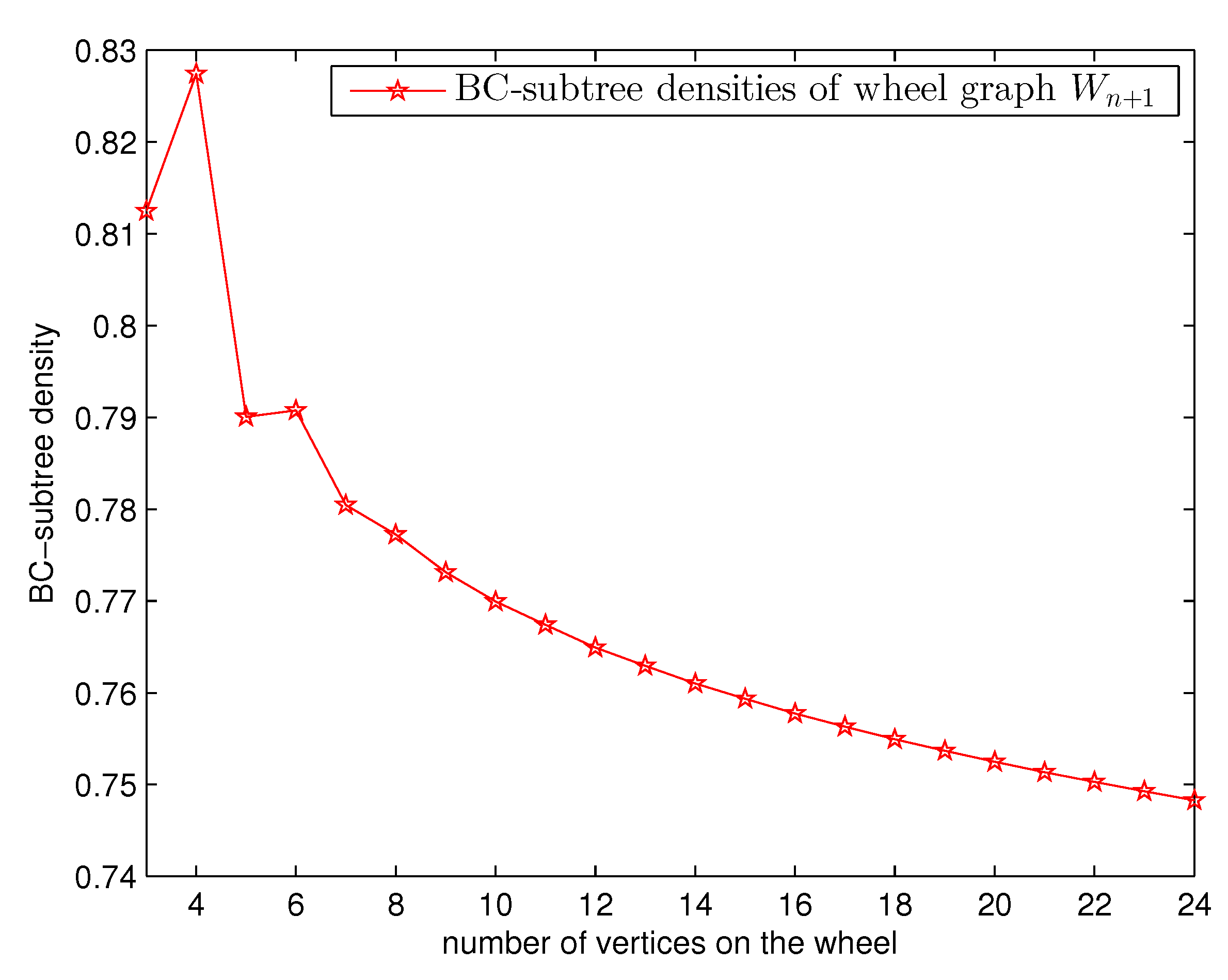
| 3 | 52 | 0.8125 | 14 | 4,657,240 | 0.7610093107313614 |
| 4 | 211 | 0.8274509803921568 | 15 | 11,924,887 | 0.7593403247218337 |
| 5 | 621 | 0.7900763358778626 | 16 | 30,421,819 | 0.7577533999908885 |
| 6 | 1882 | 0.7907563025210084 | 17 | 77,392,093 | 0.7563098024637501 |
| 7 | 5251 | 0.7804696789536266 | 18 | 196,372,903 | 0.7549499052182229 |
| 8 | 14,459 | 0.7772402300704188 | 19 | 497,180,696 | 0.7536807653594871 |
| 9 | 38,857 | 0.7731197771587743 | 20 | 1,256,299,889 | 0.7524833703900728 |
| 10 | 102,877 | 0.7699394538120149 | 21 | 3,168,978,905 | 0.7513525707135758 |
| 11 | 269,864 | 0.7674003298640732 | 22 | 7,981,278,895 | 0.7502807835703772 |
| 12 | 701,132 | 0.7649235656837631 | 23 | 20,073,455,736 | 0.749262321576641 |
| 13 | 1,812,214 | 0.7629423869698766 | 24 | 50,423,103,620 | 0.7482928145521214 |
Publisher’s Note: MDPI stays neutral with regard to jurisdictional claims in published maps and institutional affiliations. |
© 2020 by the authors. Licensee MDPI, Basel, Switzerland. This article is an open access article distributed under the terms and conditions of the Creative Commons Attribution (CC BY) license (http://creativecommons.org/licenses/by/4.0/).
Share and Cite
Yang, Y.; Li, L.; Wang, W.; Wang, H. On BC-Subtrees in Multi-Fan and Multi-Wheel Graphs. Mathematics 2021, 9, 36. https://doi.org/10.3390/math9010036
Yang Y, Li L, Wang W, Wang H. On BC-Subtrees in Multi-Fan and Multi-Wheel Graphs. Mathematics. 2021; 9(1):36. https://doi.org/10.3390/math9010036
Chicago/Turabian StyleYang, Yu, Long Li, Wenhu Wang, and Hua Wang. 2021. "On BC-Subtrees in Multi-Fan and Multi-Wheel Graphs" Mathematics 9, no. 1: 36. https://doi.org/10.3390/math9010036
APA StyleYang, Y., Li, L., Wang, W., & Wang, H. (2021). On BC-Subtrees in Multi-Fan and Multi-Wheel Graphs. Mathematics, 9(1), 36. https://doi.org/10.3390/math9010036