Extended VIKOR-QUALIFLEX Method Based on Trapezoidal Fuzzy Two-Dimensional Linguistic Information for Multiple Attribute Decision-Making with Unknown Attribute Weight

Abstract

Considering the advantages of trapezoid fuzzy two-dimensional linguistic variables (TrF2DLVs), which can not only accurately describe the qualitative evaluation but also use qualitative linguistic variables (LVs) to describe the confidence level of this evaluation in the second dimension, this paper proposes a novel method based on trapezoidal fuzzy two-dimensional linguistic information to solve multiple attribute decision-making (MADM) problems with unknown attribute weight. First, a combination weight model is constructed, which covers a subjective weight determination model based on the proposed trapezoidal fuzzy two-dimensional linguistic best-worst method (TrF2DL-BWM) and an objective weight determination model based on the proposed CRITIC method. Then, in order to accurately rank the alternatives, an extended VIKOR-QUALIFLEX method is proposed, which can measure the concordance index of each ranking combination by means of group utility and individual maximum regret value of each evaluation alternative. Finally, a practical problem of lean management assessment for industrial residential projects is solved by the proposed method, and the effectiveness and advantages of the method are demonstrated by comparative analysis and discussion.

1. Introduction

With the continuous development of society, management decision-making has become increasingly important. How to make a wise decision on some major issues is related to the long-term development of the government, enterprises, and individuals. In this way, the multiple attribute decision-making (MADM) method, that is to evaluate and make decisions on multiple alternatives through multiple attributes of objectives, plays a key role. Scholars have also been studying and discussing this topic for a long time [1,2,3,4,5].

For MADM, the representation model of decision information is a primary and crucial research topic. Generally, decision attributes are divided into two forms: quantitative attributes and qualitative attributes. In quantitative evaluation, crisp number is the initial evaluation tool to express the exact information. However, in the complex decision-making process, some evaluation information may be uncertain. Therefore, Zadeh [6] put forward a novel concept, fuzzy set (FS), which is used to describe the quantitative evaluation of an objective in the form of membership degree. With the rise of fuzzy sets, all kinds of extended fuzzy information begin to appear, such as interval fuzzy number, triangular fuzzy number, and trapezoidal fuzzy number (TrFN). Among them, TrFN is the most generalized and accurate form, which can be reduced to other fuzzy information forms by adjusting membership function, so it has been paid great attention [7,8]. In addition, in terms of qualitative evaluation, the linguistic variables (LVs) introduced by Zadeh [9] promote the convenient expression of qualitative information, which is more in line with human evaluation habits. Then, some scholars point out that a single linguistic term (LT) is not enough to accurately model the qualitative evaluation information, so some extended linguistic information forms begin to emerge, such as two-dimensional linguistic variables (2DLVs) [10], hesitant fuzzy linguistic term sets [11], probabilistic linguistic term sets [12,13], and so on. However, it is worth noting that in the real complex decision-making environment, if people want to describe some uncertain information more accurately and completely, it is necessary to consider both qualitative and quantitative expressions. Inspired by 2DLVs, Li et al. [14] put forward the trapezoid fuzzy two-dimensional linguistic variables (TrF2DLVs), which can describe the evaluation information through two dimensions. In the first dimension, the TrFN is used to present the qualitative evaluation of the object, and in the second dimension, the LV is used to describe the degree of certainty of the evaluation produced by the first dimension. In this way, the TrF2DLVs can model the uncertain evaluation information more accurately through the combination of quantitative and qualitative tools. Based on the unique advantages of TrF2DLVs, they have been gradually concerned and studied in recent years [14,15,16].

The determination of attribute weight is the second problem and challenge of MADM. In most of the MADM problems, the weight of attributes is given directly, which is not only unscientific but also relatively reckless, because of which the evaluation results cannot reflect the real evaluation situation. Therefore, many scholars began to study the weight model, which can be divided into two categories, one is the determination of subjective attribute weight, whereas the other is the determination of objective attribute weight. The research of subjective weight model mainly focuses on AHP method [17], SWARA method [18], and BWM [4]. In particular, it is necessary to point out that the SWARA method is used because of its simplicity and a small number of steps. However, it does not have the ability to determine the consistency degree of the comparisons. The traditional AHP method determines the priority relationship of attributes by pairwise comparison. However, once the number of attributes is large, the number of pairwise comparison will be more, which will easily lead to the inconsistency of preference matrix. In order to simplify the complexity of AHP and improve the logical rationality of evaluation matrix, Rezaei [4] contributed the best-worst method (BWM), which only needs to determine the best and worst attributes, and then compare with other attributes. In view of the advantages of BWM, it has been widely used in MADM. For example, Guo and Zhao [2] proposed that the fuzzy BWM is to solve the issues under fuzzy environment, and defined the consistency ratio for fuzzy BWM; Brunelli and Rezaei [1] introduced a new metric into the framework of BWM to deal with MADM problems; Kumar et al. [19] presented a hybrid BWM and VIKOR method to evaluate green performance of the airports; and Muravev and Mijic [20] put forward a novel BWM-MABAC Model for integrated provider selection problems. For the determination of objective weight method, there are various weight models, such as entropy weight model [21], deviation maximization model [22], grey correlation analysis model [23], bidirectional projection model [24], and CRITIC model [25]. Among them, the CRITIC method has a very unique advantage, which can quantify contrast intensity and conflict to measure the weight of attributes, and further make the evaluation results easier to distinguish the priority relationship. Thus, CRITIC method has been paid more and more attention in MADM. For example, some TOPSIS-CRITIC models are presented to solve practical application problems in [25,26]; Žižović et al. [27] proposed a modified CRITIC method to determine criteria weight coefficients, and so forth.

For the research of MADM method, the core research point is about the ranking method. Generally speaking, ranking methods are divided into two types: one is based on information aggregation operators, and the other is traditional ranking method based on various information measures. With the increasing functions and features of information aggregation operators, the first kind of ranking methods have received special attention because they are easy to operate. For instance, Liu et al. [28] studied the MADM method based on the interval type-2 fuzzy partitioned Bonferroni mean operator for green supplier selection problem, which can consider the complex correlation between two attributes in different class groups; Liu and Li introduced the trapezoidal fuzzy two-dimensional linguistic power generalized Hamy mean operator considering the correlation among multiple attributes to deal with MADM problem. However, it is undeniable that although the MADM methods based on aggregation operator are simple, it may cause information loss in the decision-making process. Therefore, this study advocates to use the traditional ranking method. For example, the TOPSIS [23], MABAC [29], and VIKOR [19,30] methods can consider the distance from the alternatives to the positive and negative ideal solutions; the MAIRCA method [31] can reflect in determining the gap between the ideal and the empirical ponders; the MARCOS method [32] can determine the utility functions on the basis of the defined relationships between alternatives and reference values (ideal and anti-ideal alternatives), and the COPRAS method [33] can determine the relative significance values of alternatives based on the relationships between maximizing and minimizing indexes. Among these methods, the VIKOR method has an obvious advantage, i.e., it can use the group utility value and individual maximum regret value to find a compromise solution. In addition, the ELECTRE [7], PROMETHEE [34], and QUALIFLEX [35] method can measure the priority of alternatives by considering the possibility degree, preference index, and concordance index between alternatives, respectively, and then get the ranking results. Although these traditional methods have many steps, the evaluation results obtained by them are more accurate and more stable than those obtained by those methods based on aggregation operators.

Although TrF2DLVs have unique advantages in information expression, its research and application in MADM has not attracted enough attention from experts and scholars. Some of the existing research results have some positive highlights, but there are still some shortcomings that need to be improved. For example, the existing MADM methods based on trapezoidal fuzzy two-dimensional linguistic information do not consider the determination model of subjective weight. Although the power aggregation operator used by Li et al. in [14] and Liu and Li [15] can calculate the objective weight of attribute value, its main purpose is to deal with the problem that the evaluation information contains extreme evaluation values. The corresponding problem is that all evaluation values tend to be the same, which weakens the differentiation of priority among different alternatives. In addition, it is not scientific to merely rely on the subjective weight or objective weight of attributes to rank the alternatives. This is because the subjective weight combines the experience, preference and knowledge background of decision-makers (DMs), while the objective weight represents some objective information of the evaluation data itself. Moreover, for the research of ranking methods, the existing MADM methods based on the TrF2DLVs are constructed based on various aggregation operators, and they are extremely unstable in response to the attribute weights, which is not desirable for some evaluation problems. Through the literature review, we can find that BWM can effectively calculate the subjective weights of attributes in MADM problems, while CRITIC method has outstanding advantages in obtaining objective weights of attributes. However, the application results of these methods in fuzzy environment are relatively few. In addition, the VIKOR method is a very effective sorting tool, but it still needs some improvement because it cannot get the unique solution. In view of these motivations, the innovation and contributions of this study mainly focuses on the following aspects:

(1)

Some basic concepts about TrF2DLVs are introduced, including expectation value based on scale function, distance measure, and trapezoidal fuzzy two-dimensional linguistic preference relation (TrF2DLPR).

(2)

A combination weight model based on trapezoidal fuzzy two-dimensional linguistic information is proposed to solve the MADM problems with unknown attribute weights, which includes proposing a trapezoidal fuzzy two-dimensional linguistic best-worst method (TrF2DL-BWM) to determine the subjective attribute weight, proposing a CRITIC method to determine the objective attribute weight, and proposing a method based on the maximum comprehensive evaluation value to determine the combination weight.

(3)

An extended VIKOR-QUALIFLEX method based on TrF2DLVs is presented to solve MADM problems, which can measure the concordance index of each ranking combination by means of group utility and individual maximum regret value of each evaluation alternative, and get more stable evaluation result.

(4)

A practical application of lean management assessment for industrial residential projects is solved by the proposed method.

The following sections of this study can be presented as below. Section 2 introduces some basic concepts needed in this study. Section 3 proposes the model of the weights of attributes for MADM based on trapezoidal fuzzy two-dimensional linguistic information. Section 4 presents an extended VIKOR-QUALIFLEX method for TrF2DLVs to deal with MADM problems. Section 5 solves the practical problems of lean management evaluation of the industrial residential projects, verifies the effectiveness of the proposed method, and demonstrates its advantages. In Section 6, the conclusions are given.

2. Preliminaries

This section will introduce some basic concepts needed in this study, including TrFNs, linguistic term sets (LTSs), TrF2DLV, and TrF2DLPRs.

2.1. Trapezoidal Fuzzy Numbers

Definition 1. 

[36] Let $\tilde{t}=\left(t^L,t^{ML},t^{MU},t^U\right)$ which meets the condition $t^L\le t^{ML}\le t^{MU}\le t^U$, and its membership degree function $t\left(x\right)$:$R\in \left[0,1\right]$is defined as below:

$$t\left(x\right)=\{\begin{array}{l}\frac{x-t^L}{t^{ML}-t^L},\hspace{0.17em}\hspace{0.17em}\hspace{0.17em}\hspace{0.17em}\hspace{0.17em}x\in \left(t^L,t^{ML}\right)\\ 1,\hspace{0.17em}\hspace{0.17em}\hspace{0.17em}\hspace{0.17em}\hspace{0.17em}\hspace{0.17em}\hspace{0.17em}\hspace{0.17em}\hspace{0.17em}\hspace{0.17em}\hspace{0.17em}\hspace{0.17em}x\in \left(t^{ML},t^{MU}\right)\\ \hspace{0.17em}\frac{x-t^L}{t^{ML}-t^L},\hspace{0.17em}\hspace{0.17em}\hspace{0.17em}\hspace{0.17em}x\in \left(t^{MU},t^U\right)\\ 0,\hspace{0.17em}\hspace{0.17em}\hspace{0.17em}\hspace{0.17em}\hspace{0.17em}\hspace{0.17em}\hspace{0.17em}\hspace{0.17em}\hspace{0.17em}\hspace{0.17em}\hspace{0.17em}\hspace{0.17em}x\in \left(-\infty ,t^L\right)\cup \left(t^U,+\infty \right),\hspace{0.17em}\end{array}$$

(1)

then $\tilde{t}=\left(t^L,t^{ML},t^{MU},t^U\right)$can be called as a trapezoidal fuzzy number (TrFN), where the element $x\in R$ of $\tilde{t}$is real number, and its membership function $t\left(x\right)$, a regular and continuous convex function, stands for the degree of element x to the FS $\tilde{t}$. Obviously, when $t^L<t^{ML}=t^{MU}<t^U$, then the TrFN $\tilde{t}$ reduces to a triangular fuzzy number; when $t^L=t^{ML}=t^{MU}=t^U$, then the TrFN $\tilde{t}$ reduces to a crisp number.

Suppose ${\tilde{t}}_1=\left(t_1^L,t_1^{ML},t_1^{MU},t_1^U\right)$ and ${\tilde{t}}_2=\left(t_2^L,t_2^{ML},t_2^{MU},t_2^U\right)$ are any two TrFNs, then their operational rules are presented as below [14,36]:

$${\tilde{t}}_1+{\tilde{t}}_2=\left(t_1^L+t_2^L,t_1^{ML}+t_2^{ML},t_1^{MU}+t_2^{MU},t_1^U+t_2^U\right)$$

(2)

$${\tilde{t}}_1-{\tilde{t}}_2=\left(t_1^L-t_2^L,t_1^{ML}-t_2^{ML},t_1^{MU}-t_2^{MU},t_1^U-t_2^U\right)$$

(3)

$${\tilde{t}}_1{\tilde{t}}_2=\left(t_1^L{t}_2^L,t_1^{ML}{t}_2^{ML},t_1^{MU}{t}_2^{MU},t_1^U{t}_2^U\right)$$

(4)

$${\tilde{t}}_1/{\tilde{t}}_2=\left(t_1^L/t_2^L,t_1^{ML}/t_2^{ML},t_1^{MU}/t_2^{MU},t_1^U/t_2^U\right)$$

(5)

$$\gamma {\tilde{t}}_1=\left(\gamma t_1^L,\gamma t_1^{ML},\gamma t_1^{MU},\gamma t_1^U\right),\gamma \ge 0$$

(6)

$${\left({\tilde{t}}_1\right)}^{\gamma }=\left({\left(t^L\right)}^{\gamma },{\left(t^{ML}\right)}^{\gamma },{\left(t^{MU}\right)}^{\gamma },{\left(t^U\right)}^{\gamma }\right),\hspace{0.17em}\gamma \ge 0.$$

(7)

The distance measure between ${\tilde{t}}_1$ and ${\tilde{t}}_2$ is presented as below:

$$d\left({\tilde{t}}_1,{\tilde{t}}_2\right)=\sqrt{\left[{\left(t_1^L-t_2^L\right)}^2+{\left(t_1^{ML}-t_2^{ML}\right)}^2+{\left(t_1^{MU}-t_2^{MU}\right)}^2+{\left(t_1^U-t_2^U\right)}^2\right]/4}$$

(8)

2.2. Linguistic Term Sets

Let $S=\left\{s_{\epsilon }|\epsilon =0,1,\dots ,2\tau \right\}$ be a finite and totally ordered discrete LTS with odd cardinality, where $s_{\epsilon }$ represents a possible value for a LV; the term must satisfy these properties [37]:

(i)

The set is ordered: $s_{\epsilon }<s_k$ if and only if $\epsilon <k$;

(ii)

There is a negation operator: Neg ($s_{\epsilon }$) = $s_{2\tau -\epsilon }$;

(iii)

If $\epsilon \le k$, then $\max \left\{s_{\epsilon },s_k\right\}=s_k$;

(iv)

If $\epsilon \le k$, then $\min \left\{s_{\epsilon },s_k\right\}=s_{\epsilon }$.

Definition 2. 

[38]: For an LTS $S=\left\{s_{\epsilon }|\epsilon =0,1,\dots ,2\tau \right\}$, the linguistic scale function $y\left(\epsilon \right)$ is expressed as:

$$y\left(\epsilon \right)=\frac{\epsilon }{2\tau },\left(\epsilon =0,1,\dots ,2\tau \right),$$

(9)

where $y\left(\epsilon \right)\in \left[0,1\right]$ and the linguistic scale function can construct a mapping relationship between the linguistic variable and a crisp number.

Note: the linguistic scale function has been widely studied at this stage 5. To simplify the operation, this study selects the simplest linguistic scale function for application. In addition, different DMs can also choose the appropriate linguistic scale function for some actual problems.

2.3. Trapezoidal Fuzzy Two-Dimensional Linguistic Variables

TrFNs can accurately describe the evaluation information of an objective thing, but sometimes people’s confidence in this evaluation information is not absolute. Inspired by two-dimensional linguistic information [10], Li et al. [14] put forward trapezoidal fuzzy two-dimensional linguistic information to describe the evaluated things. In a TrF2DLV, the first dimension can describe the evaluation information by a TrFN, and the second dimension can model the degree of confidence in this evaluation by a LV. Therefore, TrF2DLVs can express fuzzy information accurately and concretely, thus reducing the distortion of information.

Definition 3. 

[14]: Let $\tilde{t}=\left(t^L,t^{ML},t^{MU},t^U\right)$ be a TrFN and $s_{\epsilon }$ be a LT. If $\tilde{t}$ is used to evaluate alternatives by a DM and $s_{\epsilon }$ is used to express the reliability of the evaluation given by the DM, then the $\chi =\left(\left[t^L,t^{ML},t^{MU},t^U\right],s_{\epsilon }\right)$ can be called as a TrF2DLV.

Suppose ${\chi }_1=\left(\left[t_1^L,t_1^{ML},t_1^{MU},t_1^U\right],s_{{\epsilon }_1}\right)$ and ${\chi }_2=\left(\left[t_2^L,t_2^{ML},t_2^{MU},t_2^U\right],s_{{\epsilon }_2}\right)$ are any two TrF2DLVs, where $t_1^L,t_1^{ML},t_1^{MU},t_1^U,t_2^L,t_2^{ML},t_2^{MU},t_2^U\ge 0$ and ${\epsilon }_1,{\epsilon }_2\in \left\{0,1,\dots ,2\tau \right\}$, then their operational rules can be expressed as below:

$${\chi }_1\oplus {\chi }_2=\left(\left[t_1^L+t_2^L,t_1^{ML}+t_2^{ML},t_1^{MU}+t_2^{MU},t_1^U+t_2^U\right],s_{\min ({\epsilon }_1,{\epsilon }_2)}\right)$$

(10)

$${\chi }_1\otimes {\chi }_2=\left(\left[t_1^L{t}_2^L,t_1^{ML}{t}_2^{ML},t_1^{MU}{t}_2^{MU},t_1^U{t}_2^U\right],s_{\min ({\epsilon }_1,{\epsilon }_2)}\right)$$

(11)

$${\chi }_1/{\chi }_2=\left(\left[t_1^L/t_2^L,t_1^{ML}/t_2^{ML},t_1^{MU}/t_2^{MU},t_1^U/t_2^U\right],s_{\min ({\epsilon }_1,{\epsilon }_2)}\right) \mathrm{where} t_2^L,t_2^{ML},t_2^{MU},t_2^U\ne 0$$

(12)

$$\gamma {\chi }_1=\left(\left[\gamma t_1^L,\gamma t_1^{ML},\gamma t_1^{MU},\gamma t_1^U\right],s_{{\epsilon }_1}\right),\hspace{0.17em}\gamma \ge 0$$

(13)

$${\left({\chi }_1\right)}^{\gamma }=\left(\left[{\left(t_1^L\right)}^{\gamma },{\left(t_1^{ML}\right)}^{\gamma },{\left(t_1^{MU}\right)}^{\gamma },{\left(t_1^U\right)}^{\gamma }\right],s_{{\epsilon }_1}\right),\gamma \ge 0.$$

(14)

For any three TrF2DLVs ${\chi }_1$, ${\chi }_2$, and ${\chi }_3$, they have these properties:

(i)

${\chi }_1\oplus {\chi }_2={\chi }_2\oplus {\chi }_1$;

(ii)

${\chi }_1\otimes {\chi }_2={\chi }_2\otimes {\chi }_1$;

(iii)

${\chi }_1\oplus {\chi }_2\oplus {\chi }_3={\chi }_1\oplus \left({\chi }_2\oplus {\chi }_3\right)$;

(iv)

${\chi }_1\otimes {\chi }_2\otimes {\chi }_3={\chi }_1\otimes \left({\chi }_2\otimes {\chi }_3\right)$;

(v)

${\chi }_1\otimes \left({\chi }_2\oplus {\chi }_3\right)=\left({\chi }_1\otimes {\chi }_2\right)\oplus \left({\chi }_1\otimes {\chi }_3\right)$;

(vi)

${\gamma }_1\left({\chi }_1\oplus {\chi }_2\right)={\gamma }_1{\chi }_1\oplus {\gamma }_1{\chi }_2,{\gamma }_1\ge 0$;

(vii)

$\left({\gamma }_1+{\gamma }_2\right){\chi }_1={\gamma }_1{\chi }_1\oplus {\gamma }_2{\chi }_1,\hspace{0.17em}{\gamma }_1,{\gamma }_2\ge 0$.

Definition 4. 

Suppose$\chi =\left(\left[t^L,t^{ML},t^{MU},t^U\right],s_{\epsilon }\right)$is a TrF2DLV, then the expected value of$\chi$can be defined as below:

$$e\left(\chi \right)=\frac{t^L+t^{ML}+t^{MU}+t^U}{4}\times y\left(\epsilon \right),$$

(15)

where$\epsilon$is the subscript of LT$s_{\epsilon }$and$\epsilon \in \left\{0,1,\dots ,2\tau \right\}$, y is the linguistic scale function, and$y\left(\epsilon \right)=\frac{\epsilon }{2\tau }$in this study. Obviously,$e\left(\chi \right)\in [0,1]$.

Suppose ${\chi }_1=\left(\left[t_1^L,t_1^{ML},t_1^{MU},t_1^U\right],s_{{\epsilon }_1}\right)$ and ${\chi }_2=\left(\left[t_2^L,t_2^{ML},t_2^{MU},t_2^U\right],s_{{\epsilon }_2}\right)$ are any two TrF2DLVs. The comparison rules between ${\chi }_1$ and ${\chi }_2$ can be described as below:

(i)

If $E\left({\chi }_1\right)>E\left({\chi }_2\right)$, the ${\chi }_1\succ {\chi }_2$;

(ii)

If $E\left(\chi \right)<E\left({\chi }_2\right)$, the ${\chi }_1\prec {\chi }_2$;

(iii)

If $E\left({\chi }_1\right)=E\left({\chi }_2\right)$, the ${\chi }_1={\chi }_2$.

Definition 5. 

Suppose${\chi }_1=\left(\left[t_1^L,t_1^{ML},t_1^{MU},t_1^U\right],s_{{\epsilon }_1}\right)$and${\chi }_2=\left(\left[t_2^L,t_2^{ML},t_2^{MU},t_2^U\right],s_{{\epsilon }_2}\right)$are any two TrF2DLVs, the distance measure of these TrF2DLVs is defined as below:

$$d\left({\chi }_1,{\chi }_2\right)=\sqrt{{\left(e\left({\chi }_1\right)-e\left({\chi }_2\right)\right)}^2}=\sqrt{{\left(\frac{t_1^L+t_1^{ML}+t_1^{MU}+t_1^U}{4}\times y\left({\epsilon }_1\right)-\frac{t_2^L+t_2^{ML}+t_2^{MU}+t_2^U}{4}\times y\left({\epsilon }_2\right)\right)}^2},$$

(16)

where$e\left({\chi }_1\right)$and$e\left({\chi }_2\right)$are the expected values of${\chi }_1$and${\chi }_2$, respectively.

Clearly, the distance of TrF2DLVs can satisfy these conditions:

(i)

$0\le d\left({\chi }_1,{\chi }_2\right)\le 1$;

(ii)

If ${\chi }_1={\chi }_2$, then $d\left({\chi }_1,{\chi }_2\right)=1$;

(iii)

$d\left({\chi }_1,{\chi }_2\right)=d\left({\chi }_2,{\chi }_1\right)$;

(iv)

$d\left({\chi }_1,{\chi }_2\right)+d\left({\chi }_2,{\chi }_3\right)\ge d\left({\chi }_1,{\chi }_3\right)$.

2.4. Trapezoidal Fuzzy Two-Dimensional Linguistic Preference Relation

Usually, experts can compare the evaluation subjects in pairs through fuzzy numbers to form a fuzzy preference relationship (FPRs) [39].

For FPRs, R_f, on a set of alternatives A = {A₁, A₂, …, A_n} are represented by a FS on the product set A × A and described by a membership function [40]:

$$u_R:\hspace{0.17em}A\times A\to [0,1]$$

(17)

FPRs can be defined as a matrix $R_f={[f_{ij}]}_{n\times n}$ with $f_{ij}=u_R(A_i,A_j),\forall i,j\in \{1,\dots ,n\}$, and expressed as

$$\begin{array}{l}\hspace{1em}\hspace{1em}\hspace{0.17em}\hspace{0.17em}\hspace{0.17em}\hspace{0.17em}\hspace{0.17em}\hspace{0.17em}\hspace{0.17em}\hspace{0.17em}\hspace{0.17em}{A}_1\hspace{0.17em}\hspace{0.17em}\hspace{0.17em}{A}_2\hspace{0.17em}\hspace{0.17em}\dots \hspace{0.17em}\hspace{0.17em}{A}_n\\ R_f=\begin{array}{c}{A}_1\\ A_2\\ ⋮\\ A_n\end{array}\left[\begin{array}{cccc}{f}_{11}& f_{12}& \dots & f_{1n}\\ f_{21}& f_{22}& \dots & f_{2n}\\ ⋮& ⋮& \ddots & ⋮\\ f_{n1}& f_{n2}& \cdots & f_{nn}\end{array}\right]\end{array}$$

(18)

We use $f_{ij}$ to represent the preference degree of an alternative A_i prefer to A_j:

$$f_{ij}=\{\begin{array}{l}0\hspace{1em}\hspace{1em}\hspace{1em}\hspace{1em}\hspace{0.17em}\hspace{0.17em}\hspace{0.17em}{A}_j\hspace{0.17em}\mathrm{is} \mathrm{absolutely}\hspace{0.17em}\mathrm{better} \mathrm{than} A_i;\\ \in (0,0.5)\hspace{1em}\hspace{1em}{A}_j\hspace{0.17em}\hspace{0.17em}\mathrm{is} \mathrm{better} \mathrm{than} A_i\hspace{0.17em};\\ 0.5\hspace{1em}\hspace{1em}\hspace{1em}\hspace{1em}\hspace{0.17em}\mathrm{indifference}\hspace{0.17em}\mathrm{between}\hspace{0.17em}{A}_i\hspace{0.17em}\mathrm{and}\hspace{0.17em}{A}_j;\\ \in (0.5,1)\hspace{1em}\hspace{1em}\hspace{0.17em}{A}_i\hspace{0.17em}\mathrm{is} \mathrm{better} \mathrm{than} A_j;\\ 1\hspace{1em}\hspace{1em}\hspace{1em}\hspace{1em}\hspace{1em}{A}_i\hspace{0.17em}\mathrm{is} \mathrm{absolutely}\hspace{0.17em}\mathrm{better} \mathrm{than}\hspace{0.17em}{A}_j.\end{array}.$$

For the FPRs, some properties need to be satisfied in R_f: (1) $f_{ij}\ge 0$, (2) $f_{ij}+f_{ji}=1,$$\forall i,j\in \{1,\dots ,n\}$, and (3) $f_{ii}=0.5,\forall i\in \{1,\dots ,n\}$.

Fuzzy preference relation can be more convenient to evaluate things, but fuzzy numbers are not enough to describe the evaluation information in reality accurately. Therefore, TrF2DLVs is introduced into fuzzy preference relation hereof and the concept of TrF2DLPR is given.

Definition 6. 

The TrF2DLPR, R_T, on a set of alternatives A are represented by a matrix on the set A × A, whose elements are formulated by

$$R_T:A\times A\to \chi$$

(19)

$$\begin{array}{l}\hspace{1em}\hspace{1em}\hspace{1em}\hspace{0.17em}\hspace{0.17em}\hspace{0.17em}\hspace{0.17em}\hspace{0.17em}\hspace{0.17em}{A}_1\hspace{0.17em}\hspace{0.17em}\hspace{0.17em}{A}_2\hspace{0.17em}\hspace{0.17em}\dots \hspace{0.17em}\hspace{0.17em}\hspace{0.17em}{A}_n\\ R_T=\begin{array}{c}{A}_1\\ A_2\\ ⋮\\ A_n\end{array}\left[\begin{array}{cccc}{\chi }_{11}& {\chi }_{12}& \dots & {\chi }_{1n}\\ {\chi }_{21}& {\chi }_{22}& \dots & {\chi }_{2n}\\ ⋮& ⋮& \ddots & ⋮\\ {\chi }_{n1}& {\chi }_{n2}& \cdots & {\chi }_{nn}\end{array}\right],\end{array}$$

(20)

The matrix $R_T$ is defined as

where TrF2DLVs ${\chi }_{ij}=\left(\left[t_{ij}^L,t_{ij}^{ML},t_{ij}^{MU},t_{ij}^U\right],s_{{\epsilon }_{ij}}\right)$, ${\chi }_{ji}=\left(\left[1-t_{ij}^U,1-t_{ij}^{MU},1-t_{ij}^{ML},1-t_{ij}^L\right],s_{{\epsilon }_{ij}}\right)$, $\forall i,j\in \{1,2,\dots ,n\}$ and $\forall {\epsilon }_{ij}\in \{1,2,\dots ,m\}$.

Example 1. 

Suppose that a DM evaluates three alternatives$A_1$,$A_2$, and$A_3$by pairwise comparison, and he/she uses a TrF2DLPR to express decision-making information. The LV in the second dimension comes from the LTS$S=\{s_0=\mathrm{very} \mathrm{unfamiliar}, s_1=\mathrm{unfamiliar}, s_2=\mathrm{general} \mathrm{familiar}, s_3=\mathrm{familiar}, s_4=\mathrm{very} \mathrm{familiar}\}.$Then, the evaluation matrix$R_T$can be expressed as follows:

$$\begin{array}{l}\hspace{1em}\hspace{1em}\hspace{0.17em}\hspace{0.17em}\hspace{0.17em}\hspace{0.17em}\hspace{0.17em}\hspace{0.17em}\hspace{1em}\hspace{1em}\hspace{1em}\hspace{1em}\hspace{1em}{A}_1\hspace{0.17em}\hspace{1em}\hspace{1em}\hspace{1em}\hspace{1em}\hspace{1em}\hspace{1em}\hspace{1em}\hspace{1em}\hspace{1em}\hspace{1em}\hspace{1em}{A}_2\hspace{1em}\hspace{1em}\hspace{1em}\hspace{1em}\hspace{1em}\hspace{1em}\hspace{1em}\hspace{1em}\hspace{1em}\hspace{1em}\hspace{1em}{A}_3\\ R_T=\begin{array}{c}{A}_1\\ A_2\\ A_3\end{array}\left[\begin{array}{ccc}\left(\left[0.5,0.5,0.5,0.5\right],s_4\right)& \left(\left[0.545,0.636,0.727,0.818\right],s_3\right)& \left(\left[0.727,0.818,0.909,1\right],s_4\right)\\ \left(\left[0.182,0.273,0.364,0.455\right],s_3\right)& \left(\left[0.5,0.5,0.5,0.5\right],s_4\right)& \left(\left[0.545,0.636,0.727,0.818\right],s_3\right)\\ \left(\left[0.727,0.818,0.909,1\right],s_4\right)& \left(\left[0.182,0.273,0.364,0.455\right],s_3\right)& \left(\left[0.5,0.5,0.5,0.5\right],s_4\right)\end{array}\right]\end{array}$$

Note: For the trapezoidal fuzzy numbers in the first dimension of TrF2DLVs, they mainly come from the transformation of linguistic terms. The evaluator can use the original linguistic terms to describe the evaluation information. Then, in order to calculate the information more accurately, the DMs use the transformation rules between linguistic terms and trapezoidal fuzzy numbers introduced in reference [41] to preprocess the data and obtain the above accurate results.

3. Models of the Weights of Attributes for MADM Based on Trapezoidal Fuzzy Two-Dimensional Linguistic Information

One of the biggest challenges in MADM models is determining attributes weights, i.e., most of MADM problem solution utility functions need importance values of attributes. It is essential part of the problem solution, since weight coefficients in some methods crucially influence the final decision-making result. Weights of attributes express an attitude of DMs on achieving goals in real problem. Considering the complexity and uncertainty of MADM problems, the weights of attributes are usually unknown. The simplest way to obtain the attribute weights is to assign the attribute weight subjectively based on the characteristics of the decision-making problem and the importance of the attribute. On the other hand, in order to obtain the decision results more conveniently, we can also use the evaluation data to measure the importance of attributes, which is called objective weight. This is because the evaluation data can indirectly and objectively reflect how to allocate the importance of attributes so that DMs can achieve the evaluation goals they are seeking. To consider both the subjective preference of DMs and the objectivity of evaluation data, this paper uses the maximum expected value of evaluation method to combine the subjective weights obtained by TrF2DL-BWM and objective weights obtained based on CRITIC method.

3.1. Subjective Weight Model Based on TrF2DL-BWM

In order to study the logical rationality of preference relation, Tanino [39] introduced the concept of additive consistency for FPRs. In an FPR, $R_f={[f_{ij}]}_{n\times n}$, if $f_{ij}+f_{jk}=f_{ik}+0.5$, then the FPR $R_f$ can be called additively consistent FPRs. Inspired by literature [39], we introduce a definition of additive consistency for TrF2DLPRs in the following.

Definition 7. 

A TrF2DLPR$R_T={[{\chi }_{ij}]}_{n\times n}$can be converted into an expected FPR$R_E$using Equation (15). Suppose$R_E={(e_{ij})}_{n\times n}$, then$R_T$is an additively consistent TrF2DLPR if

$$e_{ij}+e_{jk}=e_{ik}+0.5,$$

(21)

where$e_{ij}$is the excepted value of TrF2DLVs${\chi }_{ij}$.

If the $R_T$ matrix is an additively consistent TrF2DLPR, then the element $e_{ij}$ and the weights $w_i$ and $w_j$ have the following relationship:

$$e_{ij}=\lambda (w_i-w_j)+0.5.$$

(22)

Note: The reasonable value of $\lambda$ is as follows:

$$\lambda =\{\begin{array}{l}(n-1)/2,\hspace{1em}\mathrm{The} \mathrm{evaluation} \mathrm{information} \mathrm{is} \mathrm{with} \mathrm{high} \mathrm{credibility}\\ n,\hspace{1em}\hspace{1em}\hspace{1em}\hspace{1em}\mathrm{The} \mathrm{evaluation} \mathrm{information} \mathrm{is} \mathrm{with} \mathrm{medium} \mathrm{credibility}\\ n^2/2\hspace{1em}\hspace{1em}\hspace{0.17em}\hspace{0.17em}\hspace{0.17em}\hspace{0.17em}\mathrm{The} \mathrm{evaluation} \mathrm{information} \mathrm{is} \mathrm{with} \mathrm{low} \mathrm{credibility}\hspace{1em}\end{array}.$$

(23)

Supposing that the information obtained by DMs is considered highly credible, we let $\lambda =(n-1)/2$ in this study.

Inspired by the traditional BWM, we propose the TrF2DL-BWM in this paper. Suppose the set of attributes of a decision problem are expressed as $\{A_1,A_2,\dots ,A_n\}$. The first step is to determine the best and the worst attributes.

Then, we can determine the preference of the best attribute over all the other attributes by TrF2DLV and obtain the Best-to-Others vector ${\chi }_{best}=\{{\chi }_{best,1},{\chi }_{best,2},\dots ,{\chi }_{best,n}\}$. Similarly, the Others-to-Worst vector ${\chi }_{worst}=\{{\chi }_{1,worst},{\chi }_{2,worst},\dots ,{\chi }_{n,worst}\}$ can be obtained by determining the preference of all attributes over the worst attribute. According to Definition 7, the vector ${\chi }_{best}$ and ${\chi }_{worst}$ can be converted into $e_{best}=\{e_{best,1},e_{best,2},\dots ,e_{best,n}\}$ and $e_{worst}=\{e_{1,worst},e_{2,worst},\dots ,e_{n,worst}\}$, respectively. It is clear that $e_{best,best}=0.5$ and $e_{worst,worst}=0.5$. If the pairwise comparison is additively consistent, then

$$\{\begin{array}{l}{e}_{best,i}+e_{ij}=e_{best,j}+0.5\\ e_{ij}+e_{j,worst}=e_{i,worst}+0.5\end{array}\hspace{0.17em}(best\le i\le j\le worst).$$

(24)

Then, element $e_{best,j}$ and weights $w_{best}$ and $w_j$ have the following relationship:

$$e_{best,j}=\lambda (w_{best}-w_j)+0.5.$$

(25)

Similarly, the relationship between element $e_{j,wirst}$ and weights $w_j$ and $w_{worst}$ can be expressed as

$$e_{j,worst}=\lambda (w_j-w_{worst})+0.5,$$

(26)

where the value of $\lambda$ is selected according to Equation (23), and n in Equation (23) is the number of criteria.

In MADM, the weights of the attribute are crucial for ranking alternatives. Inspired by the idea in [3,4], we can minimize the maximum absolute differences of $\left|\lambda (w_{best}-w_j)+0.5-e_{best,j}\right|$ and $\left|\lambda (w_j-w_{worst})+0.5-e_{j,worst}\right|$ to obtain the priority weight vectors.

Thus, to obtain the weight of each attribute, a mathematical model is constructed as follows:

$$\begin{array}{l}\min \hspace{0.17em}\underset{j}{\max }\left\{\left|\lambda (w_{best}-w_j)+0.5-e_{best,j}\right|,\left|\lambda (w_j-w_{worst})+0.5-e_{j,worst}\right|\right\}\\ s.t.{\displaystyle \sum _j{w}_j=1}\\ \hspace{1em}\hspace{1em}{w}_j\ge 0,\hspace{0.17em}\hspace{0.17em}for\hspace{0.17em}all\hspace{0.17em}j\end{array}$$

(27)

In order to facilitate the solution, the model (27) is transferred into the following linear programming model:

$$\begin{array}{l}\min \hspace{0.17em}\delta \\ s.t.\hspace{0.17em}\left|\lambda (w_{best}-w_j)+0.5-e_{best,j}\right|\le \delta \\ \hspace{1em}\hspace{0.17em}\hspace{0.17em}\hspace{0.17em}\left|\lambda (w_j-w_{worst})+0.5-e_{j,worst}\right|\le \delta \\ \hspace{1em}{\displaystyle \sum _{j=1}^n{w}_j}=1;\delta \ge 0,\hspace{0.17em}{w}_j\ge 0,\hspace{1em}\hspace{1em}j=1,2,\dots ,n\end{array}$$

(28)

where n denotes the number of attributes. The weights vector $w^{\ast }={(w_1^{},w_2^{},\dots ,w_n^{})}^T$ and objective function value ${\delta }^{\ast }$ can be obtained by solving the model (28).

The specific steps of TrF2DL-BWM method are summarized as below:

Step 1

determine the best and the worst attributes.

Step 2

obtain the Best-to-Others vector ${\chi }_{best}=\{{\chi }_{best,1},{\chi }_{best,2},\dots ,{\chi }_{best,n}\}$ and the Others-to-Worst vector ${\chi }_{worst}=\{{\chi }_{1,worst},{\chi }_{2,worst},\dots ,{\chi }_{n,worst}\}$.

Step 3

convert the vector ${\chi }_{best}$ and ${\chi }_{worst}$ to $e_{best}$ and $e_{worst}$, respectively.

Step 4

obtain the subjective weight vector $w^{\ast }={(w_1^{},w_2^{},\dots ,w_n^{})}^T$ by solving the model (28).

It should be noted that the consistency ratio also can be calculated in different methods, but the value closer to 0 can be desired. The pairwise comparison can be highly consistent only in this way.

3.2. Objective Weight Model Based on CRITIC Method

To determine the weight of attributes, Diakoulaki et al. [42] introduced a method in 1995, referred to as CRITIC. In this method, there is no contradiction between attributes, and attribute weight is determined by decision matrix. In addition, CRITIC method is related to both contrast intensity and conflict of the decision criteria and can get the attribute weights with obvious discrimination. For MADM problems with unknown weights, the CRITIC method has great advantages and can be used to obtain objective weights of attributes.

Suppose the initial decision matrix is expressed as $X={\left[{\chi }_{ij}\right]}_{m\times n}$, where ${\chi }_{ij}$ is the evaluation value of the $i\mathrm{th}$ alternative according to the $j \mathrm{th}$ attribute represented by a TrF2DLV ${\chi }_{ij}=\left(\left[t_{ij}^L,t_{ij}^{ML},t_{ij}^{MU},t_{ij}^U\right],s_{{\epsilon }_{ij}}\right)$ $\left(i=1,2,\dots ,m,j=1,2,\dots ,n\right)$. The specific steps of using CRITIC method to calculate the attribute weight are as below:

Step 1

Normalize the decision matrix $X={\left[{\chi }_{ij}\right]}_{m\times n}$ into $\tilde{X}={\left[{\tilde{\chi }}_{ij}\right]}_{m\times n}$ (${\tilde{\chi }}_{ij}=\left(\left[{\tilde{t}}_{ij}^L,{\tilde{t}}_{ij}^{ML},{\tilde{t}}_{ij}^{MU},{\tilde{t}}_{ij}^U\right],s_{{\epsilon }_{ij}}\right)$) by the following formulas:

For benefit attributes, we have

$$\left[{\tilde{t}}_{ij}^L,{\tilde{t}}_{ij}^{ML},{\tilde{t}}_{ij}^{MU},{\tilde{t}}_{ij}^U\right]=\left[t_{ij}^L,t_{ij}^{ML},t_{ij}^{MU},t_{ij}^U\right].$$

(29)

For cost attributes, we have

$$\left[{\tilde{t}}_{ij}^L,{\tilde{t}}_{ij}^{ML},{\tilde{t}}_{ij}^{MU},{\tilde{t}}_{ij}^U\right]=\left[1-t_{ij}^U,1-t_{ij}^{MU},1-t_{ij}^{ML},1-t_{ij}^L\right].$$

(30)

Step 2

Calculate the correlation coefficient ${\rho }_{jl}$ between the jth and the lth attributes by the following Equation (31) and obtain the correlation coefficient matrix $\rho ={\left[{\rho }_{jl}\right]}_{n\times n}$:

$${\rho }_{jl}={\displaystyle \sum _{i=1}^{m}d\left({\tilde{\chi }}_{ij},{\overline{\chi }}_j\right)d\left({\tilde{\chi }}_{il},{\overline{\chi }}_l\right)}/\sqrt{{\displaystyle \sum _{i=1}^m{d}^2\left({\tilde{\chi }}_{ij},{\overline{\chi }}_j\right){\displaystyle \sum _{i=1}^m{d}^2\left({\tilde{\chi }}_{il},{\overline{\chi }}_l\right)}}},$$

(31)

where ${\overline{\chi }}_j$ and ${\overline{\chi }}_l$ are the mean of jth and lth attributes. ${\overline{\chi }}_j$ can be calculated by the following Equation (32). Similarly, ${\overline{\chi }}_l$ can also be obtained.

$${\overline{\chi }}_j=\frac{1}{m}{\displaystyle \sum _{i=1}^m{\tilde{\chi }}_{ij}}=⟮\left[\frac{1}{m}{\displaystyle \sum _{i=1}^m{\tilde{t}}_{ij}^L},\frac{1}{m}{\displaystyle \sum _{i=1}^m{\tilde{t}}_{ij}^{ML}},\frac{1}{m}{\displaystyle \sum _{i=1}^m{\tilde{t}}_{ij}^{MU}},\frac{1}{m}{\displaystyle \sum _{i=1}^m{\tilde{t}}_{ij}^U}\right],s_{\underset{i=1}{\overset{m}{\min }}({\epsilon }_{ij})}⟯.$$

(32)

Step 3

Calculate the standard deviation of the $j\mathrm{th}$ attribute by the following formula:

$${\sigma }_j=\sqrt{\frac{1}{m}{\displaystyle \sum _{i=1}^m{d}^2\left({\tilde{\chi }}_{ij},{\overline{\chi }}_j\right)}}.$$

(33)

Step 4

Calculate the index ($A_j$) of the $j\mathrm{th}$ attribute by the following formula:

$$A_j={\sigma }_j{\displaystyle \sum _{l=1}^n\left(1-{\rho }_{jl}\right)};j=1,2,\dots ,n.$$

(34)

Step 5

Obtain the objective weight vector $\omega ={\left({\omega }_1,{\omega }_2,\dots ,{\omega }_n\right)}^T$, where

$${\omega }_j=\frac{A_j}{{\displaystyle \sum _{j=1}^n{A}_j}} ; \left(j=1,2,\dots ,n\right).$$

(35)

3.3. Combination Weight Model Based on Maximum Expected Value of Evaluation

Suppose the subjective weight vector is $w={\left(w_1,w_2,\cdots ,w_n\right)}^T$, and ${\displaystyle \sum _{j=1}^n{w}_j}=1,0\le w_j\le 1$. Additionally, the objective weight vector is $\omega ={\left({\omega }_1,{\omega }_2,\dots ,{\omega }_n\right)}^T$, and ${\displaystyle \sum _{j=1}^n{\omega }_j}=1,0\le {\omega }_j\le 1$. Let combination weight vector be $\varpi ={\left({\varpi }_1,{\varpi }_2,\cdots ,{\varpi }_n\right)}^T$ and satisfy these conditions: ${\varpi }_j=\alpha \times w_j+\beta \times {\omega }_j$, $\alpha +\beta =1,\alpha \ge 0,\beta \ge 0$. In respect to combination weight vector $\varpi$, the expected value of weighted evaluation for alternative $P_i$ is as follows:

$${\widehat{\chi }}_i={\displaystyle \sum _{j=1}^n({\varpi }_j\times e_{ij}})={\displaystyle \sum _{j=1}^n[(\alpha \times w_j+\beta \times {\omega }_j)\times e_{ij}}{]}^2,$$

(36)

where $e_{ij}$ is the excepted value of TrF2DLVs ${\tilde{\chi }}_{ij}$ and can be calculated according to Equation (15).

Liu [41] points out that the choice of $\varpi$, i.e., the choice of $\alpha$ and $\beta$, should make the expected value of weighted evaluation of each alternative reach the maximum. Since there is no preference relationship among the alternatives, thus the following mathematical programming model can be constructed to obtain the combination weights:

$$\begin{array}{l}\max {\displaystyle \sum _{i=1}^m{\displaystyle \sum _{j=1}^n[(\alpha \times w_j+\beta \times {\omega }_j)\times e_{ij}}{]}^2}\\ s.t.\hspace{1em} \alpha +\beta =1,\\ \hspace{1em}\hspace{1em}\hspace{1em}\alpha \ge 0,\beta \ge 0\end{array}$$

(37)

To solve the model (37), the Lagrange multiplier function is constructed as:

$$L(\alpha ,\beta ,\eta )={\displaystyle \sum _{i=1}^m{\displaystyle \sum _{j=1}^n[(\alpha \times w_j+\beta \times {\omega }_j)\times e_{ij}}{]}^2}+\eta (\alpha +\beta -1).$$

(38)

and we have

$$\{\begin{array}{l}\frac{\partial L(\alpha ,\beta ,\eta )}{\partial \alpha }=2\times {\displaystyle \sum _{i=1}^m{\displaystyle \sum _{j=1}^n[(\alpha \times w_j+\beta \times {\omega }_j)\times e_{ij}}]}\times (w_j{e}_{ij})+\eta =0\\ \frac{\partial L(\alpha ,\beta ,\eta )}{\partial \beta }=2\times {\displaystyle \sum _{i=1}^m{\displaystyle \sum _{j=1}^n[(\alpha \times w_j+\beta \times {\omega }_j)\times e_{ij}}]}\times ({\omega }_j{e}_{ij})+\eta =0\\ \frac{\partial L(\alpha ,\beta ,\eta )}{\partial \eta }=\alpha +\beta -1=0\end{array}.$$

(39)

By solving above equation, we get

$$\{\begin{array}{l}\alpha =\raisebox{1ex}{${\displaystyle \sum _{i=1}^m{\displaystyle \sum _{j=1}^n[({\omega }_j^2-w_j\times {\omega }_j})e_{ij}^2]}$}\!\left/ \!\raisebox{-1ex}{$\left({\displaystyle \sum _{i=1}^m{\displaystyle \sum _{j=1}^n[({\omega }_j^2-w_j\times {\omega }_j})e_{ij}^2]+{\displaystyle \sum _{i=1}^m{\displaystyle \sum _{j=1}^n[(w_j^2-w_j\times {\omega }_j})e_{ij}^2]}}\right)$}\right.\\ \beta =\raisebox{1ex}{${\displaystyle \sum _{i=1}^m{\displaystyle \sum _{j=1}^n[(w_j^2-w_j\times {\omega }_j})e_{ij}^2]}$}\!\left/ \!\raisebox{-1ex}{$\left({\displaystyle \sum _{i=1}^m{\displaystyle \sum _{j=1}^n[({\omega }_j^2-w_j\times {\omega }_j})e_{ij}^2]+{\displaystyle \sum _{i=1}^m{\displaystyle \sum _{j=1}^n[(w_j^2-w_j\times {\omega }_j})e_{ij}^2]}}\right)$}\right.\end{array}.$$

(40)

Then, we can get the combination weight vector $\varpi ={\left({\varpi }_1,{\varpi }_2,\dots ,{\varpi }_n\right)}^T$, where ${\varpi }_j=\alpha \times w_j+\beta \times {\omega }_j$ (j = 1, 2…., n).

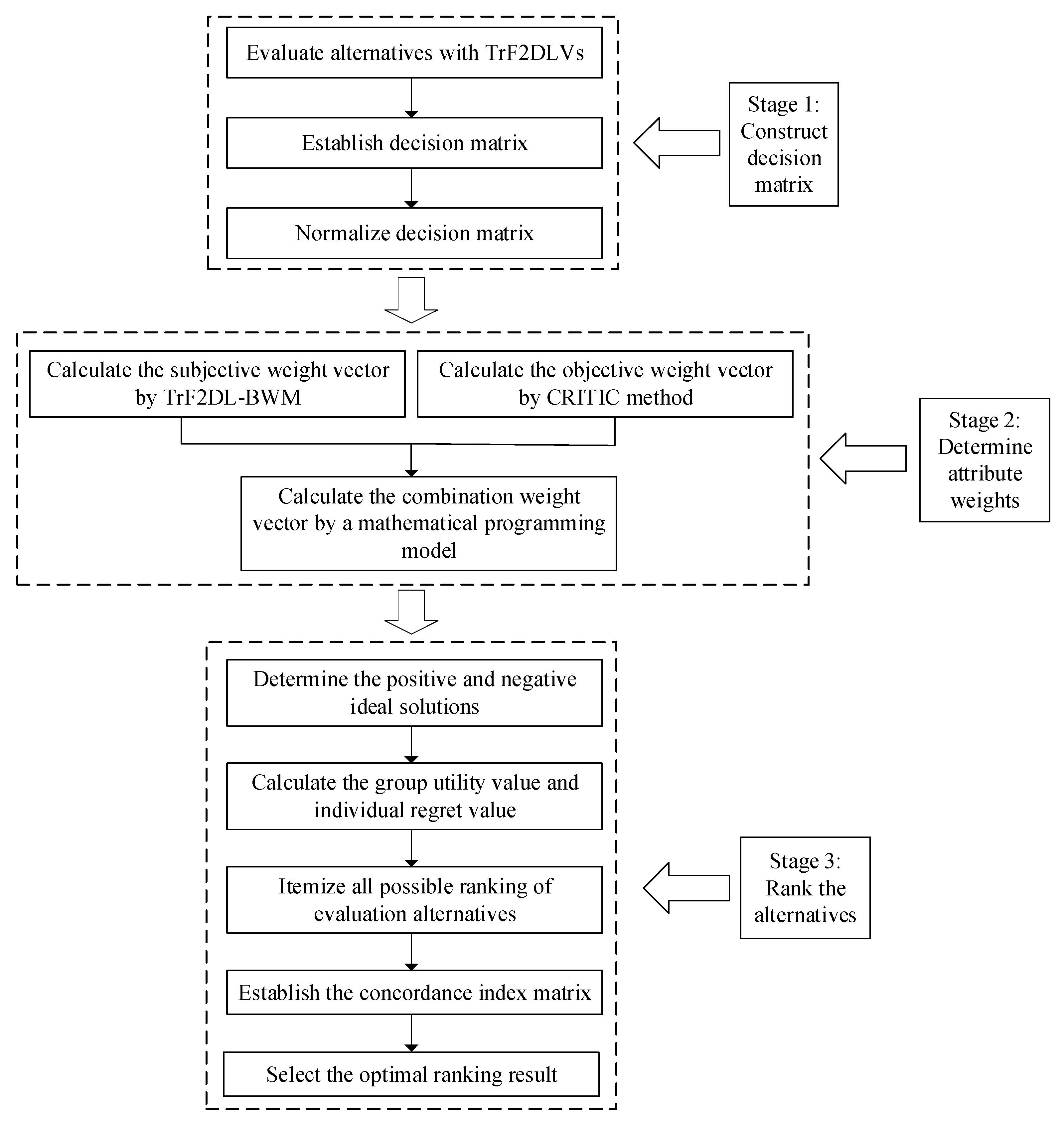
4. Extended VIKOR-QUALIFLEX Method Based on TrF2DLVs for MADM with Unknown Attribute Weight

4.1. Problem Description of MADM with Unknown Attribute Weight

It is assumed that the DMs need to rank the m alternatives $\left\{P_1,P_2,\dots ,P_m,\right\}$ for decision-making, in order to consider the alternatives comprehensively, n evaluation attributes $\left\{A_1,A_2,\dots ,A_n,\right\}$ are selected. To express the information accurately, the evaluation information is represented by TrF2DLVs. In addition, the attribute weights of the MADM problem are unknown, which need to be obtained through expert experience and evaluation information.

4.2. Extended VIKOR-QUALIFLEX Method Based on TrF2DLVs

To solve above MADM problems, an extended VIKOR-QUALIFLEX method based on trapezoidal fuzzy two-dimensional linguistic information is established in this section. This method is mainly divided into three stages, including obtaining evaluation information, obtaining attribute weight, and ranking alternatives. In stage 1, the DM try to use TrF2DLVs to evaluate alternatives based on different attributes and gives an evaluation matrix $X={\left[{\chi }_{ij}\right]}_{m\times n}$. In stage 2, in order to obtain unknown attribute weight, a weight determination model is constructed. It mainly includes three parts: (1) the TrF2DL-BWM is employed to calculate the subjective weight vector, (2) the CRITIC method is employed to calculate the objective weight vector, and (3) calculate the combination weight vector. In stage 3, the QUALIFLEX method is employed to rank the alternatives, in which a VIKOR method is employed to measure the concordance index of alternatives for pairwise comparison based on the weighted evaluation information. The specific steps of this decision method are as follows:

Step 1

Establish decision matrix $X={\left[{\chi }_{ij}\right]}_{m\times n}\left(i=1,2,\cdots ,m;j=1,2,\cdots ,n\right)$, where ${\chi }_{ij}$ is the evaluation value of the $i\mathrm{th}$ alternative according to the $j \mathrm{th}$ attribute represented by a TrF2DLV ${\chi }_{ij}=\left(\left[t_{ij}^L,t_{ij}^{ML},t_{ij}^{MU},t_{ij}^U\right],s_{{\epsilon }_{ij}}\right)$$\left(i=1,2,\dots ,m,j=1,2,\dots ,n\right)$. Then, normalize the decision-making unit ${\chi }_{ij}$ according to the attribute of benefit type or cost type. The normalized matrix $\tilde{X}={\left[{\tilde{\chi }}_{ij}\right]}_{m\times n}$ can be obtained from Equations (29) and (30) in Section 3.2.

Step 2

Calculate the weight vector of attributes using the weight determination model.

Step 2.1

Calculate the subjective weight vector $w={\left(w_1,w_2,\cdots w_n\right)}^T$ using TrF2DL-BWM in Section 2.1, where $0\le w_j\le 1$,${\displaystyle \sum _{j=1}^n{w}_j}=1$;

Step 2.2

Calculate the objective weight vector $\omega ={\left({\omega }_1,{\omega }_2,\cdots ,{\omega }_n\right)}^T$ using the CRITIC method in Section 2.2, where $0\le {\omega }_j\le 1$, ${\displaystyle \sum _{j=1}^n{\omega }_j}=1$;

Step 2.3

Calculate the combination weight vector $\varpi ={\left({\varpi }_1,{\varpi }_2,\cdots ,{\varpi }_n\right)}^T$ by a mathematical programming model in Section 2.3, where $0\le {\varpi }_j\le 1$, ${\displaystyle \sum _{j=1}^n{\varpi }_j}=1$.

Note: If the experts have enough information and knowledge reserves when acquiring the subjective weight, the proposed decision-making method can be further simplified, and the DMs may not need to calculate the objective weights and combination weights.

Step 3

Determine positive and negative ideal solutions of each subattribute.

The positive ideal solution ${\chi }_j^{+}=\underset{i}{\max }{\chi }_{ij}$ and the negative ideal solution ${\chi }_j^{-}=\underset{i}{\min }{\tilde{\chi }}_{ij}$.

Note: the comparison rules of ${\tilde{\chi }}_{ij}$ are described in Section 2.3.

Step 4

Calculate the group utility value $S_i\left(i=1,2,\cdots ,m\right)$ and individual regret value ${\mathsf{\Omega }}_i\left(i=1,2,\cdots ,m\right)$ of each evaluation alternative, where

$$S_i={\displaystyle \sum _{j=1}^n\frac{{\varpi }_j\times d\left({\chi }_j^{+},{\chi }_{ij}\right)}{d\left({\chi }_j^{+},{\chi }_j^{-}\right)}}\left(i=1,2,\cdots ,m\right)$$

(41)

$${\mathsf{\Omega }}_i=\underset{j}{\max }\left\{\frac{{\varpi }_{j}d\left({\chi }_j^{+},{\chi }_{ij}\right)}{d\left({\chi }_j^{+},{\chi }_j^{-}\right)}\right\}\left(i=1,2,\cdots ,m;j=1,2,\cdots ,n\right).$$

(42)

Step 5

List all possible ranking of m evaluation alternatives ${ℝ}_{\lambda }\left(\lambda =1,2,\cdots ,m!\right)$.

Step 6

The alternatives in each possible permutation ${ℝ}_{\lambda }$ are compared in pairs in order, and the concordance index $I_{ik}\left(i,k=1,2,\cdots ,m\right)$ of each comparison ($A_i\left(i=1,2,\cdots ,m\right)$ over $A_k\left(k=1,2,\cdots ,m\right)$) is calculated by the following Equation (43). Then, the concordance index matrix $I={\left[I_{ik}\right]}_{m\times m}\left(i,k=1,2,\cdots ,m\right)$ is established.

$$I_{ik}=\phi \frac{S_k-S_i}{S_{}^{+}-S^{-}}+\left(1-\phi \right)\frac{{\mathsf{\Omega }}_k-{\mathsf{\Omega }}_i}{{\mathsf{\Omega }}^{+}-{\mathsf{\Omega }}^{-}}\left(i,k=1,2,\cdots ,m\right),$$

(43)

where $S^{+}=\underset{i}{\min }\left\{S_i\right\}$, $S^{-}=\underset{i}{\max }\left\{S_i\right\}$, ${\mathsf{\Omega }}^{+}=\underset{i}{\min }\left\{{\mathsf{\Omega }}_i\right\}$, and ${\mathsf{\Omega }}^{-}=\underset{i}{\max }\left\{{\mathsf{\Omega }}_i\right\}$. $\phi$ is the decision-making mechanism coefficient, which can balance the weights between group utility and individual regret. When $\phi >0.5$, it indicates that DMs prefer to maximize group utility; when $\phi <0.5$, it indicates that DMs prefer to minimize individual regret. In this study, we suppose that the “the maximum group utility” and “minimum individual regret” have the same importance, that is, $\phi =0.5$.

Step 7

Calculate the overall concordance index $I^{{ℝ}_{\lambda }}$ for each possible ranking ${ℝ}_{\lambda }\left(\lambda =1,2,\cdots ,m!\right)$.

$$I^{{ℝ}_{\lambda }}={\displaystyle \sum _{i=1}^{m!-1}{\displaystyle \sum _{k=i+1}^{m!}{I}_{ik}}}\left(\lambda =1,2,\cdots ,m!\right)$$

(44)

Step 8

The ranking with the largest overall concordance index is selected as the final ranking result.

The process of the proposed method can be described by Figure 1.

5. Practical Case Application

Industrialized residential project is the trend of housing construction in the future, but the current project management system matching with the construction mode of industrialized residential project is relatively backward. It is urgent to create a management system and evaluation method suitable for the construction of industrialized residential projects, so as to give full play to the advantages of industrialized residential project. A research institute in China is ready to evaluate the lean management level of industrialized residential project in M city. Based on the previous literature review, expert interviews, and questionnaire survey, combined with the scientific principle, goal oriented principle, comparability principle, systematic principle, operability principle, and independence principle of index system construction, this research institute has determined the following evaluation index system for lean management of industrialized residential project. This index system is mainly developed from two levels: project process level and organization level. Based on the project process level, three primary attributes are determined, which are design lean management, component production and logistics lean management, and construction lean management. Based on the organization level, two primary attributes are determined, namely, organizational collaborative lean management and information collaborative lean management. In addition, each primary attribute is subdivided into multiple subattributes. The specific evaluation attribute system of lean management level of industrialized residential project is shown in

Table 1. Evaluation attribute system.

Primary Attributes	Subattributes
Design lean management A	Assembling design management A1
	Standardized design management A2
	Personalized design management A3
	Design suitability management A4
Component production and logistics lean management B	Component production standardization management B1
	Component quality control management B2
	Logistics time management B3
	Component lossless transport management B4
Construction lean management C	Construction mechanization management C1
	Environmental construction management C2
	Construction process management C3
	Construction safety management C4
Organizational collaborative lean management D	Organizational integration management D1
	Organizational trust management D2
	Cooperative intention management D3
	Organizational collaboration technology management D4
Information collaborative lean management E	Information accuracy management E1
	Information delivery time management E2
	Information transfer cost management E3

. Note: this index system has been tested by questionnaire, reliability and validity, exploratory factor analysis, and confirmatory factor analysis, which has been proved that it has good applicability. Due to the space limitation, this paper does not introduce the process and results of the test and analysis.

With the strong support of leaders and peers, this study selected three industrialized residential projects (P₁, P₂, and P₃) as the alternatives of this quantitative analysis. Note: P₁, P₂, and P₃ are now officially completed. As the content of the project involves many professional terms, in order not to affect the readability of the article, the specific content of each project is not detailed here. In this evaluation study, several experts who have participated in (or understood) the above three projects were selected as the main DMs, and lean management evaluation data of the three projects were obtained by on-site questionnaire scoring. The TrF2DLVs ${\chi }_{ij}^{\kappa }=\left(\left[t_{ij,\kappa }^L,t_{ij,\kappa }^{ML},t_{ij,\kappa }^{MU},t_{ij,\kappa }^U\right],s_{{\epsilon }_{ij,\kappa }}\right)$ $\left(i=1,2,\dots ,m,j=1,2,\dots ,n,\kappa =A,B,\dots ,E\right)$ are employed to evaluate the three projects. It should be noted that DMs use the LTS $\left\{s_0,s_1,s_2,s_3,s_4\right\}$ with five LTs to express the subjective trust in the second dimension of TrF2DLVs. In addition, for the trapezoidal fuzzy numbers in the first dimension of TrF2DLVs, they mainly come from the transformation of linguistic terms based on the reference [41]. The DMs use the information form of linguistic terms to express the evaluation information of the first dimension, and then, they are transformed into trapezoidal fuzzy numbers based on the relevant transformation rules in [41]. After the data preprocessing, the following evaluation matrix $X={\left[{\chi }_{ij}^{\kappa }\right]}_{m\times n}$ is obtained in

Table 2. Decision matrix $X$ based on trapezoid fuzzy two-dimensional linguistic variables (TrF2DLVs).

	${\mathit{P}}_1$	${\mathit{P}}_2$	${\mathit{P}}_3$
$A_1^{}$	([0.245, 0.267, 0.298, 0.321],$s_3$)	([0.256, 0.276, 0.281, 0.285],$s_3$)	([0.203, 0.237, 0.271, 0.305],$s_4$)
$A_2^{}$	([0.305, 0.343, 0.381, 0.419],$s_3$)	([0.312, 0.343, 0.365, 0.392],$s_3$)	([0.076, 0.114, 0.153, 0.191],$s_4$)
$A_3^{}$	([0.276, 0.322, 0.368, 0.414],$s_3$)	([0.356, 0.367, 0.373, 0.401],$s_3$)	([0.184, 0.230, 0.276, 0.322],$s_4$)
$A_4^{}$	([0.309, 0.347, 0.386, 0.425],$s_3$)	([0.398, 0.401, 0.412, 0.433],$s_3$)	([0.155, 0.193, 0.231, 0.270],$s_4$)
$B_1^{}$	([0.175, 0.219, 0.263, 0.307],$s_4$)	([0.350, 0.394, 0.438, 0.482],$s_2$)	([0.175, 0.219, 0.263, 0.307],$s_3$)
$B_2^{}$	([0.345, 0.389, 0.432, 0.475],$s_4$)	([0.234, 0.245, 0.259, 0.302],$s_2$)	([0.086, 0.130, 0.173, 0.216],$s_3$)
$B_3^{}$	([0.253, 0.284, 0.316, 0.348],$s_4$)	([0.312, 0.334, 0.345, 0.356],$s_2$)	([0.253, 0.284, 0.316, 0.348],$s_3$)
$B_4^{}$	([0.231, 0.270, 0.309, 0.347],$s_4$)	([0.356, 0.367, 0.381, 0.392],$s_2$)	([0.309, 0.347, 0.386, 0.424],$s_3$)
$C_1^{}$	([0.305, 0.343, 0.381, 0.419],$s_3$)	([0.305, 0.343, 0.381, 0.419],$s_4$)	([0.076, 0.114, 0.153, 0.191],$s_3$)
$C_2^{}$	([0.277, 0.312, 0.346, 0.381],$s_3$)	([0.346, 0.381, 0.381, 0.381],$s_4$)	([0.139, 0.173, 0.208, 0.242],$s_3$)
$C_3^{}$	([0.162, 0.203, 0.243, 0.284],$s_3$)	([0.162, 0.203, 0.243, 0.284],$s_4$)	([0.324, 0.365, 0.405, 0.446],$s_3$)
$C_4^{}$	([0.276, 0.322, 0.368, 0.414],$s_3$)	([0.184, 0.230, 0.276, 0.322],$s_4$)	([0.184, 0.230, 0.276, 0.322],$s_3$)
$D_1^{}$	([0.222, 0.259, 0.296, 0.333],$s_2$)	([0.296, 0.333, 0.370, 0.408],$s_3$)	([0.222, 0.259, 0.296, 0.333],$s_3$)
$D_2^{}$	([0.253, 0.284, 0.316, 0.348],$s_2$)	([0.253, 0.284, 0.316, 0.348],$s_3$)	([0.253, 0.284, 0.316, 0.348],$s_3$)
$D_3^{}$	([0.250, 0.313, 0.374, 0.437],$s_2$)	([0.250, 0.313, 0.374, 0.437],$s_3$)	([0.116, 0.174, 0.233, 0.291],$s_3$)
$D_4^{}$	([0.324, 0.365, 0.405, 0.446],$s_2$)	([0.162, 0.203, 0.243, 0.284],$s_3$)	([0.162, 0.203, 0.243, 0.284],$s_3$)
$E_1^{}$	([0.198, 0.248, 0.296, 0.346],$s_3$)	([0.245, 0.286, 0.327, 0.367],$s_3$)	([0.010, 0.050, 0.099, 0.149],$s_2$)
$E_2^{}$	([0.327, 0.367, 0.408, 0.449],$s_3$)	([0.209, 0.261, 0.312, 0.365],$s_3$)	([0.082,0.123,0.164,0.204],$s_2$)
$E_3^{}$	([0.364, 0.455, 0.545, 0.636],$s_3$)	([0.395, 0.445, 0.494, 0.544],$s_3$)	([0.209, 0.261, 0.312, 0.365],$s_2$)

.

5.1. Method Implementation Process

To solve the above practical application case through the proposed method, the specific steps are as follows:

Step 1.

Since all attribute types are benefit type, the normalization can be omitted.

Step 2.1.

Calculate the subjective weight vector $w={\left(w_1,w_2,\cdots w_{19}\right)}^T$ using TrF2DL-BWM.

Step 2.1.1.

First, the best attribute and the worst attribute are determined among all the primary attributes. Then, the best attribute and the worst attribute among the subattributes of each primary attribute are determined.

For the five primary attributes, the DMs determine that the best attribute is $A$ and the worst attribute is $E$. For the four subattributes under the primary attribute $A$, DMs determine that the best attribute is $A_1^{}$, and the worst subattribute is $A_3^{}$. Similarly, for other primary attributes, the best subattributes are $B_1^{}$, $C_4^{}$, $D_1^{}$, and $E_1^{}1$, and the worst subattributes are $B_4^{}$, $C_3^{}$, $D_3^{}$, and $E_3^{}$.

Step 2.1.2.

For the five primary attributes, DMs give the Best-to-Others vector:

${\chi }_{best}$ = ${\chi }_A=\{{\chi }_{A,A},{\chi }_{A,B},{\chi }_{A,C},{\chi }_{A,D},{\chi }_{A,E}\}$ = {([0.500, 0.500, 0.500, 0.500],$s_4$), ([0.667, 0.733, 0.800, 0.867],$s_4$), ([0.533, 0.600, 0.667, 0.733],$s_4$), ([0.733, 0.800, 0.867, 0.933],$s_4$), ([0.800, 0.867, 0.933, 1.000],$s_4$)}, and the Others-to-Worst vector:

${\chi }_{worst}$ = ${\chi }_E=\{{\chi }_{A,E},{\chi }_{B,E},{\chi }_{C,E},{\chi }_{D,E},{\chi }_{E,E}\}$ = {([0.800, 0.867, 0.933, 1.000],$s_4$), ([0.533, 0.600, 0.667, 0.733],$s_4$), ([0.667, 0.733, 0.800, 0.867],$s_4$), ([0.667, 0.733, 0.800, 0.867],$s_3$), ([0.500, 0.500, 0.500, 0.500],$s_4$)}.

For the four subattributes under the primary attribute $A$, DMs give the Best-to-Others vector:

${\chi }_{best}^A$ = ${\chi }_1^A=\{{\chi }_{1,1}^A,{\chi }_{1,2}^A,{\chi }_{1,3}^A,{\chi }_{1,4}^A\}$ = {([0.500, 0.500, 0.500, 0.500],$s_4$), ([0.533, 0.600, 0.667, 0.733],$s_4$), ([0.800, 0.867, 0.933, 1.000],$s_4$), ([0.667, 0.733, 0.800, 0.867],$s_4$)}, and the Others-to-Worst vector:

${\chi }_{worst}^A$$={\chi }_3^A=\{{\chi }_{1,3}^A,{\chi }_{2,3}^A,{\chi }_{3,3}^A,{\chi }_{4,3}^A\}$ = {([0.800, 0.867, 0.933, 1.000],$s_4$), ([0.667, 0.733, 0.800, 0.867],$s_4$), ([0.500, 0.500, 0.500, 0.500],$s_4$), ([0.667, 0.733, 0.800, 0.867],$s_3$)}.

Similarly, DMs can give the Best-to-Others vectors and the Others-to-Worst vectors of other subattributes under the primary attribute $B$, $C$, $D$, and $E$. For the convenience of reading, they are omitted here.

Step 2.1.3.

Convert the vector ${\chi }_{best}$ and ${\chi }_{worst}$ to $e_{best}$ and $e_{worst}$, respectively.

Here, we only take the primary attributes as an example to give the experimental results. $e_{best}$ = $e_A=\{e_{A,A},e_{A,B},e_{A,C},e_{A,D},e_{A,E}\}$ = {0.500, 0.767, 0.633, 0.833, 0.930},

$e_{worst}=e_E=$$\{e_{A,E},e_{B,E},e_{C,E},e_{D,E},$$e_{E,E}\}$ = {0.900, 0.633, 0.767, 0.575,0.500}.

Step 2.1.4.

For the five primary attributes, we can build the following model based on Equation (28):

$\min \hspace{0.17em}{\delta }^{\ast }$

$$\begin{array}{c}St.\\ \left|\frac{5-1}{2}(w_A-w_A)+0.5-e_{A,A}\right|\le {\delta }^{\ast };\left|\frac{5-1}{2}(w_A-w_B)+0.5-e_{A,B}\right|\le {\delta }^{\ast }; \\ \left|\frac{5-1}{2}(w_A-w_C)+0.5-e_{A,C}\right|\le {\delta }^{\ast };\\ \left|\frac{5-1}{2}(w_A-w_D)+0.5-e_{A,D}\right|\le {\delta }^{\ast }; \left|\frac{5-1}{2}(w_A-w_E)+0.5-e_{A,E}\right|\le {\delta }^{\ast }; \\ \left|\frac{5-1}{2}(w_A-w_E)+0.5-e_{A,E}\right|\le {\delta }^{\ast };\\ \left|\frac{5-1}{2}(w_B-w_E)+0.5-e_{B,E}\right|\le {\delta }^{\ast }; \left|\frac{5-1}{2}(w_C-w_E)+0.5-e_{C,E}\right|\le {\delta }^{\ast }; \\ \left|\frac{5-1}{2}(w_D-w_E)+0.5-e_{D,E}\right|\le {\delta }^{\ast };\\ \left|\frac{5-1}{2}(w_E-w_E)+0.5-e_{E,E}\right|\le {\delta }^{\ast }; {\displaystyle \sum _{j=A}^E{w}_j}=1; {\delta }^{\ast }\ge 0,\hspace{0.17em}{w}_j\ge 0,\hspace{0.17em}j=A,B,\dots ,E.\end{array}$$

We employ the LINGO to solve above model and obtain the subjective weight vector $w^{*}={(0.314,0.179,0.246,0.149,0.113)}^T$ and ${\delta }^{\ast }$ = 0.003. Similarly, we have the other weight vectors $w_A$ = (0.380, 0.304, 0.126, 0.189)^T, $w_B$ = (0.386, 0.282, 0.216, 0.116)^T, $w_C$ = (0.240, 0.283,0.135,0.342)^T, $w_D$ = (0.387, 0.313, 0.106, 0.194)^T, and $w_E$ = (0.403, 0.64, 0.233)^T and ${\delta }_A^{*}$ = 0.019, ${\delta }_B^{*}$ = 0.018, ${\delta }_C^{*}$ = 0.022, ${\delta }_D^{*}$ = 0.022, and ${\delta }_E^{*}$ = 0.006.

It is easy to find that the value of objective function ${\delta }_{\kappa }^{*}(\kappa =A,B\dots ,E)$ are very close to 0, so the obtained subjective weights have high reliability.

To obtain the global subjective weights for each subattribute, the subjective weights of corresponding main attribute need be multiplied by the local subjective weights of each subattribute. Thus, we can obtain the global subjective weight vector of all subattributes:

w = (0.119, 0.095, 0.040, 0.059, 0.069, 0.050, 0.039, 0.021, 0.059, 0.070, 0.033, 0.084, 0.058, 0.047, 0.016, 0.029, 0.045, 0.041, 0.026)^T.

Step 2.2.

Calculate the objective weight vector $\omega ={\left({\omega }_1,{\omega }_2,\cdots ,{\omega }_{19}\right)}^T$ using the CRITIC method in Section 2.2.

Step 2.2.1.

For the four subattributes under the primary attribute $A$, we calculate the correlation coefficient ${\rho }_{{}_{jl}}^A$ (j, l = 1, 2, 3, 4) between the jth and the lth attributes by the Equations (31) and (32), and the following correlation coefficient matrix: ${\rho }^A={\left[{\rho }_{{}_{jl}}^A\right]}_{4\times 4}$ can be determined:

$$\begin{array}{l}\hspace{1em}\hspace{1em}\hspace{1em}\hspace{1em}\hspace{1em}{A}_1\hspace{1em}\hspace{0.17em}\hspace{0.17em}{A}_2\hspace{1em}\hspace{0.17em}\hspace{0.17em}{A}_3\hspace{1em}\hspace{0.17em}\hspace{0.17em}{A}_4\\ {\rho }^A=\begin{array}{c}{A}_1\\ A_2\\ A_3\\ A_4\end{array}\left[\begin{array}{cccc}1& 0.814& 0.352& 0.571\\ 0.814& 1& 0.788& 0.902\\ 0.352& 0.788& 1& 0.969\\ 0.571& 0.902& 0.969& 1\end{array}\right].\end{array}$$

Similarly, the other correlation coefficient matrices can be obtained:

$$\begin{gathered} \begin{array}{l}\hspace{1em}\hspace{1em}\hspace{1em}\hspace{1em}\hspace{1em}{B}_1\hspace{1em}\hspace{0.17em}\hspace{0.17em}{B}_2\hspace{1em}\hspace{0.17em}\hspace{0.17em}{B}_3\hspace{1em}\hspace{0.17em}\hspace{0.17em}{B}_4\\ {\rho }^B=\begin{array}{c}{B}_1\\ B_2\\ B_3\\ B_4\end{array}\left[\begin{array}{cccc}1& 0.844& 0.887& 0.838\\ 0.844& 1& 0.934& 0.804\\ 0.887& 0.934& 1& 0.963\\ 0.838& 0.804& 0.963& 1\end{array}\right], \end{array}\begin{array}{l}\hspace{1em}\hspace{1em}\hspace{1em}\hspace{1em}\hspace{0.17em}\hspace{0.17em}{C}_1\hspace{1em}\hspace{1em}{C}_2\hspace{1em}\hspace{1em}{C}_3\hspace{1em}\hspace{0.17em}{C}_4\\ {\rho }^C=\begin{array}{c}{C}_1\\ C_2\\ C_3\\ C_4\end{array}\left[\begin{array}{cccc}1& 0.975& 0.771& 0.878\\ 0.975& 1& 0.619& 0.801\\ 0.771& 0.619& 1& 0.724\\ 0.878& 0.801& 0.724& 1\end{array}\right]\end{array} \\ \begin{array}{l}\hspace{1em}\hspace{1em}\hspace{1em}\hspace{1em}\hspace{1em}{D}_1\hspace{1em}\hspace{0.17em}\hspace{0.17em}{D}_2\hspace{1em}\hspace{0.17em}\hspace{0.17em}{D}_3\hspace{1em}\hspace{0.17em}\hspace{0.17em}{D}_4\\ {\rho }^D=\begin{array}{c}{D}_1\\ D_2\\ D_3\\ D_4\end{array}\left[\begin{array}{cccc}1& 0.946& 0.905& 0.647\\ 0.946& 1& 0.718& 0.602\\ 0.905& 0.718& 1& 0.598\\ 0.647& 0.602& 0.598& 1\end{array}\right], \end{array}\begin{array}{l}\hspace{1em}\hspace{1em}\hspace{1em}\hspace{1em}\hspace{0.17em}\hspace{0.17em}{E}_1\hspace{1em}\hspace{1em}{E}_2\hspace{1em}\hspace{0.17em}\hspace{0.17em}{E}_3\\ {\rho }^E=\begin{array}{c}{E}_1\\ E_2\\ E_3\end{array}\left[\begin{array}{ccc}1& 0.903& 0.974\\ 0.903& 1& 0.964\\ 0.974& 0.964& 1\end{array}\right]\end{array} \end{gathered}$$

For the correlation coefficient matrix of primary attributes, we first aggregate the subattributes under each primary attribute for each alternative using the following Equation (45).

$${\chi }_i^{\kappa }=⟮\frac{1}{n}\left[{\displaystyle \sum _{j=1}^n{t}_{ij,\kappa }^L},{\displaystyle \sum _{j=1}^n{t}_{ij,\kappa }^{ML}},{\displaystyle \sum _{j=1}^n{t}_{ij,\kappa }^{MU}},{\displaystyle \sum _{j=1}^n{t}_{ij,\kappa }^U}\right],s_{\min ({\epsilon }_{ij,\kappa }^{})}⟯;\kappa =A,B,C,D,E.$$

(45)

Then, we obtain the following matrix $\rho ={\left[{\rho }_{{}_{jl}}^{}\right]}_{5\times 5}(j,l=A,B,C,D,E)$ using the similar method mentioned above.

$$\begin{array}{l}\hspace{1em}\hspace{1em}\hspace{1em}\hspace{1em}A\hspace{1em}\hspace{1em}B\hspace{1em}\hspace{1em}C\hspace{1em}\hspace{1em}D\hspace{1em}\hspace{1em}E\\ \rho =\begin{array}{c}A\\ B\\ C\\ D\\ E\end{array}\left[\begin{array}{ccccc}1& 0.707& 0.929& 0.903& 0.965\\ 0.707& 1& 0.418& 0.395& 0.863\\ 0.929& 0.418& 1& 0.994& 0.820\\ 0.903& 0.395& 0.994& 1& 0.799\\ 0.965& 0.863& 0.820& 0.799& 1\end{array}\right]\end{array}$$

Step 2.2.3.

For the primary attributes, calculate the standard deviation ${\sigma }_j$ of the $j\mathrm{th}$ (j = A, B, C, D, E) primary attribute by Equation (33). Similarly, the standard deviation ${\sigma }_j^{\kappa }$ (j = 1, 2, 3, 4 when $\kappa =A,B,C,D$ and j = 1, 2, 3 when $\kappa =E$) of subattributes under each primary attribute can also be obtained.

$$\begin{gathered} {\sigma }_1^A=0.030,{\sigma }_2^A=0.064,{\sigma }_3^A=0.024,{\sigma }_4^A=0.044; \\ {\sigma }_1^B=0.065,{\sigma }_2^B=0.158,{\sigma }_3^B=0.092,{\sigma }_4^B=0.091; \\ {\sigma }_1^C=0.113,{\sigma }_2^C=0.099,{\sigma }_3^C=0.053,{\sigma }_4^C=0.038; \\ {\sigma }_1^D=0.073,{\sigma }_2^D=0.061,{\sigma }_3^D=0.065,{\sigma }_4^D=0.039; \\ {\sigma }_1^E=0.097,{\sigma }_2^E=0.106,{\sigma }_3^E=0.132, \\ {\sigma }_A=0.029,{\sigma }_B=0.153,{\sigma }_C=0.047,{\sigma }_D=0.049,{\sigma }_E=0.061. \end{gathered}$$

Step 2.2.4.

According to Equations (34) and (35), the objective weight vector ${\omega }^{*}={\left({\omega }_A,{\omega }_B,\dots ,{\omega }_E\right)}^T$ for primary attributes and the objective weight vector ${\omega }_{\kappa }^{}={\left({\omega }_1,{\omega }_2,\dots ,{\omega }_n\right)}^T(\kappa =A,B,C,D,E)$ can be obtained as below:

$$\begin{gathered} {\omega }^{*} = (0.044, 0.473, 0.145, 0.150, 0.188),{\omega }_A = {(0.328, 0.276, 0.186, 0.209)}^T, \\ {\omega }_B = {(0.187, 0.441, 0.133, 0.239)}^T, {\omega }_C = {(0.247, 0.348, 0.274, 0.131)}^T, \\ {\omega }_D = {(0.208, 0.254, 0.284, 0.254)}^T, {\omega }_E = {(0.349, 0.412, 0.240)}^T. \end{gathered}$$

To obtain the global objective weights for each subattribute, the objective weights of corresponding main attribute need to be multiplied by the local objective weights of each subattribute. Thus, we can obtain the global objective weight vector of all subattributes:

ω = (0.014, 0.012, 0.008, 0.009, 0.089, 0.209, 0.063, 0.113, 0.036, 0.050, 0.040, 0.019, 0.031, 0.038, 0.043, 0.038, 0.066, 0.077, 0.045)^T.

Step 2.3.

Calculate the combination weight vector $\varpi ={\left({\varpi }_1,{\varpi }_2,\cdots ,{\varpi }_{19}\right)}^T$ of all subattributes by the mathematical programming model in Section 2.3 and Equation (40). The result is as follows:

ϖ = (0.092, 0.074, 0.032, 0.046, 0.074, 0.091, 0.045, 0.045, 0.053, 0.065, 0.035, 0.067, 0.051, 0.044, 0.023, 0.031, 0.051, 0.050, 0.031)^T.

Step 3.

Determine positive and negative ideal solutions of each subattribute.

$$\begin{gathered} {\chi }_1^{+} = \left\{\right([0.203, 0.237, 0.271, 0.305], s_4\left)\right\}, {\chi }_1^{-} = \left\{\right([0.256, 0.276, 0.281, 0.285], s_3\left)\right\}, \\ {\chi }_2^{+} = \left\{\right([0.305, 0.343, 0.381, 0.419], s_3\left)\right\}, {\chi }_2^{-} = \left\{\right([0.076, 0.114, 0.153, 0.191], s_4\left)\right\}, \\ {\chi }_3^{+} = \left\{\right([0.356, 0.367, 0.373, 0.401], s_3\left)\right\}, {\chi }_3^{-} = \left\{\right([0.184, 0.230, 0.276, 0.322], s_4\left)\right\}, \\ {\chi }_4^{+} = \left\{\right([0.398, 0.401, 0.412, 0.433], s_3\left)\right\}, {\chi }_4^{-} = \left\{\right([0.155, 0.193, 0.231, 0.270], s_4\left)\right\}, \\ {\chi }_5^{+} = \left\{\right([0.175, 0.219, 0.263, 0.307], s_4\left)\right\}, {\chi }_5^{-} = \left\{\right([0.175, 0.219, 0.263, 0.307], s_3\left)\right\}, \\ {\chi }_6^{+} = \left\{\right([0.345, 0.389, 0.432, 0.475], s_4\left)\right\}, {\chi }_6^{-} = \left\{\right([0.086, 0.130, 0.173, 0.216], s_3\left)\right\}, \\ {\chi }_7^{+} = \left\{\right([0.253, 0.284, 0.316, 0.348], s_4\left)\right\}, {\chi }_7^{-} = \left\{\right([0.312, 0.334, 0.345, 0.356], s_2\left)\right\}, \\ {\chi }_8^{+} = \left\{\right([0.231, 0.270, 0.309, 0.347], s_4\left)\right\}, {\chi }_8^{-} = \left\{\right([0.356, 0.367, 0.381, 0.392], s_2\left)\right\}, \\ {\chi }_9^{+} = \left\{\right([0.305, 0.343, 0.381, 0.419], s_4\left)\right\}, {\chi }_9^{-} = \left\{\right([0.076, 0.114, 0.153, 0.191], s_3\left)\right\}, \\ {\chi }_{10}^{+} = \left\{\right([0.346, 0.381,0.381, 0.381], s_4\left)\right\}, {\chi }_{10}^{-} = \left\{\right([0.139, 0.173, 0.208, 0.242], s_3\left)\right\}, \\ {\chi }_{11}^{+} = \left\{\right([0.324, 0.365, 0.405, 0.446], s_3\left)\right\}, {\chi }_{11}^{-} = \left\{\right([0.162, 0.203, 0.243, 0.284], s_3\left)\right\}, \\ {\chi }_{12}^{+} = \left\{\right([0.276, 0.322, 0.368, 0.414], s_3\left)\right\}, {\chi }_{12}^{-} = \left\{\right([0.184, 0.230, 0.276, 0.322], s_3\left)\right\}, \\ {\chi }_{13}^{+} = \left\{\right([0.296, 0.333, 0.370, 0.408], s_3\left)\right\}, {\chi }_{13}^{-} = \left\{\right([0.222, 0.259, 0.296, 0.333], s_2\left)\right\}, \\ {\chi }_{14}^{+} = \left\{\right([0.253, 0.284, 0.316, 0.348], s_3\left)\right\}, {\chi }_{14}^{-} = \left\{\right([0.253, 0.284, 0.316, 0.348], s_2\left)\right\}, \\ {\chi }_{15}^{+} = \left\{\right([0.250, 0.313, 0.374, 0.437], s_3\left)\right\}, {\chi }_{15}^{-} = \left\{\right([0.116, 0.174, 0.233, 0.291], s_3\left)\right\}, \\ {\chi }_{16}^{+} = \left\{\right([0.324, 0.365, 0.405, 0.446], s_2\left)\right\}, {\chi }_{16}^{-} = \left\{\right([0.162, 0.203, 0.243, 0.284], s_3\left)\right\}, \\ {\chi }_{17}^{+} = \left\{\right([0.245, 0.286, 0.327, 0.367], s_3\left)\right\}, {\chi }_{17}^{-} = \left\{\right([0.010, 0.050, 0.099, 0.149], s_2\left)\right\}, \\ {\chi }_{18}^{+} = \left\{\right([0.327, 0.367, 0.408, 0.449], s_3\left)\right\}, {\chi }_{18}^{-} = \left\{\right([0.082, 0.123, 0.164, 0.204] s_2\left)\right\}, \\ {\chi }_{19}^{+} = \left\{\right([0.364, 0.455, 0.545, 0.636], s_3\left)\right\}, {\chi }_{19}^{-} = \left\{\right([0.209, 0.261, 0.312, 0.365], s_2\left)\right\}. \end{gathered}$$

Step 4.

Calculate the group utility value $S_i\left(i=1,2,3\right)$ and individual regret value ${\mathsf{\Omega }}_i\left(i=1,2,3\right)$ of each evaluation alternative based on Equations (41) and (42),

$$S_1=0.330,S_2=0.390,S_3=0.743; {\mathsf{\Omega }}_1=0.080,{\mathsf{\Omega }}_2=0.092,{\mathsf{\Omega }}_3=0.091.$$

Step 5.

All possible ranking of 3 evaluation alternatives ${ℝ}_{\lambda }\left(\lambda =1,2,\cdots ,6\right)$ can be listed:

$${ℝ}_1=\left(1,2,3\right),{ℝ}_2=\left(1,3,2\right),{ℝ}_3=\left(2,1,3\right),{ℝ}_4=\left(2,3,1\right),{ℝ}_5=\left(3,1,2\right),{ℝ}_6=\left(3,2,1\right).$$

Step 6.

The concordance index matrix $I={\left[I_{ik}\right]}_{3\times 3}\left(i,k=1,2,3\right)$ is established by Equation (43),

$$I=\left[\begin{array}{ccc}0& 0.572& 0.952\\ -0.572& 0& 0.380\\ -0.952& -0.380& 0\end{array}\right].$$

Step 7.

Calculate the overall concordance index $I^{{ℝ}_{\lambda }}$ for each possible ranking ${ℝ}_{\lambda }$ by Equation (44),

$$I^{{ℝ}_1}=1.904,I^{{ℝ}_2}=1.145,I^{{ℝ}_3}=0.759,I^{{ℝ}_4}=-1.145,I^{{ℝ}_5}=-0.759,I^{{ℝ}_6}=-1.904.$$

Step 8.

The largest overall concordance index is $I^{{ℝ}_1}$, thus the ranking result is $P_1\succ P_2\succ P_3$.

Thus, the project $P_1$ has the best level of lean management.

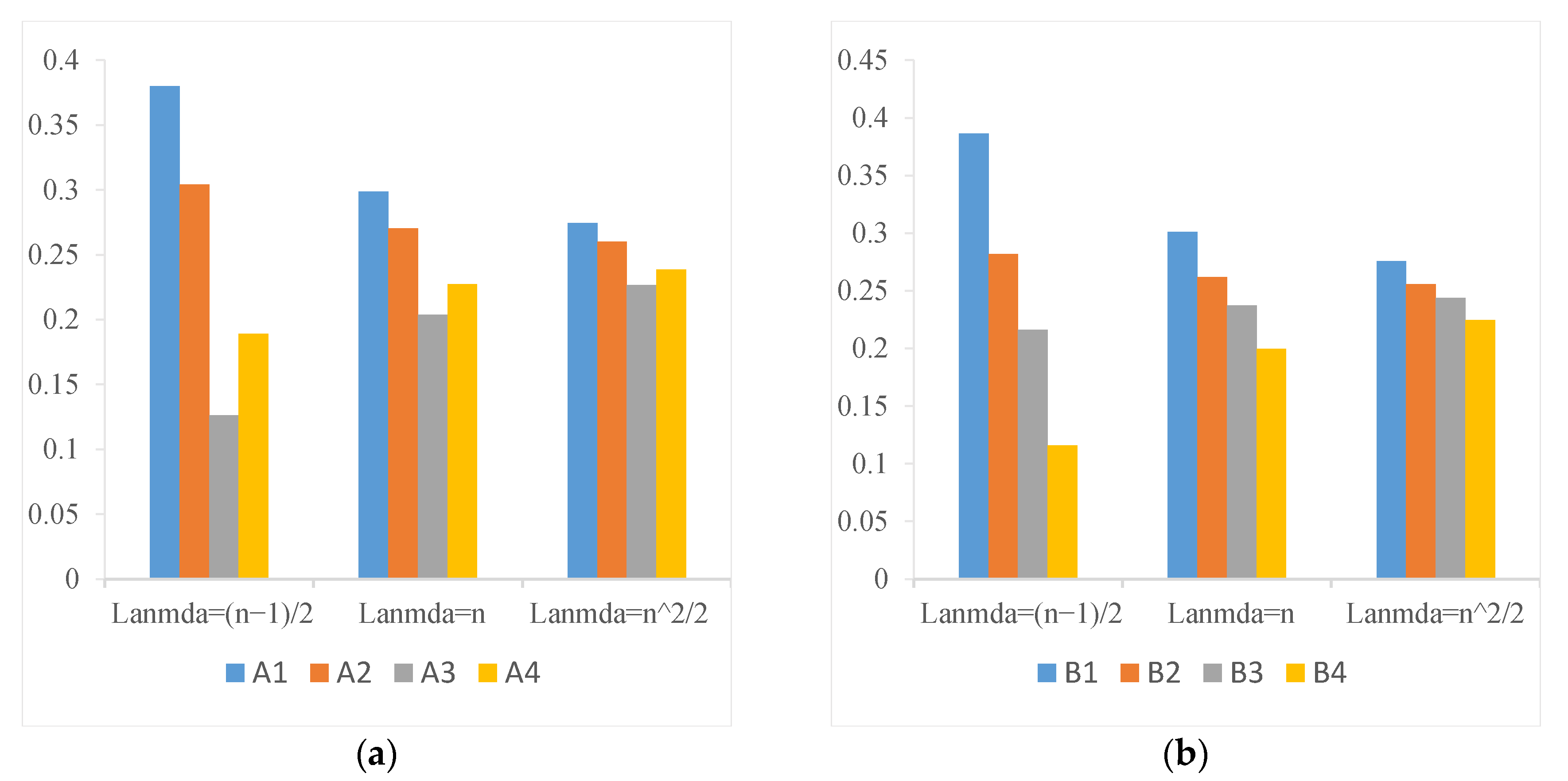
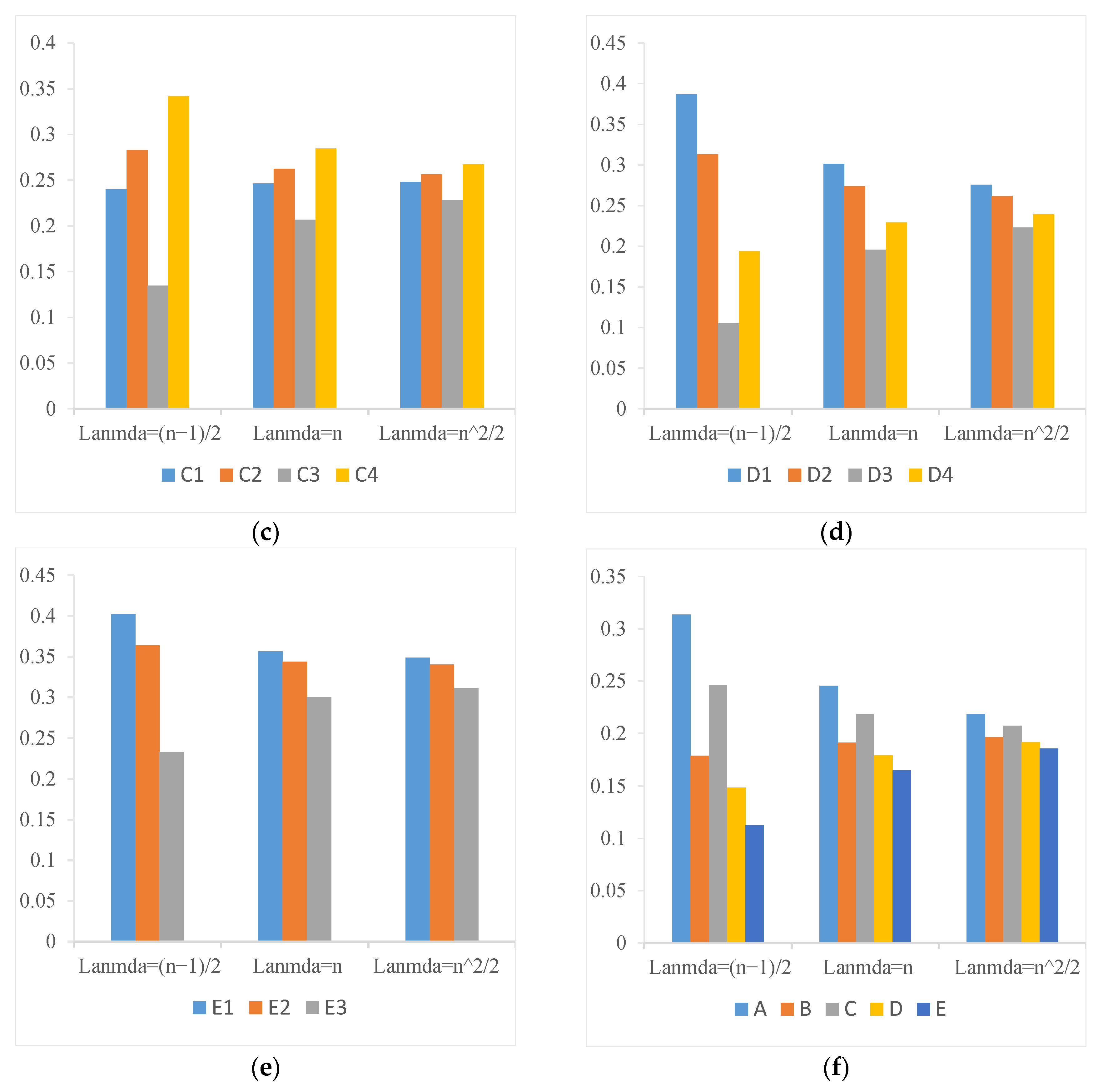
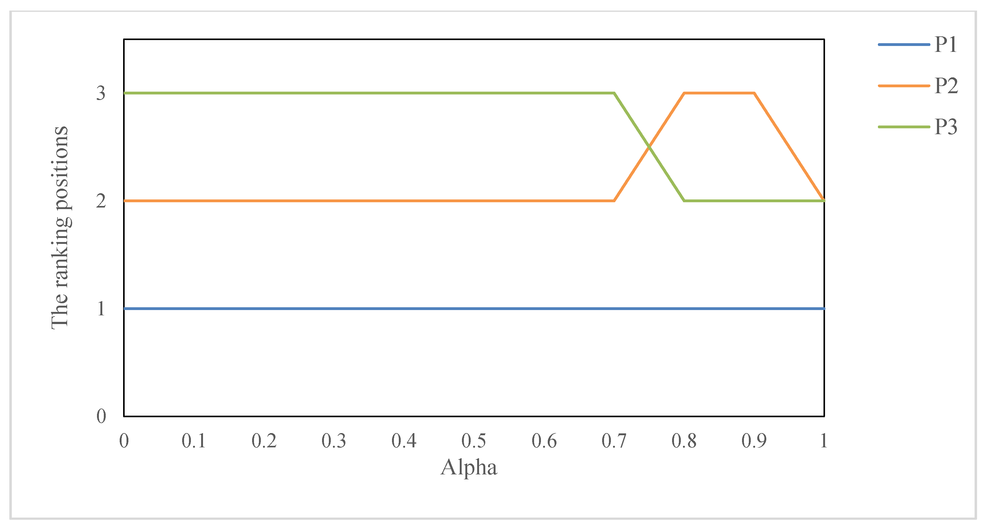
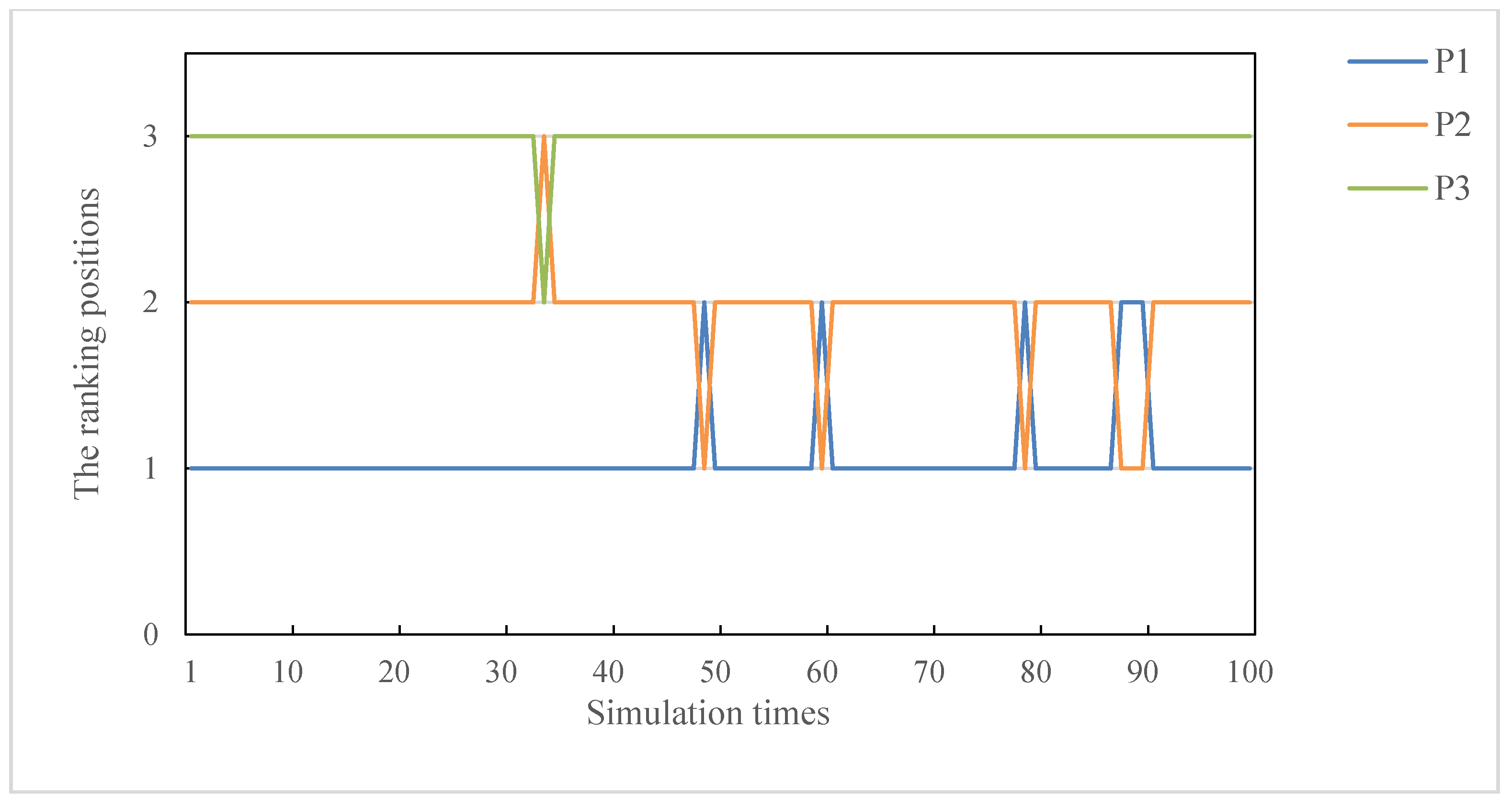
5.2. Parameter Sensitivity Analysis

The parameter $\lambda$ is involved in the method of obtaining subjective weight. Therefore, in this section, we will analyze the influence of different values of parameter $\lambda$ on subjective weight, combination weight, and ranking result. Let $\lambda =(n-1)/2$, $\lambda =n$, and $\lambda =n^2/2$ employ the method proposed in Section 3.1 to obtain local subjective weights of each subattribute and five primary attributes and then obtain global subjective weights of 19 subattributes. The experimental results are shown in Figure 2 and Figure 3. Then, let $\lambda =(n-1)/2$, $\lambda =n$, and $\lambda =n^2/2$ to obtain the combination weights of 19 subattributes by the method proposed in Section 3.1. The experimental results are shown in Figure 4. In addition, based on different values of $\lambda$, the ranking results are shown in

Table 3. Ranking obtained from different parameter $\lambda$.

$\mathit{\lambda }$	Weights	$\mathbf{Overall} \mathbf{Concordance} \mathbf{Index} {\mathit{I}}^{{\mathit{ℝ}}_1}$	Ranking
$\lambda =(n-1)/2$	Subjective weights	$\begin{array}{l}{I}^{{ℝ}_1}=0.570,I^{{ℝ}_2}=0.570,I^{{ℝ}_3}=0.000,I^{{ℝ}_4}=-0.570,I^{{ℝ}_5}=0.000,\\ I^{{ℝ}_6}=-0.570\end{array}$	$P_1\succ P_2=P_3$
	Combination weights	$\begin{array}{l}{I}^{{ℝ}_1}=1.904,I^{{ℝ}_2}=1.145,I^{{ℝ}_3}=0.759,I^{{ℝ}_4}=-1.145,I^{{ℝ}_5}=-0.759,\\ I^{{ℝ}_6}=-1.904\end{array}$	$P_1\succ P_2\succ P_3$
$\lambda =n$	Subjective weights	$\begin{array}{l}{I}^{{ℝ}_1}=1.209,I^{{ℝ}_2}=0.949,I^{{ℝ}_3}=0.260,I^{{ℝ}_4}=-0.949,I^{{ℝ}_5}=-0.260,\\ I^{{ℝ}_6}=-1.209\end{array}$	$P_1\succ P_2\succ P_3$
	Combination weights	$\begin{array}{l}{I}^{{ℝ}_1}=1.253,I^{{ℝ}_2}=1.006,I^{{ℝ}_3}=0.247,I^{{ℝ}_4}=-1.006,I^{{ℝ}_5}=-0.247,\\ I^{{ℝ}_6}=-1.253\end{array}$	$P_1\succ P_2\succ P_3$
$\lambda =n^2/2$	Subjective weights	$\begin{array}{l}{I}^{{ℝ}_1}=1.971,I^{{ℝ}_2}=0.555,I^{{ℝ}_3}=1.416,I^{{ℝ}_4}=-0.555,I^{{ℝ}_5}=-1.416,\\ I^{{ℝ}_6}=-1.971\end{array}$	$P_1\succ P_2\succ P_3$
	Combination weights	$\begin{array}{l}{I}^{{ℝ}_1}=1.985,I^{{ℝ}_2}=0.515,I^{{ℝ}_3}=1.470,I^{{ℝ}_4}=-0.515,I^{{ℝ}_5}=-1.470,\\ I^{{ℝ}_6}=-1.985\end{array}$	$P_1\succ P_2\succ P_3$

.

From Figure 2, it is easy to find that parameter $\lambda$ has obvious influence on local subjective weight of subattributes. When $\lambda =(n-1)/2$, the weight differentiation of each local attribute is obvious, but when $\lambda$ gradually increases ($\lambda =n$ and $\lambda =n^2/2$), the local weight difference of each subattribute decreases, which is close to each other in numerical value. However, it should be noted that regardless of the value of $\lambda$, the priority relationship of attributes at each level is unchanged. For example, for the five primary attributes, no matter what value $\lambda$ takes, the priority relationships of attribute weight are w_A > w_C >w_B> w_D >w_E. In addition, the larger the value of $\lambda$, the closer the distribution of attribute weight to uniform distribution. The smaller the parameter $\lambda$, the greater the gap between the weights. From Figure 3 and Figure 4, we can also find that the global weights of 19 subattributes are also affected by the value of $\lambda$. The smaller the $\lambda$ is, the more obvious the difference between attribute weights is, and the priority relationship between attributes is easier to distinguish. Besides, it can be seen from the results in Table 3, whether based on subjective weights or combined weights, parameter $\lambda$ has no effect on the ranking results from this case. From the analysis of additive consistency Formula (22), it can be found that when $\lambda$ is large enough, the weight gap between attribute i and attribute j can be small enough, but the priority relationship between the two attributes is fixed. Therefore, when $\lambda$ takes a smaller value, the sequence of attribute priority relation with more obvious discrimination can be obtained. In this case, we believe that the preference evaluation information is highly reliable. When $\lambda$ is large, the weight distribution of all attributes is balanced. In this case, the priority of attributes cannot be clearly distinguished. Therefore, parameter $\lambda$ can be flexibly applied to different index systems and DMs with different distinguishing ability. For example, parameter $\lambda$ should be set to a smaller value when the index system requires that each index has a more obvious discrimination. If the DMs thinks that there should be some fairness between attributes, then they can set a larger value of $\lambda$.

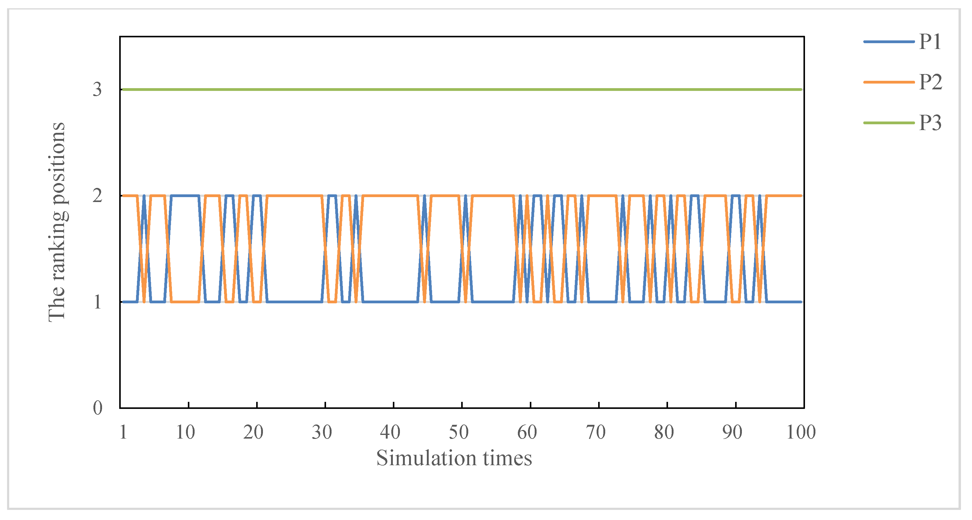
5.3. Weight Sensitivity Analysis

The core of this study is about the determination of attribute weight. We will analyze the impact of weight on the evaluation results. In the following table, we only use subjective weight and objective weight to deal with this evaluation problem. Using this proposed method, the ranking can be shown in

Table 4. Ranking obtained from different weights.

Weights	$\mathbf{Overall} \mathbf{Concordance} \mathbf{Index} {\mathit{I}}^{{\mathit{ℝ}}_1}$	Ranking
Subjective weights	$\begin{array}{l}{I}^{{ℝ}_1}=0.570,I^{{ℝ}_2}=0.570,I^{{ℝ}_3}=0.000,I^{{ℝ}_4}=-0.570,I^{{ℝ}_5}=0.000,\\ I^{{ℝ}_6}=-0.570\end{array}$	$P_1\succ P_2=P_3$
Objective weights	$\begin{array}{l}{I}^{{ℝ}_1}=2.000,I^{{ℝ}_2}=1.506,I^{{ℝ}_3}=0.494,I^{{ℝ}_4}=-1.506,I^{{ℝ}_5}=-0.494,\\ I^{{ℝ}_6}=-2.000\end{array}$	$P_1\succ P_2\succ P_3$
Combination weights	$\begin{array}{l}{I}^{{ℝ}_1}=1.904,I^{{ℝ}_2}=1.145,I^{{ℝ}_3}=0.759,I^{{ℝ}_4}=-1.145,I^{{ℝ}_5}=-0.759,\\ I^{{ℝ}_6}=-1.904\end{array}$	$P_1\succ P_2\succ P_3$

.

It is easy to find from Table 4 that when only the objective attribute weights are used, the ranking results are the same as that of the combination attribute weights, however, when only subjective weight is used for ranking, although project $P_1$ is the best one, the priority relationship between project $P_2$ and project $P_3$ cannot be distinguished. This shows that different attribute weights may have different effects on the evaluation results. In order to further explore this rule, we make the combination weight ${\varpi }_j=\alpha \times w_j+(1-\alpha )\times {\omega }_j$, and then observe the influence of parameter $\alpha$ on the ranking results. The specific experimental results are shown in Figure 5.

From Figure 5, we can find that when the combination weight is close to the subjective weight obtained in this study, the ranking results change. However, on the whole, we think that the ranking results obtained from the proposed method are relatively stable in response to the attribute weights. In order to further verify our conjecture, we randomly generate 100 groups of subjective weights for simulation experiments. The experimental results are presented as Figure 6. Based on Figure 6, we can easily find that the proposed ranking method is relatively stable, and the specific advantages will be discussed in detail in the comparative analysis in the next part.

5.4. Comparative Analysis and Discussion

To verify the effectiveness and advantages of the proposed method, we compare it with two typical MADM methods based on trapezoidal fuzzy two-dimensional linguistic information. The typical methods mainly include the MADM method based on the trapezoidal fuzzy two-dimensional linguistic power generalized weighted aggregation (TF2DLPGWA) operator in [14] and the MADM method based on the weighted trapezoidal fuzzy two-dimensional linguistic power generalized Hamy mean (WTF2DLPGHM) operator in [15]. We employ the above two methods and our method to cope with the application case in [15]. It is worth noting that the two typical methods all have variable parameters. In order to make these methods give full play to their characteristics and advantages without losing generality, we let $k=1$ in [14] and $\tau =2$ and $k_1,k_2=1$ in [15]. The specific experimental results are shown in

Table 5. Experimental results obtained from different methods.

Methods	$\mathbf{Expected} \mathbf{Value} \mathit{E}({\mathit{P}}_{\mathit{i}})$$\mathbf{or} \mathbf{Overall} \mathbf{Concordance} \mathbf{Index} {\mathit{I}}^{{\mathit{ℝ}}_1}$	Ranking
The method in [14]	$E(P_1)=0.1627,E(P_2)=0.1630,E(P_3)=0.1099$	$P_2\succ P_1\succ P_3$
The method in [15]	$E(P_1)=0.1476,E(P_2)=0.1469,E(P_3)=0.0962$	$P_1\succ P_2\succ P_3$
The proposed method	$\begin{array}{l}{I}^{{ℝ}_1}=2.000,I^{{ℝ}_2}=0.853,I^{{ℝ}_3}=1.147,I^{{ℝ}_4}=-0.853,\\ I^{{ℝ}_5}=-1.147,I^{{ℝ}_6}=-2.000\end{array}$	$P_1\succ P_2\succ P_3$

Note: ${ℝ}_1=\left(1,2,3\right),{ℝ}_2=\left(1,3,2\right),{ℝ}_3=\left(2,1,3\right),{ℝ}_4=\left(2,3,1\right),{ℝ}_5=\left(3,1,2\right),{ℝ}_6=\left(3,2,1\right)$.

.

From Table 5, we can see that the ranking results obtained by the method in [15] is the same as that obtained by our method. Their best project is all $P_1$, while the best project obtained by the method in [14] is $P_2$. This indicates that our novel method is effective. In addition, it should be noted that the expected values obtained by method in [14] and method in [15] are very close and difficult to distinguish. So, we have such a question in the brain, whether the ranking results obtained by methods in [14,15] are easy to be affected by attribute weights. Because the two methods also consider the objective weight of attributes with the help of power mean operator, we use the following experiments to verify our conjecture. Specifically, 100 groups of subjective weights are randomly generated, and the method in [14] and the method in [15] are used to process the evaluation data of this application case, and the ranking results are presented in Figure 6 and Figure 7.

From Figure 7 and Figure 8, we can find that methods in [14] and [15] are extremely unstable in response to subjective attribute weights, and it is not clear whether the best project is $P_1$ or $P_2$. On the contrary, the proposed method is relatively more stable than these two methods and the evaluation results are more convincing.

In the following points, we compare and discuss with the above two typical methods in terms of characteristics and internal mechanism.

(1)

Compared with the method in [14]. The TF2DLPGWA operator in [14] can assign a corresponding weight to each attribute value, and the allocation principle is to adjust the weight of extreme value to a smaller weight. The result of this operation is to reconcile the evaluation value of the alternatives, reduce the differentiation between the alternatives, and make it difficult to distinguish some close alternatives. It is not suitable for those DMs with poor discrimination ability. In addition, the proposed method, which uses a CRITIC method to deal with the objective weight, can measure the contrast intensity and conflict, get a more distinct overall correlation coefficient, and then get a more clear objective weight. In addition, although the method based on TF2DLPGWA operator is simple and easy to operate, it is easy to cause the loss of decision-making information. Our method in this paper can calculate the overall concordance index of different ranking combinations by the group utility value and individual regret value, and then get more scientific and reliable ranking results.

(2)

Compared with the method in [15]. The WTF2DLPGHM operator in [15] also uses the power mean operator to change the weight of extreme evaluation value to eliminate the effect of extreme value. However, in this way, it may be difficult to distinguish the priority among the alternatives. In addition, although the method based on the WTF2DLPGHM operator uses the Hamy mean operator which can deal with the relationship between attributes, and contains variable parameters which can adapt to different DMs with different preferences. It also brings the corresponding disadvantage of obtaining unstable evaluation result. However, the ranking obtained by our method are easier to identify and distinguish, and more stable in response to the weights of attributes. More importantly, the results are more convincing. It is worth noting that this paper also proposes a combination weight model to determine the attribute weights, which not only considers the subjective weight of the DMs but also considers the objective weight information contained in the evaluation data; this makes the weights of attribute more real and effective, thus improving the accuracy of decision-making. In addition, the proposed weight model can be flexibly applied to different index systems and DMs with different distinguishing ability based on the flexible parameter $\lambda$.

6. Conclusions

The TrF2DLVs can not only describe the fuzzy information more accurately in the form of trapezoidal fuzzy number but also include the description of the degree of certainty of this evaluation information. Therefore, the MADM based on trapezoidal fuzzy two-dimensional linguistic information has been paid more and more attention. In this study, some new basic theories on TrF2DLVs were first proposed, including expected value, distance measure, and TrF2DLPR. Then, for the MADM problems with unknown attribute weight, this paper constructed a combination weight model. It mainly includes using TrF2DL-BWM to determine the subjective attribute weight, using CRITIC method to determine the objective attribute weight, and using the method based on the maximum comprehensive evaluation value to determine the combination weight. Whereafter, an extended VIKOR-QUALIFLEX method based on TrF2DLVs was proposed to rank alternatives. Finally, in order to verify the effectiveness and advantages of the novel method, this paper applied it to the evaluation of lean management level of industrial residential projects and selected some representative methods for comparative analysis and discussion.

In this article, the basic theory of TrF2DLVs can be further studied, including some operation rules, information measurement, etc. In addition, the prosed method in this paper still has some limitations. For example, the BWM of obtaining subjective weight still needs a lot of pairwise comparison when the number of attributes is too large; the QUALIFLEX method needs to calculate a large number of ranking combinations (m!) when there are too many alternatives (m). Thus, some novel methods can be referenced and applied, such as FUCOM method [32], LBWA method [43], and RAFSI method [44]. It is also worthwhile to apply the novel method to other practical problems, such as evaluations on E-commerce [45], investment selection, talent evaluation, and emergency management.

References

1. Brunelli, M.; Rezaei, J. A multiplicative best–worst method for multi-criteria decision making. Oper. Res. Lett. 2019, 47, 12–15. [Google Scholar] [CrossRef]
2. Guo, S.; Zhao, H.R. Fuzzy best-worst multi-criteria decision-making method and its applications. Knowl.-Based Syst. 2017, 121, 23–31. [Google Scholar] [CrossRef]
3. Li, J.; Wang, J.; Hu, J. Multi-criteria decision-making method based on dominance degree and BWM with probabilistic hesitant fuzzy information. Int. J. Mach. Learn. Cybern. 2019, 10, 1671–1685. [Google Scholar] [CrossRef]
4. Rezaei, J. Best-Worst Multi-Criteria Decision-Making Method. Omega 2015, 53, 49–57. [Google Scholar] [CrossRef]
5. Wang, J.; Wu, J.; Wang, J.; Zhang, H.; Chen, X. Interval-valued hesitant fuzzy linguistic sets and their applications in multi-criteria decision-making problems. Inf. Sci. 2014, 288, 55–72. [Google Scholar] [CrossRef]
6. Zadeh, L.A. Fuzzy sets. Inf. Control 1965, 8, 338–353. [Google Scholar] [CrossRef] [Green Version]
7. Ayyildiz, E.; Gumus, A.T.; Erkan, M. Individual credit ranking by an integrated interval type-2 trapezoidal fuzzy ELECTRE methodology. Soft Comput. 2020, 24, 16149–16163. [Google Scholar] [CrossRef]
8. Xie, J.; Zeng, W.; Li, J.; Yin, Q. Similarity measures of generalized trapezoidal fuzzy numbers for fault diagnosis. Soft Comput. 2019, 23, 1999–2014. [Google Scholar] [CrossRef]
9. Zadeh, L.A. The concept of a linguistic variable and its application to approximate reasoning-I. Inf. Sci. 1975, 8, 199–249. [Google Scholar] [CrossRef]
10. Zhu, W.D.; Zhou, G.Z.; Yang, S.L. An approach to group decision making based on 2-dimension linguistic assessment information. Syst. Eng. 2009, 27, 113–118. [Google Scholar]
11. Liu, P.; Zhang, X.; Pedrycz, W. A consensus model for hesitant fuzzy linguistic group decision-making in the framework of Dempster-Shafer evidence theory. Knowl.-Based Syst. 2020, 106559. [Google Scholar] [CrossRef]
12. Liu, P.; Wang, P.; Pedrycz, W. Consistency-and consensus-based group decision-making method with incomplete probabilistic linguistic preference relations. IEEE Trans. Fuzzy Syst. 2020, 1–15. [Google Scholar] [CrossRef]
13. Wang, P.; Liu, P.; Chiclana, F. Multi-stage consistency optimization algorithm for decision making with incomplete probabilistic linguistic preference relation. Inf. Sci. 2020, 1–28. [Google Scholar] [CrossRef]
14. Li, Y.; Wang, Y.; Liu, P. Multiple attribute group decision-making methods based on trapezoidal fuzzy two-dimension linguistic power generalized aggregation operators. Soft Comput. 2016, 20, 2689–2704. [Google Scholar] [CrossRef]
15. Liu, Y.; Li, Y. The Trapezoidal Fuzzy Two-Dimensional Linguistic Power Generalized Hamy Mean Operator and Its Application in Multi-Attribute Decision-Making. Mathematics 2020, 8, 122. [Google Scholar] [CrossRef] [Green Version]
16. Yin, K.; Yang, B.; Li, X. Multiple attribute group decision-making methods based on trapezoidal fuzzy two-dimensional linguistic partitioned Bonferroni mean aggregation operators. Int. J. Environ. Res. Public Health 2018, 15, 194. [Google Scholar] [CrossRef] [Green Version]
17. Saaty, T.L. A scaling method for priorities in hierarchical structures. J. Math. Psychol. 1977, 15, 234–281. [Google Scholar] [CrossRef]
18. Zavadskas, E.K.; Stević, Ž.; Tanackov, I.; Prentkovskis, O. A novel multicriteria approach–rough step-wise weight assessment ratio analysis method (R-SWARA) and its application in logistics. Stud. Inform. Control 2018, 27, 97–106. [Google Scholar] [CrossRef]
19. Kumar, A.; Aswin, A.; Gupta, H. Evaluating green performance of the airports using hybrid BWM and VIKOR methodology. Tour. Manag. 2020, 76, 103941. [Google Scholar] [CrossRef]
20. Muravev, D.; Mijic, N. A Novel Integrated Provider Selection Multicriteria Model: The BWM-MABAC Model. Decis. Mak. Appl. Manag. Eng. 2020, 3, 60–78. [Google Scholar] [CrossRef]
21. Cui, Y.; Feng, P.; Jin, J.; Liu, L. Water resources carrying capacity evaluation and diagnosis based on set pair analysis and improved the entropy weight method. Entropy 2018, 20, 359. [Google Scholar] [CrossRef] [Green Version]
22. Wu, Z.; Chen, Y. The maximizing deviation method for group multiple attribute decision making under linguistic environment. Fuzzy Sets Syst. 2007, 158, 1608–1617. [Google Scholar] [CrossRef]
23. Hu, Y.; Wu, L.; Shi, C.; Wang, Y.; Zhu, F. Research on optimal decision-making of cloud manufacturing service provider based on grey correlation analysis and TOPSIS. Int. J. Prod. Res. 2020, 58, 748–757. [Google Scholar] [CrossRef]
24. Liu, Z.; Wang, X.; Li, L.; Zhao, X.; Liu, P. Q-rung orthopair fuzzy multiple attribute group decision-making method based on normalized bidirectional projection model and generalized knowledge-based entropy measure. J. Ambient Intell. Humaniz. Comput. 2020, 1–16. [Google Scholar] [CrossRef]
25. Babatunde, M.; Ighravwe, D. A CRITIC-TOPSIS framework for hybrid renewable energy systems evaluation under techno-economic requirements. J. Proj. Manag. 2019, 4, 109–126. [Google Scholar] [CrossRef]
26. Abdel-Basset, M.; Mohamed, R. A novel plithogenic TOPSIS-CRITIC model for sustainable supply chain risk management. J. Clean. Prod. 2020, 247, 119586. [Google Scholar] [CrossRef]
27. Žižović, M.; Miljković, B.; Marinković, D. Objective methods for determining criteria weight coefficients: A modification of the CRITIC method. Decis. Mak. Appl. Manag. Eng. 2020, 3, 149–161. [Google Scholar] [CrossRef]
28. Liu, P.; Gao, H.; Ma, J. Novel green supplier selection method by combining quality function deployment with partitioned Bonferroni mean operator in interval type-2 fuzzy environment. Inf. Sci. 2019, 490, 292–316. [Google Scholar] [CrossRef]
29. Liu, P.; Zhu, B.; Wang, P.; Shen, M. An approach based on linguistic spherical fuzzy sets for public evaluation of shared bicycles in China. Eng. Appl. Artif. Intell. 2020, 87, 103295. [Google Scholar] [CrossRef]
30. Komazec, N.; Petrović, A. Application of the AHP-VIKOR hybrid model in media selection for informing of endangered in emergency situations. Oper. Res. Eng. Sci. Theory Appl. 2019, 2, 12–23. [Google Scholar] [CrossRef]
31. Chatterjee, K.; Pamucar, D.; Zavadskas, E.K. Evaluating the performance of suppliers based on using the R’AMATEL-MAIRCA method for green supply chain implementation in electronics industry. J. Clean. Prod. 2018, 184, 101–129. [Google Scholar] [CrossRef]
32. Stević, Ž.; Pamučar, D.; Puška, A.; Chatterjee, P. Sustainable supplier selection in healthcare industries using a new MCDM method: Measurement of alternatives and ranking according to COmpromise solution (MARCOS). Comput. Ind. Eng. 2020, 140, 106231. [Google Scholar] [CrossRef]
33. Ghorabaee, M.K.; Amiri, M.; Sadaghiani, J.S.; Goodarzi, G.H. Multiple criteria group decision-making for supplier selection based on COPRAS method with interval type-2 fuzzy sets. Int. J. Adv. Manuf. Technol. 2014, 75, 1115–1130. [Google Scholar] [CrossRef]
34. Xu, D.; Wei, X.; Ding, H.; Bin, H. A New Method Based on PROMETHEE and TODIM for Multi-Attribute Decision-Making with Single-Valued Neutrosophic Sets. Mathematics 2020, 8, 1816. [Google Scholar] [CrossRef]
35. Liang, Y.; Qin, J.; Martínez, L.; Liu, J. A heterogeneous QUALIFLEX method with criteria interaction for multi-criteria group decision making. Inf. Sci. 2020, 512, 1481–1502. [Google Scholar] [CrossRef]
36. Li, R. Theory and Application on the Fuzzy Multiple Attribute Decision Making; Science Press: Beijing, China, 2002. [Google Scholar]
37. Herrera, F.; Herrera-Viedma, E. Linguistic decision analysis: Steps for solving decision problems under linguistic information. Fuzzy Sets Syst. 2000, 115, 67–82. [Google Scholar] [CrossRef]
38. Xu, Z. Group decision making with triangular fuzzy linguistic variables. In International Conference on Intelligent Data Engineering and Automated Learning; Springer: Berlin/Heidelberg, Germany, 2007; pp. 17–26. [Google Scholar]
39. Tanino, T. Fuzzy preference orderings in group decision making. Fuzzy Sets Syst. 1984, 12, 117–131. [Google Scholar] [CrossRef]
40. Herrera-Viedma, E.; Herrera, F.; Chiclana, F.; Luque, M. Some issues on consistency of fuzzy preference relations. Eur. J. Oper. Res. 2004, 154, 98–109. [Google Scholar] [CrossRef]
41. Liu, P. Study on Evaluation Methods and Application of Enterprise Informatization Level Based on Fuzzy Multi-Attribute Decision Making; Beijing Jiaotong University: Beijing, China, 2009. [Google Scholar]
42. Diakoulaki, D.; Mavrotas, G.; Papayannakis, L. Determining objective weights in multiple criteria problems: The CRITIC method. Comput. Oper. Res. 1995, 22, 763–770. [Google Scholar] [CrossRef]
43. Žižović, M.; Pamucar, D. New model for determining criteria weights: Level Based Weight Assessment (LBWA) model. Decis. Mak. Appl. Manag. Eng. 2019, 2, 126–137. [Google Scholar] [CrossRef]
44. Žižović, M.; Pamučar, D.; Albijanić, M.; Chatterjee, P.; Pribićević, I. Eliminating Rank Reversal Problem Using a New Multi-Attribute Model—The RAFSI Method. Mathematics 2020, 8, 1015. [Google Scholar] [CrossRef]
45. Guan, H.J.; Zhao, A.W.; Shi, G.Q. Research on E-Commerce Precision Poverty Alleviation; Economic Science Press: Beijing, China, 2019. [Google Scholar]
Figure 1. The flow chart of the proposed method.
Mathematics 09 00037 g001
Figure 2. The local subjective weights of each subattribute from different parameter λ . (a) The subjective weights of subattributes in attribute A; (b) The subjective weights of subattributes in attribute B; (c) The subjective weights of subattributes in attribute C; (d) The subjective weights of subattributes in attribute D; (e) The subjective weights of subattributes in attribute E; (f) The subjective weights of attributes A–E.
Mathematics 09 00037 g002aMathematics 09 00037 g002b
Figure 3. The global subjective weights of 19 subattributes from different parameter λ .
Mathematics 09 00037 g003
Figure 4. The combination weights of 19 subattributes from different parameter λ .
Mathematics 09 00037 g004
Figure 5. The ranking results from different parameter α .
Mathematics 09 00037 g005
Figure 6. The fluctuation of ranking order of each project.
Mathematics 09 00037 g006
Figure 7. The fluctuation of ranking order of each project from method in [14].
Mathematics 09 00037 g007
Figure 8. The fluctuation of ranking order of each project from method A in [15].
Mathematics 09 00037 g008