Data-Influence Analytics in Predictive Models Applied to Asthma Disease

Abstract

Asthma is one of the most common chronic diseases around the world and represents a serious problem in human health. Predictive models have become important in medical sciences because they provide valuable information for data-driven decision-making. In this work, a methodology of data-influence analytics based on mixed-effects logistic regression models is proposed for detecting potentially influential observations which can affect the quality of these models. Global and local influence diagnostic techniques are used simultaneously in this detection, which are often used separately. In addition, predictive performance measures are considered for this analytics. A study with children and adolescent asthma real data, collected from a public hospital of São Paulo, Brazil, is conducted to illustrate the proposed methodology. The results show that the influence diagnostic methodology is helpful for obtaining an accurate predictive model that provides scientific evidence when data-driven medical decision-making.

1. Introduction and Context of the Empirical Application

Asthma is recognized as one of the most important chronic diseases that affects millions of people worldwide. This disease produces a decrease in the quality of life, disability and premature death of people in all ages [1]. In addition, it continues to be an important source of global economic burden in terms of costs and social impact [2,3]. Asthma is described as a heterogeneous disease by the Global Initiative for Asthma (GINA: https://ginasthma.org) and usually characterized as a chronic airway inflammation. It is defined by the history of respiratory symptoms such as chest tightness, cough, shortness of breath, and wheeze that varies over time and in intensity together with variable expiratory airflow limitation. Although it is not strictly a definition, this description captures the essential features for clinical purposes. The National Asthma Education and Prevention Program (https://www.nhlbi.nih.gov/science/national-asthma-education-and-prevention-program-naepp) has classified asthma as: intermittent, mild persistent, moderate persistent, and severe persistent. These classifications are based on severity, which is determined by symptoms and lung function tests. According to [4], in recent decades, the asthma prevalence is increasing in many countries, especially among children and adolescents. Therefore, strategies based on scientific evidence are crucial to generate better preventive measures as well as greater access and adherence to treatments that reduce the economic burden. Thus, organizations, such as the Global Asthma Network (http://www.globalasthmanetwork.org/index.php), the International Study of Asthma and Allergies in Children (http://isaac.auckland.ac.nz), and the mentioned GINA, have been created worldwide to generate scientific evidence and disseminate information on the best care of asthma in terms of its prevention and management.

The scientific evidence about asthma is strongly related to data analysis, which is already part of medical decision-making or medical decision science, a process increasingly associated with data science and big data [5,6,7,8,9,10,11]. Then, data analysis tools as predictive models provide precious information to the areas of clinical practice, medical research and public health [12,13,14,15]. One of the most popular predictive models for fitting the presence or absence of a disease by means of categorical data, especially by considering data with a binary response, is the logistic regression [16]. Modeling and prediction for correlated and uncorrelated binary data through the logistic regression model have been carried out in different areas of science and especially in medicine. The logistic regression model is one of the most useful statistical tools due to its good properties and easy interpretation; read more information in [16,17,18]. This model presents statistical challenges that have a strong implication on the results and can compromise the inference, predictions and, consequently, the conclusions, as well as data-driven medical decisions making. In this regard, once the model has been fitted to the binary response data, it is essential to check that its fit is valid. There are several manners to make this validation in models for binary data [19]. Recent advances in model checking and diagnostics have been developed by several authors [20,21,22,23,24,25,26,27,28,29,30]. For more details and references regarding to statistical diagnostics, see Section 3.

In a recent study [4], children and adolescents, who were diagnosed with persistent or intermittent asthma, have been in medical follow-up for at least one year in a public hospital at São Paulo, Brazil. The patients in the study were 362 children and adolescents aged from 6 to 20 years of old, of both sexes (59% male patients and 41% female patients) from numerous ethnicities. Clinical examinations detected whether or not the patients had a fixed airway obstruction (FAO hereafter). These results were reported based on gender, age, height, region and pulmonary function test data when there is no significant response to a bronchodilator. Patients were classified into four groups according to their current asthma severity: [Group 1] Intermittent asthma; [Group 2] Mild persistent asthma; [Group 3] Moderate persistent asthma; and [Group 4] Severe persistent asthma. The explanatory variables considered are duration of treatment in years (treatment hereafter), blood test presence or absence of eosinophilia (increased number of circulating eosinophils in the blood, eosinophilia hereafter) and sum of all levels of all factors that produce allergy (allergy hereafter) following the radio allergosorbent test (RAST). The interval (mean ± SD) of the variables treatment and RAST are (5.946 ± 3.255) and (7.064 ± 4.051), respectively, with SD denoting their standard deviation. The observations, grouped by severity level and analyzed by using a mixed model [17], allow us to include the correlation and variability due to factors that were not observed in the study. Because the interest is to analyze or predict the asthma state through the binary response variable FAO, a mixed-effect logistic regression model can be proposed [31] to describe this response.

The primary objective of this work is to provide data-influence analytics using a mixed-effect logistic regression model applied to the asthma disease. This analytics is based on global and local influence diagnostic techniques, which are used simultaneously in this study but often used separately. Therefore, the main contribution of this research is to consider global and local influence diagnostic techniques simultaneously in a mixed-effect logistic regression model applied to asthma world-real data. Such a joint usage allows us to identify situations which could not be detected if we use these techniques separately. In addition, predictive performance measures are considered for such a data-influence analytics. The secondary objectives of this work related to the application are: (i) to provide an algorithm that summarizes the methodology proposed in this study as a mechanism for improved scientific evidence in asthma data; (ii) to determine what explanatory variables are associated with FAO and to model the probability that the patient presents FAO given the asthma severity group in which it was classified; (iii) to identify values that, after their elimination, cause disproportionate changes in the estimates of the model parameters and allow us to improve its predictive performance; and (iv) to detect patients who are too different medically in relation to FAO.

This article is organized as follows. Section 2 describes the mixed-effects logistic regression model for the asthma status study. In Section 3, we present the methodology for data-influence analytics of the described predictive model. Section 4 and Section 5 introduce the global and local influence techniques. The Monte Carlo and Metropolis–Hastings methods are presented in Section 6 to calculate the respective influence measures. In Section 7, we provide the computational aspects and algorithms used in this study. In Section 8, the quality of the fitted mixed-effects logistic regression model for studying asthma status is analyzed. Finally, in Section 9, the conclusions and proposals for future studies are discussed.

2. Mixed-Effects Logistic Regression Model for Asthma Status Study

To study the asthma status of children and adolescents at a public hospital of São Paulo, Brazil, we consider a clustered data set by current severity of asthma of $q=362$ patients, with q being used in Section 5. In the context of mixed models, the clustered data set has four asthma severity groups, defined in the introduction, labeled by i, with the ith group being conformed by $n_i$ patients, for $i=1,\dots ,k$, where $k=4$ in this study. The asthma status is represented by the binary response variable $Y_{ij}$, with $Y_{ij}=1$ if the patient j in the ith group is classified with FAO; otherwise, $Y_{ij}=0$ for $j=1,\dots ,n_i$, with $i=1,\dots ,k$. The probability ${\pi }_{ij}=\mathrm{P}(Y_{ij}=1)$ is modeled as a function of the explanatory variables, which include the duration of the treatment (in years), $X_1$ (treatment); an indicator variable of eosinophilia, $X_2$ (eosinophilia); and sum of all levels of all factors that produce allergy according to the RAST, $X_3$ (allergy). The change between asthma severity groups is accommodated through random intercept $u_i$. Then, our mixed-effect logistic regression model is described by $Y_{ij}|u_i\sim \mathrm{Bernoulli}({\pi }_{ij})$, with $u_i\sim \mathrm{N}(0,{\sigma }^2)$ and

$$\mathrm{logit}\left({\pi }_{ij}\right)=\mathrm{logit}\left(\mathrm{P}(Y_{ij}=1|u_i)\right)={\beta }_0+{\beta }_1{x}_{1ij}+{\beta }_2{x}_{2ij}+{\beta }_3{x}_{3ij}+u_i,j=1,\dots ,n_i,i=1,\dots ,k,$$

where $x_{1ij},x_{2ij},x_{3ij}$ represent the values of $X_1,X_2,X_3$, respectively, and

$${\displaystyle logit({\pi }_{ij})=log\left(\frac{{\pi }_{ij}}{1-{\pi }_{ij}}\right)=log({\pi }_{ij})-log(1-{\pi }_{ij}).}$$

Let $\mathbf{\theta }={({\beta }_0,{\beta }_1,{\beta }_2,{\beta }_3,{\sigma }^2)}^{\top }$ be the vector of unknown parameters of the proposed mixed-effect logistic regression model. The maximum likelihood (ML) estimate of $\mathbf{\theta }$, standard error (SE), p-values, and sensitivity (Sens), specificity (Spec) and accuracy (Acc) performance measures are presented in

Table 1. Estimates (with SE in parentheses), p-values, and Sens, Spec and Acc measures for asthma data.

Effect	Parameter	Estimate (SE)	p-Value
Intercept	${\beta }_0$	−4.0430 (0.7343)	<0.0001
Treatment	${\beta }_1$	0.1871 (0.0579)	0.0012
Eosinophilia	${\beta }_2$	0.1101 (0.0481)	0.0220
Allergy	${\beta }_3$	−0.7006 (0.4026)	0.0817
Asthma severity group	$\sigma$	0.5417	-
Measure	Sens = 0.6969	Spec = 0.7598	Acc = 0.7541

. Computational aspects related to parameter estimation and calculation of prediction performance measures are described in Section 7. The procedure of formulation of the mixed-effect logistic regression model until obtaining the final prediction model is summarized in Algorithm 1.

Algorithm 1 Formulation/estimation/fit/validation of the mixed-effect logistic regression

1: Collect a sample of data $\mathit{y}$ according to a mixed-effect logistic regression model. 2: Conduct an exploratory data analysis to show evidence of mixed effects in the logistic regression model. 3: Estimate the parameters of the mixed-effect logistic regression model with the ML method. 4: Use the asymptotic properties of the ML estimators to obtain the SE and p-values associated with each parameter estimated in step 3. 5: Calculate Sens, Spec and Acc performance measures to validate the model.

The results related to the fixed effects of the model indicate that the explanatory variables treatment and eosinophilia are significant at 5% according to the p-values of Table 1, which are 0.12% and 2.20%, respectively. Then, the overall level of both covariates to reach significance is 5%. This level is one of the most commonly used in the literature and it is chosen as a benchmark to make other inferences and obtain the necessary conclusions. However, this does not prevent any reader can draw her/his own conclusions by means of the p-values reported in the tables of the present manuscript. Note that this significance level of 5% is also adopted as a benchmark for the post-deletion of cases after applying the data-influence analytics detailed in the following sections. The estimates with positive sign of the treatment and eosinophilia coefficients indicate that, for a given group, as the treatment time of a patient increases, the probability of presenting FAO increases as well. In addition, a patient with eosinophilia is more likely to present FAO. Note that the SD associated with the random intercept distribution is greater than zero. Hence, heterogeneity is detected among the four asthma severity groups. Regarding to the performance of the model predictive, Table 1 reports that the probability of correct classification of having FAO is 69.69%, the probability of correct classification of not having FAO is 75.98%, and probability of correct classification is 75.41%.

3. Data-Influence Analytics in Mixed-Effects Logistic Regression Model

Data-influence analytics is used to identify potentially influential cases that can affect the parameter estimates and the quality of the model prediction. This can allow us to detect implicit problems in the data set and cases that, after being removed, might modify the inferences/predictions and conclusions drawn from the analysis and possibly altering the decisions made from the study results.

In the statistical literature there are two main techniques for detecting influential cases. The first one corresponds to global influence diagnostics, performed commonly by case-deletion, which consists of the elimination of cases of the total data set; see details in, for example, Refs. [32,33,34,35,36]. The second one corresponds to local influence diagnostics that allows us to identify cases that, under small perturbations in the model or in the data, may cause disproportionate changes in the estimates of the model parameters; see details in, for example, Refs. [22,24,25,26,27,28,30,37,38,39].

The difference between both techniques is that local influence diagnostics does not require the elimination of cases and allows us simultaneously evaluating the joint influence of all potentially influential cases. Nevertheless, both techniques can be connected to generate a more complete diagnostics, that is the proposal of this work. On the one hand, global influence by case-deletion [36] is a technique which develops a diagnostic measure by evaluating the difference between the estimates of model parameters before and after deleting potentially influential cases from the data set. On the other hand, the local influence technique [37,39] derives diagnostic measures by using the curvature of the influence graph for an appropriate function.

For the mixed-effects logistic regression model, we combine the global influence diagnostics proposed in [40] for the model with incomplete data and the local influence diagnostics presented in [24] for binary response variables, both supported in the Monte Carlo integration and sampling observations from the Metropolis–Hastings algorithm.

Let the random effects of the mixed-effects logistic regression model be represented as a missing (unobserved) data set, ${\mathit{y}}_{\mathrm{u}}=\{u_i:i=1,\dots ,k\}$, and augmented with the observed data set ${\mathit{y}}_{\mathrm{o}}=\{y_{ij}:j=1,\dots ,n_i;i=1,\dots ,k\}$. Then, the complete data set can be represented as ${\mathit{y}}_{\mathrm{c}}=({\mathit{y}}_{\mathrm{o}},{\mathit{y}}_{\mathrm{u}})$. Thus, the complete-data log-likelihood function for the model parameter $\mathbf{\theta }$ is given by $\ell (\mathbf{\theta };{\mathit{y}}_{\mathrm{c}})={\sum }_{i=1}^k{\sum }_{j=1}^{n_i}log\left(p_{Y_{ij}|u_i}(y_{ij})p_{u_i}(u_i)\right),$ where

$$p_{Y_{ij}|u_i}(y_{ij})=exp\left(y_{ij}log\left(\frac{{\pi }_{ij}}{1-{\pi }_{ij}}\right)-log\left(\frac{1}{1-{\pi }_{ij}}\right)\right),y_{ij}\in \{0,1\},0<{\pi }_{ij}<1,$$

and $p_{u_i}(u_i)$ is the density function of the normal distribution of mean zero and variance ${\sigma }^2$ for $j=1,\dots ,n_i$ and $i=1,\dots ,k$. Subsequently, inspired by the expectation-maximization (EM) algorithm [40,41,42], we develop global and local influence measures based on the conditional expectation of the complete-data log-likelihood function, $Q(\widehat{\mathbf{\theta }})=Q(\mathbf{\theta }){{|}_{\mathbf{\theta }=\widehat{\mathbf{\theta }}}=\mathrm{E}[\ell (\mathbf{\theta };{\mathit{Y}}_{\mathrm{c}})|{\mathit{Y}}_{\mathrm{o}}={\mathit{y}}_{\mathrm{o}}]|}_{\mathbf{\theta }=\widehat{\mathbf{\theta }}}$, where the expectation is calculated with respect to the conditional density function $p_{{\mathit{Y}}_{\mathrm{u}}|{\mathit{Y}}_{\mathrm{o}}={\mathit{y}}_{\mathrm{o}}}$.

4. The Global Influence Diagnostics

The global influence technique allows us to study the effect of deleting cases or case-groups on the estimate of $\mathbf{\theta }$. Thus, for the mixed-effects logistic regression model, there are two kinds of interesting deletions. One of them is the deletion of each case, in order to evaluate the influence of the deleted case on the ML estimate of $\mathbf{\theta }$. And the other one is the case-group deletion, in order to evaluate the influence of the deleted case-group on the ML estimate of $\mathbf{\theta }$. In this context, consider the following notations. A quantity with a subscript “$\left[·\right]$” means the relevant quantity with the $ij$th case or ith group deleted. Hence, we define ${\mathit{y}}_{\mathrm{o}\left[·\right]}$, ${\mathit{y}}_{\mathrm{u}\left[·\right]}$ and ${\mathit{y}}_{\mathrm{c}\left[·\right]}$ as the observed, unobserved and complete data sets, respectively, with the $ij$th case or ith group deleted. Additionally, we define ${\widehat{\mathbf{\theta }}}_{\left[·\right]}$ as the ML estimate of $\mathbf{\theta }$ obtained with the $ij$th case or ith group deleted. Then, according to [40], in order to assess the influence of $ij$th case or ith group on the ML estimate $\widehat{\mathbf{\theta }}$, the difference between ${\widehat{\mathbf{\theta }}}_{\left[·\right]}$ and $\widehat{\mathbf{\theta }}$ is calculated through the global influence measure given by

$$\begin{array}{c}\hfill D_{\left[·\right]}={\left({\widehat{\mathbf{\theta }}}_{\left[·\right]}-\widehat{\mathbf{\theta }}\right)}^{\top }\left(-\ddot{\mathit{Q}}(\widehat{\mathbf{\theta }})\right)\left({\widehat{\mathbf{\theta }}}_{\left[·\right]}-\widehat{\mathbf{\theta }}\right),\end{array}$$

(1)

where

$$-\ddot{\mathit{Q}}(\widehat{\mathbf{\theta }})=\frac{{\partial }^2\mathit{Q}(\mathbf{\theta })}{\partial \mathbf{\theta }\partial \mathbf{\theta }}{|}_{\mathbf{\theta }=\widehat{\mathbf{\theta }}}.$$

However, the measure given in (1) implies calculating ${\widehat{\mathbf{\theta }}}_{\left[·\right]}$ for every case. Hence, The procedure can be computationally intensive depending upon the size of the data set. Therefore, in [40] is proposed a one-step approximation ${\widehat{\mathbf{\theta }}}_{\left[·\right]}^1$ of ${\widehat{\mathbf{\theta }}}_{\left[·\right]}$ given by

$$\begin{array}{c}\hfill {\widehat{\mathbf{\theta }}}_{\left[·\right]}^1\approx \widehat{\mathbf{\theta }}+{\left(-\ddot{\mathit{Q}}(\widehat{\mathbf{\theta }})\right)}^{-1}\dot{\mathit{Q}}{(\widehat{\mathbf{\theta }})}_{\left[·\right]},\end{array}$$

(2)

where

$$\dot{\mathit{Q}}{(\widehat{\mathbf{\theta }})}_{\left[·\right]}=\frac{\partial Q{(\mathbf{\theta })}_{\left[·\right]}}{\partial \mathbf{\theta }}{|}_{\mathbf{\theta }=\widehat{\mathbf{\theta }}}.$$

Note that ${\widehat{\mathbf{\theta }}}_{\left[·\right]}^1$ depends on only the ML estimate $\widehat{\mathbf{\theta }}$ to save the computation time. Consequently, substituting (2) into (1), the global influence measure is given by

$$\begin{array}{c}\hfill D_{\left[·\right]}^1\approx \dot{\mathit{Q}}{(\widehat{\mathbf{\theta }})}_{\left[·\right]}^{\top }{\left(-\ddot{\mathit{Q}}(\widehat{\mathbf{\theta }})\right)}^{-1}\dot{\mathit{Q}}{(\widehat{\mathbf{\theta }})}_{\left[·\right]},\end{array}$$

(3)

where the derivatives included in $-\dot{\mathit{Q}}{(\widehat{\mathbf{\theta }})}_{\left[·\right]}$ are

$$\begin{array}{ccc}\hfill \frac{\partial \ell (\mathbf{\theta };{\mathit{y}}_{\mathrm{c}})}{\partial \mathbf{\beta }}& =& \sum _{i=1}^k\sum _{j=1}^{n_i}(y_{ij}-{\pi }_{ij}){\mathit{x}}_{ij},\hfill \\ \hfill \frac{\partial \ell (\mathbf{\theta };{\mathit{y}}_{\mathrm{c}})}{\partial \sigma }& =& -\frac{k}{2}{({\sigma }^2)}^{-1}+\frac{1}{2}{({\sigma }^2)}^{-2}\sum _{i=1}^k{u}_i^2.\hfill \end{array}$$

To study the influence of $ij$th case or ith group, we propose to work with the benchmark $\overline{D}+2\mathrm{SE}(D),$ where $\overline{D}$ and $\mathrm{SE}(D)$ correspond to the mean and SE of all values of $D_{\left[·\right]}^1$.

5. The Local Influence Diagnostics

The local influence technique allows us to study the effect of minor modifications or perturbations in the model or the data on the estimate of $\mathbf{\theta }$ due to some source of uncertainty of model. One of the sources of uncertainty which is crucial in mixed-effects logistic regression models corresponds to the binary response variable. Note that, in this case, the response may assume only values zero or one, so that the local influence technique cannot be applied with direct perturbation of the response, but its probability of success can perturbed as described below.

Let $\mathbf{\omega }={({\omega }_1,\dots ,{\omega }_q)}^{\top }$ be a $q\times 1$ perturbation vector in $\Omega \subset {\mathbb{R}}^q$ and $\mathcal{M}\equiv \{p_{{\mathit{Y}}_{\mathrm{c}}}({\mathit{y}}_{\mathrm{c}};\mathbf{\theta },\mathbf{\omega }):\mathbf{\omega }\in \Omega \subset {\mathbb{R}}^q\}$ be the perturbed mixed-effects logistic regression model, where $p_{{\mathit{Y}}_{\mathrm{c}}}({\mathit{y}}_{\mathrm{c}};\mathbf{\theta },\mathbf{\omega })$ is the density function of ${\mathit{Y}}_{\mathrm{c}}$ perturbed by $\mathbf{\omega }$ and $\ell (\mathbf{\theta },\mathbf{\omega };{\mathit{y}}_{\mathrm{c}})$ is its corresponding complete-data log-likelihood function. Assume that there is a ${\mathbf{\omega }}_0$ non-perturbation vector such that $p_{{\mathit{Y}}_{\mathrm{c}}}({\mathit{y}}_{\mathrm{c}};\mathbf{\theta },{\mathbf{\omega }}_0)=p_{{\mathit{Y}}_{\mathrm{c}}}({\mathit{y}}_{\mathrm{c}};\mathbf{\theta })$ and $\ell (\mathbf{\theta },{\mathbf{\omega }}_0;{\mathit{y}}_{\mathrm{c}})=\ell (\mathbf{\theta };{\mathit{y}}_{\mathrm{c}})$ for all $\mathbf{\theta }$. To assess the local influence of $\mathbf{\omega }$ on the ML estimate $\widehat{\mathbf{\theta }}$, one can consider the Q-displacement function [38] given by $f_Q(\mathbf{\omega })=2(Q(\widehat{\mathbf{\theta }})-Q(\widehat{\mathbf{\theta }}(\mathbf{\omega })))$, where $\widehat{\mathbf{\theta }}(\mathbf{\omega })$ is the ML estimate of $\mathbf{\theta }$ that maximizes ${Q(\mathbf{\theta },\mathbf{\omega })|}_{\mathbf{\theta }=\widehat{\mathbf{\theta }}}=\mathrm{E}[\ell (\mathbf{\theta },\mathbf{\omega };{\mathit{Y}}_{\mathrm{c}})|{\mathit{Y}}_{\mathrm{o}}={\mathit{y}}_{\mathrm{o}}]{|}_{\mathbf{\theta }=\widehat{\mathbf{\theta }}}$ and the expectation is calculated with respect to the conditional density function $p_{{\mathit{Y}}_{\mathrm{u}}|{\mathit{Y}}_{\mathrm{o}}={\mathit{y}}_{\mathrm{o}}}$. Therefore, $Q(\widehat{\mathbf{\theta }})=Q(\mathbf{\theta },\mathbf{\omega }){|}_{\mathbf{\theta }=\widehat{\mathbf{\theta }},\mathbf{\omega }={\mathbf{\omega }}_0}$. Following the arguments given in [37] to characterize the behavior of $f_Q(\mathbf{\omega })$ at ${\mathbf{\omega }}_0$, in [41] is shown that the normal curvature $C_{f_Q,\mathit{h}}$ of $\alpha (\mathbf{\omega })$ at ${\mathbf{\omega }}_0$, in the direction of a unit vector $\mathit{h}\in {\mathbb{R}}^q$, is given by

$$C_{f_Q,\mathit{h}}=-2{\mathit{h}}^{\top }{\ddot{\mathit{Q}}}_{{\mathbf{\omega }}_0}\mathit{h}=2{\mathit{h}}^{\top }{\mathbf{\Delta }}_{{\mathbf{\omega }}_0}^{\top }{(-{\ddot{\mathit{Q}}}_{\mathbf{\theta }}(\widehat{\mathbf{\theta }}))}^{-1}{\mathbf{\Delta }}_{{\mathbf{\omega }}_0}\mathit{h},$$

(4)

where ${\ddot{\mathit{Q}}}_{{\mathbf{\omega }}_0}={\partial }^{2}Q(\widehat{\mathbf{\theta }}(\mathbf{\omega }))/\partial \mathbf{\omega }\partial {\mathbf{\omega }}^{\top }$ is a $q\times q$ matrix evaluated at $\mathbf{\omega }={\mathbf{\omega }}_0$, $-{\ddot{\mathit{Q}}}_{\theta }(\widehat{\mathbf{\theta }})=-{\partial }^{2}Q(\mathbf{\theta })/\partial \mathbf{\theta }\partial {\mathbf{\theta }}^{\top }$ is a $p\times p$ symmetric and semipositive definite matrix evaluated at $\mathbf{\theta }=\widehat{\mathbf{\theta }}$, and ${\mathbf{\Delta }}_{{\mathbf{\omega }}_0}={\partial }^{2}Q(\mathbf{\theta },\mathbf{\omega })/\partial \mathbf{\theta }\partial {\mathbf{\omega }}^{\top }$ is the $p\times q$ perturbation matrix evaluated at $\mathbf{\theta }=\widehat{\mathbf{\theta }}$ and $\mathbf{\omega }={\mathbf{\omega }}_0$. Nevertheless, the measure given in (4) is invariant under reparametrization of $\mathbf{\theta }$. In  [41] also is proposed the conformal normal curvature $B_{f_Q,\mathit{h}}$ at ${\mathbf{\omega }}_0$, in the direction of a unit vector $\mathit{h}\in {\mathbb{R}}^q$, as

$$B_{f_Q,\mathit{h}}=\frac{-2{\mathit{h}}^{\top }{\ddot{\mathit{Q}}}_{{\mathbf{\omega }}_0}\mathit{h}}{\mathrm{trace}(-2{\ddot{\mathit{Q}}}_{{\mathbf{\omega }}_0})}.$$

Let ${\lambda }_1\ge \cdots \ge {\lambda }_r>0$ be the r non-zero eigenvalues of $\mathit{Q}=-2{\ddot{\mathit{Q}}}_{{\mathbf{\omega }}_0}/\mathrm{trace}(-2{\ddot{\mathit{Q}}}_{{\mathbf{\omega }}_0})$ and ${\mathit{e}}_1,\dots ,{\mathit{e}}_r$ be their corresponding orthogonal eigenvectors. Based on Q, the aggregate contribution vector defined as $\mathit{M}(0)={\sum }_{m=1}^M{\lambda }_{\mathrm{u}}{\mathit{e}}_m^2$ is used to assess the local influence of $\mathbf{\omega }$, where ${\mathit{e}}_m^2={(e_{m1}^2,\dots ,e_{mq}^2)}^{\top }$ [41,43]. To study the influence of $\mathbf{\omega }$, we work with the following benchmark. The $ij$th case or ith group are potentially influential if $M(0)>\overline{M}+2\mathrm{SE}(M)$, where $\overline{M}$ and $\mathrm{SE}(M)$ are the mean and SE of $M(0)$ values.

Arbitrarily perturbing the model or data may lead to unreliable results regarding to the influence diagnostics. In [44] is proposed a form for selecting an appropriate perturbation vector $\mathbf{\omega }$, for the model $\mathcal{M}$, based on the expected Fisher information matrix with respect to $\mathbf{\omega }$. This matrix is given by $\mathit{G}(\mathbf{\omega })=(g_{l{l}^{\prime }}(\mathbf{\omega }))$,  with

$$g_{l{l}^{\prime }}(\mathbf{\omega })=\mathrm{E}\left(-\frac{{\partial }^{2}log(p_{{\mathit{y}}_{\mathrm{c}}}({\mathit{Y}}_{\mathrm{c}};\mathbf{\theta },\mathbf{\omega }))}{\partial {\omega }_{l{l}^{\prime }}^2}\right),l,l^{\prime }=1,\dots ,q,$$

where the expectation is calculated with respect to $p_{{\mathit{Y}}_{\mathrm{c}}}({\mathit{y}}_{\mathrm{c}};\mathbf{\theta },\mathbf{\omega })$; see more information about the properties of this matrix in [44]. Then, a perturbation vector $\mathbf{\omega }$ is appropriate if $\mathit{G}(\mathbf{\omega })$ evaluated at ${\mathbf{\omega }}_0$ equals $a{\mathit{I}}_q$, that is, $\mathit{G}({\mathbf{\omega }}_0)=a{\mathit{I}}_q$, with $a>0$, and ${\mathit{I}}_q$ being the $q\times q$ identity matrix. Now, if $\mathit{G}({\mathbf{\omega }}_0)\ne a{\mathit{I}}_q$, we can always reparametrize the perturbed model $\mathcal{M}$ by considering the one-to-one transformation $\mathbf{\omega }({\mathbf{\omega }}^{*})={\mathbf{\omega }}_0+\mathit{G}{({\mathbf{\omega }}_0)}^{-1/2}({\mathbf{\omega }}^{*}-{\mathbf{\omega }}_0)$, such that $\mathit{G}({\mathbf{\omega }}^{*})$ evaluated at ${\mathbf{\omega }}_0$ is equal to $a{\mathit{I}}_q$.

In this context, because perturbing the probability of success given by ${\omega }_{l{l}^{\prime }}{\pi }_{l{l}^{\prime }}$, with ${\omega }_{l{l}^{\prime }}\in (0,1]$, is not appropriate, the perturbation $({\omega }_{0_{l{l}^{\prime }}}+g_{l{l}^{\prime }}{({\mathbf{\omega }}_0)}^{-1/2}({\omega }_{l{l}^{\prime }}^{*}-{\omega }_{l{l}_0^{\prime }})){\pi }_{l{l}^{\prime }}$ can be considered, where the elements $g_{l{l}^{\prime }}({\mathbf{\omega }}_0)$ are stated as

$$-\frac{{\partial }^{2}log(p_{{\mathit{Y}}_{\mathrm{c}}}({\mathit{y}}_{\mathrm{c}};\mathbf{\theta },\mathbf{\omega }))}{\partial {\omega }_{l{l}^{\prime }}^2}{|}_{\mathbf{\omega }={\mathbf{\omega }}_0}=\frac{y_{l{l}^{\prime }}(1-2{\pi }_{l{l}^{\prime }})+{\pi }_{l{l}^{\prime }}^2}{{(1-{\pi }_{l{l}^{\prime }})}^2},l,l^{\prime }=1,\dots ,q,$$

and the non-perturbation vector is ${\mathbf{\omega }}_0^{*}=\mathbf{1}$. Thus, the derivative different from zero involved in ${\mathbf{\Delta }}_{{\mathbf{\omega }}_0}$ is

$$\frac{{\partial }^2\ell (\mathbf{\theta },{\mathbf{\omega }}^{*};{\mathit{y}}_{\mathrm{c}})}{\partial \mathbf{\beta }\partial {\omega }_{l{l}^{\prime }}^{*}}{|}_{{\mathbf{\omega }}^{*}={\mathbf{\omega }}_0^{*}}=g_{l{l}^{\prime }}{({\mathbf{\omega }}_0)}^{-1/2}(y_{l{l}^{\prime }}-1)\frac{{\pi }_{l{l}^{\prime }}}{(1-{\pi }_{l{l}^{\prime }})}{\mathit{x}}_{l{l}^{\prime }},l,l^{\prime }=1,\dots ,q.$$

(5)

Note that, when $y_{l{l}^{\prime }}=1$, the derivative given in (5) is equal to zero. In practice, initially we carry out the local influence diagnostics for cases with $y_{l{l}^{\prime }}=0$, and then we alternate the values of $y_{l{l}^{\prime }}$ to perform the diagnostics with $y_{l{l}^{\prime }}=1$.

6. Monte Carlo Integration and Metropolis–Hastings Algorithm

The conditional expectations involved in $\dot{\mathit{Q}}{(\widehat{\mathbf{\theta }})}_{\left[·\right]}$ of the global influence measure and $-\ddot{\mathit{Q}}(\widehat{\mathbf{\theta }}),{\mathbf{\Delta }}_{{\mathbf{\omega }}_0}$ of the local influence measure cannot be evaluated in closed form. In [41], this problem is solved via the Monte Carlo integration and Metropolis–Hastings algorithm stated as follows.

Let $\{{\mathit{Y}}_{\mathrm{u}}^{(s_1)}:s_1=1,\dots ,S_1\}$ be a random sample generated from the conditional density given by

$$p_{{\mathit{Y}}_{\mathrm{u}}|{\mathit{Y}}_{\mathrm{o}}={\mathit{y}}_{\mathrm{o}}}({\mathit{y}}_{\mathrm{u}})\propto exp\left(-\frac{1}{2{\sigma }^2}{u}_i^2+\sum _{j=1}^{n_i}{y}_{ij}log\left(\frac{{\pi }_{ij}}{1-{\pi }_{ij}}\right)-log\left(\frac{1}{1-{\pi }_{ij}}\right)\right),$$

(6)

via the Metropolis–Hastings algorithm. Then, the quantities of interest are approximated as

$$\begin{array}{ccc}\hfill \dot{\mathit{Q}}{(\widehat{\mathbf{\theta }})}_{\left[·\right]}& \approx & \frac{1}{S_1-S_0}\sum _{s_1=S_0+1}^{S_1}\frac{\partial \ell (\mathbf{\theta };{\mathit{y}}_{\mathrm{o}\left[·\right]},{\mathit{y}}_{\mathrm{u}\left[·\right]}^{(s_1)})}{\partial \mathbf{\theta }}{|}_{\mathbf{\theta }=\widehat{\mathbf{\theta }}},\hfill \\ \hfill -\ddot{\mathit{Q}}(\widehat{\mathbf{\theta }})& \approx & \frac{1}{S_1-S_0}\sum _{s_1=S_0+1}^{S_1}-\frac{{\partial }^2\ell (\mathbf{\theta };{\mathit{y}}_{\mathrm{o}},{\mathit{y}}_{\mathrm{u}}^{(s_1)})}{\partial \mathbf{\theta }\partial {\mathbf{\theta }}^{\top }}{|}_{\mathbf{\theta }=\widehat{\mathbf{\theta }}},\hfill \end{array}$$

(7)

$$\begin{array}{ccc}\hfill {\mathbf{\Delta }}_{{\mathbf{\omega }}_0}& \approx & \frac{1}{S_1-S_0}\sum _{s_1=S_0+1}^{S_1}\frac{{\partial }^2\ell (\mathbf{\theta },\mathbf{\omega };{\mathit{y}}_{\mathrm{o}},{\mathit{y}}_{\mathrm{u}}^{(s_1)})}{\partial \mathbf{\theta }\partial {\mathbf{\omega }}^{\top }}{|}_{\mathbf{\theta }=\widehat{\mathbf{\theta }},\mathbf{\omega }={\mathbf{\omega }}_0},\hfill \end{array}$$

(8)

where $S_0$ are the first 1000 observations for burn-in. The procedure is implemented in Algorithm 2.

Algorithm 2 Metropolis-Hastings method to sample observations.

1: Initialize from an arbitrary value $u_i^{(r)}$, for $i=1,\dots ,k$, and set $r=0$. 2: Let $r=r+1$ and generate a new candidate as $u_i\sim \mathrm{N}(u_i^{(r-1)},{\Gamma }_i(0))$, where $${\Gamma }_i(0)=\Gamma (u_i){|}_{u_i=0}={({\sigma }^2)}^{-1}+\sum _{j=1}^{n_i}{\pi }_{ij}(1-{\pi }_{ij}){{)}^{-1}|}_{u_i=0},i=1,\dots ,k.$$ 3: Obtain u from $U\sim \mathrm{U}(0,1)$ and if $u\le \alpha (u_i^{(r-1)},u_i)$, $u_i^{(r)}=u_i$, otherwise, $u_i^{(r)}=u_i^{(r-1)}$, where $\alpha (u_i^{(r-1)},u_i)=min\{p(u_i|{\mathit{y}}_{\mathrm{o}},\mathbf{\theta })/p(u_i^{(r-1)}|{\mathit{y}}_{\mathrm{o}},\mathbf{\theta }),1\}$ is the probability of accepting a new candidate. 4: Repeat steps 1-3 until $r\ge S_2+1$, where $S_2$ is a large positive integer.

The conditional expectation involved in $g_{l{l}^{\prime }}({\mathbf{\omega }}_0)$ associated with ${\mathbf{\Delta }}_{{\mathbf{\omega }}_0}$ cannot be evaluated in closed form. In [44], a random sample $\{u_i^{(s_2)};s_2=1,\dots ,S_2\}$ is generated from the $\mathrm{N}(0,{\sigma }^2)$ distribution and then $g_{l{l}^{\prime }}({\mathbf{\omega }}_0)$ can be approximated as

$$g_{l{l}^{\prime }}^{(i)}({\mathbf{\omega }}_0)\approx \frac{1}{S_2}\sum _{s_2=1}^{S_2}\frac{{\partial }^{2}log(p({\mathit{y}}_{\mathrm{o}},u_i^{(s_2)}|\mathbf{\theta },\mathbf{\omega }))}{\partial {\omega }_{l{l}^{\prime }}^2}{|}_{\mathbf{\theta }=\widehat{\mathbf{\theta }},\mathbf{\omega }={\mathbf{\omega }}_0}.$$

(9)

7. Computational Framework

To carry out the procedure of data-influence analytics, we summarize the methodology that has been introduced in Section 2, Section 3, Section 4, Section 5 and Section 6 by means of Algorithms 3–6. Specifically, Algorithm 6 corresponds to the full procedure of data-influence analytics, which implements the other three algorithms sequentially through what we denominate phases. In Phase I, Algorithm 3 is called for executing the procedure of sampling observations from the Metropolis–Hastings algorithm. In Phases II and III, Algorithms 4 and 5 are designed to execute global and local influence diagnostics, respectively. Note that when we refer to global and local influence diagnostics, these include the post-deletion analysis which consists of evaluating the impact on the estimates, SE, and p-values, relative change (RC), and predictive performance measures (Sens, Spec and Acc using the selection criteria Sens = Spec) of the groups or cases detected due to their potential influence. Based on results obtained in the Phases II and III, Phase IV decides the cases that need a new post-deletion analysis. Thus, with the results obtained in Phase IV, Phase V performs the final post-deletion analysis.

The proposed methodology is implemented in the R and RStudio software [45]. R is a non-commercial open source software for statistical computing and graphics and RStudio is an integrated development environment (IDE) for R. Both of them can be downloaded from www.r-project.org and www.rstudio.com, respectively. For an application of R and RStudio in medical sciences, see [46]. Some R packages related to fit of non-normal data with mixed effects are available in CRAN.R-project.org [47]. Specifically, we use the base package for descriptive statistics and the lme4 package for fitting the mixed-effects logistic regression model. We use the command glmer of the lme4 package for the ML estimation of $\mathbf{\theta }$ based on the AGHQ procedure with 25 quadrature points. We employ the matrixcalc package for calculations associated with global and local influence measures, whereas the PresenceAbsence package is considered for calculating the Sens, Spec and Acc measures. R codes with the implementation of the proposed methodology are available from the authors upon request.

Algorithm 3 Procedure of sampling observations from the Metropolis–Hastings algorithm.

1: Collect clustered binary data $y_{ij}$ and a $p_1\times 1$ vector with the values of the covariates denoted by ${\mathit{x}}_{ij}$ for the fixed effects, with $j=1,\dots ,n_i$ and $i=1,\dots ,k$. 2: Formulate a mixed-effects logistic regression model and determine the ML estimates of its parameters by using the AGHQ procedure with 25 quadrature points. 3: Generate a random sample $\{u_i^{(s_2)};s_2=1,\dots ,S_2=2000\}$ from the normal distribution with zero mean and variance ${\widehat{\sigma }}^2$ and calculate the elements of the matrix $\mathit{G}({\mathbf{\omega }}_0)$ given in (9). 4: Generate data $\{{\mathit{y}}_{\mathrm{u}}^{(s_1)}:s_1=1,\dots ,S_1=10000\}$ from the conditional density function given in (6) by using the Metropolis-Hastings method defined in Algorithm 2.

Algorithm 4 Procedure for global influence diagnostics.

1: Based on the data $\{{\mathit{y}}_{\mathrm{u}}^{(s_1)}:s_1=1,\dots ,S_1\}$ generated in Algorithm 3, approximate the vector $\dot{\mathit{Q}}{(\widehat{\mathbf{\theta }})}_{\left[·\right]}$ given in (7) for $ij$th case and ith case-group, with $j=1,\dots ,n_i$ and $i=1,\dots ,k$. 2: Calculate the global influence measures $D_{\left[·\right]}^1$, given in (3), for $ij$th case and ith case-group, with $j=1,\dots ,n_i$ and $i=1,\dots ,k$. 3: Compute the benchmark $\overline{D}+2\mathrm{SE}(D)$ for the cases and case-groups identifying potentially influential points. 4: Perform post-deletion analysis with the cases or case-groups detected as potentially influential.

Algorithm 5 Procedure for local influence diagnostics.

1: Based on the data $\{{\mathit{y}}_{\mathrm{u}}^{(s_1)}:s_1=1,\dots ,S_1\}$ generated in Algorithm 3, approximate the Fisher information matrices $-\ddot{\mathit{Q}}(\widehat{\mathbf{\theta }})$ and ${\mathbf{\Delta }}_{{\mathbf{\omega }}_0}$ given in (8). 2: Calculate the local influence measures $M(0)$, with $j=1,\dots ,n_i$ and $i=1,\dots ,k$. 3: Compute the benchmark $\overline{M}+2\mathrm{SE}(M)$ and identify potentially influential points. 4: Alternate values of grouped binary data $y_{ij}$, with $j=1,\dots ,n_i$ and $i=1,\dots ,k$; carry out steps 2 to 4 of Algorithm 3; and then continue with steps 1 to 3. 5: Perform post-deletion analysis with the cases detected as potentially influential.

Algorithm 6 Procedure for data-influence analytics.

1: Produce the formulation, estimation, fit and validation of the model with Algorithm 1. 2: Consider the Metropolis-Hastings method to obtain observations as in Algorithm 2. 3: Execute Phase I (sampling observations using Metropolis–Hastings) with Algorithm 3. 4: Perform Phase II (global influence diagnostics) with Algorithm 4. 5: Carry out Phase III (local influence diagnostics) with Algorithm 5. 6: Establish Phase IV (Phase II and Phase III for post-deletion analysis). 7: Conduct Phase V based on the results of Phase IV to perform the final post-deletion analysis.

8. Model Quality

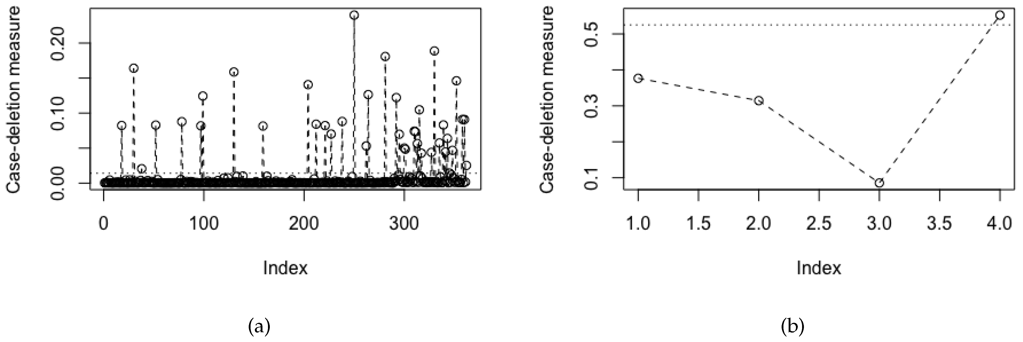
To evaluate the quality of the mixed-effects logistic regression model used in the study with asthma data, we carry out Phases II and III for data-influence analytics described in Algorithm 6. The results are the following. Figure 1 shows the index plots of global influence measures for (a) the cases with benchmark equal to 0.0141 and (b) the case-groups with benchmark equal to 0.5250. All potentially influential cases from the four groups identified from Figure 1a have been displayed in

Table 2. The indicated globally influential cases from all four groups from Figure 1 with asthma data.

Group	Case(s)
1	#18	#30	#38	#52
2	#78	#97	#99	#130	#159
3	#204	#212	#221	#227	#238
4	#292	#295	#300	#301	#310	#311	#313	#315	#317	#327	#330
	#335	#339	#341	#343	#345	#348	#352	#358	#360	#362

. In addition, Figure 1b indicates the Group 4 (severe persistent asthma) as potentially influential.

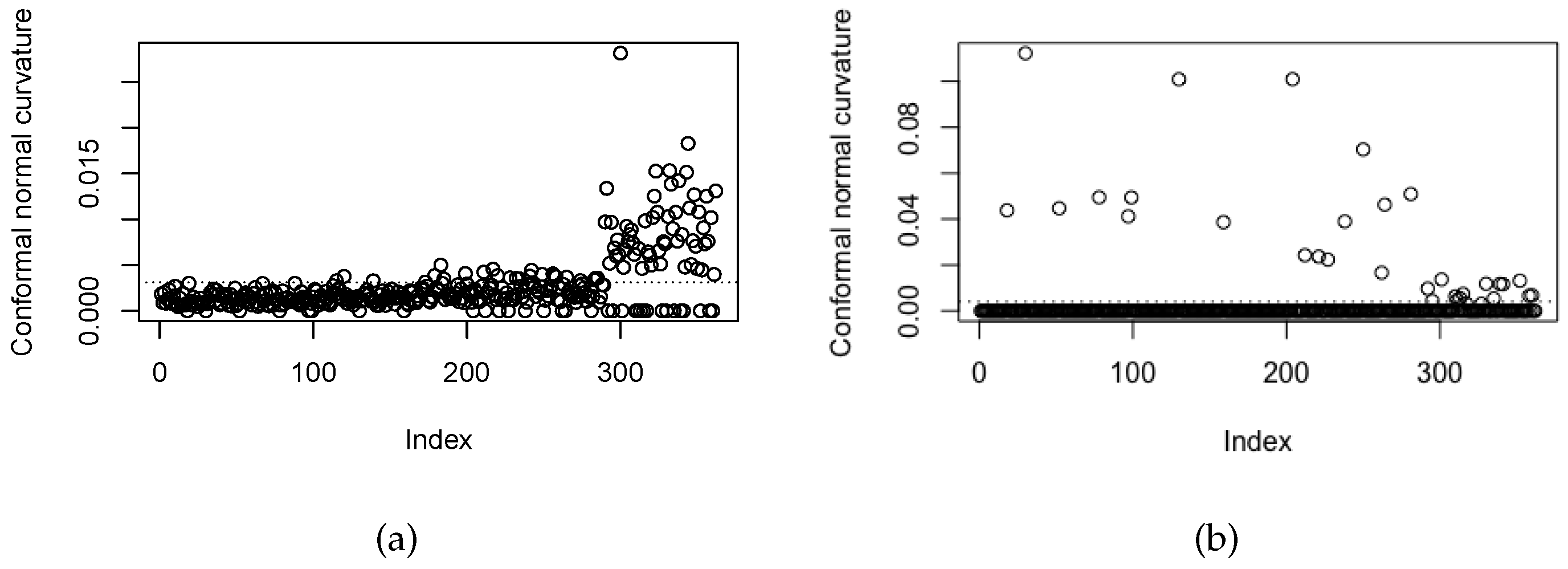
Figure 2a,b show index plots of local influence measures for (a) $y_{ij}=0$ with benchmark equal to 0.0031 and (b) $y_{ij}=1$ with benchmark equal to 0.0040. All local influence cases from four groups identified from Figure 2 are reported in

Table 3. The indicated locally influential cases from all four groups from Figure 2 with asthma data.

Group	Case(s)
1	$y_{ij}=1$	#18	#30	#52
2	$y_{ij}=0$	#115	#120	#139
2	$y_{ij}=1$	#78	#97	#99	#130	#159
3	$y_{ij}=0$	#173	#179	#183	#185	#199	#211	#217	#220
		#228	#232	#234	#241	#242	#249	#256	#257
		#258	#265	#274	#283	#284	#285
3	$y_{ij}=1$	#204	#212	#221	#227	#238	#250	#262	#264	#281
4	$y_{ij}=0$	#290	#291	#293	#294	#296	#297	#298	#299
		#300	#302	#303	#304	#305	#306	#307	#308
		#309	#312	#314	#316	#318	#319	#320	#321
		#322	#323	#324	#325	#326	#328	#329	#331
		#332	#333	#334	#336	#337	#338	#340	#342
		#343	#344	#345	#346	#347	#348	#349	#350
		#351	#353	#354	#355	#356	#357	#359	#361	#362
4	$y_{ij}=1$	#292	#295	#301	#310	#311	#313	#315	#330
		#335	#339	#341	#352	#358	#360

.

Table 4. Estimates (SE), p-values and RC under global influence diagnostics for the asthma data.

Removed Cases/Case-Groups	Effect	Parameter	Estimate (SE)	p-Value	RC
None	Intercept	${\beta }_0$	−4.0430 (0.7343)	<0.0001	-
	Treatment	${\beta }_1$	0.1871 (0.0579)	0.0012	-
	Eosinophilia	${\beta }_2$	0.1101 (0.0481)	0.0220	-
	Allergy	${\beta }_3$	−0.7006 (0.4026)	0.0817	-
	Group asthma severity	$\sigma$	0.5417	-	-
Cases
Group 4	Intercept	${\beta }_0$	−4.7891 (0.9228)	<0.0001	18.4548
	Treatment	${\beta }_1$	0.2190 (0.0787)	0.0054	17.0093
	Eosinophilia	${\beta }_2$	0.1012 (0.0615)	0.1000	8.0440
	Allergy	${\beta }_3$	−0.5844 (0.5408)	0.2798	16.5857
	Group asthma severity	$\sigma$	0.1055	-	80.5179
Group 3	Intercept	${\beta }_0$	−4.7585 (1.1449)	<0.0001	17.6993
	Treatment	${\beta }_1$	0.2017 (0.0704)	0.0041	7.8030
	Eosinophilia	${\beta }_2$	0.0946 (0.0594)	0.1114	14.0289
	Allergy	${\beta }_3$	−0.7692 (0.4823)	0.1107	9.7869
	Group asthma severity	$\sigma$	1.3676	-	152.4889
Group 2	Intercept	${\beta }_0$	−4.4838 (1.0104)	<0.0001	10.9038
	Treatment	${\beta }_1$	0.1612 (0.0629)	0.0104	13.8549
	Eosinophilia	${\beta }_2$	0.1066 (0.0539)	0.0480	3.1408
	Allergy	${\beta }_3$	−0.5427 (0.4493)	0.2271	22.5364
	Group asthma severity	$\sigma$	1.2190	-	125.0695
Group 1	Intercept	${\beta }_0$	−4.2253 (0.9174)	<0.0001	4.5107
	Treatment	${\beta }_1$	0.1814 (0.0626)	0.0037	3.0550
	Eosinophilia	${\beta }_2$	0.1116 (0.0521)	0.0323	1.4334
	Allergy	${\beta }_3$	−0.9529 (0.4247)	0.0248	35.9984
	Group asthma severity	$\sigma$	1.0386	-	91.7622
Case-groups
Group 4	Intercept	${\beta }_0$	−4.6387 (0.8633)	<0.0001	14.7364
	Treatment	${\beta }_1$	0.2097 (0.0772)	0.0066	12.0460
	Eosinophilia	${\beta }_2$	0.1075 (0.0598)	0.0723	2.2988
	Allergy	${\beta }_3$	−0.4947 (0.5453)	0.3642	29.3869
	Group asthma severity	$\sigma$	0.0000	-	-

and

Table 5. Sens, Spec and Acc measures under global influence diagnostics for the asthma data.

Removed Cases	Sens	Spec	Acc
None	0.6969	0.7598	0.7541
Cases
Group 4	0.6470	0.5740	0.5777
Group 3	0.8333	0.8328	0.8328
Group 2	0.7500	0.7598	0.7591
Group 1	0.7666	0.7713	0.7709
Case-groups
Group 4	0.6470	0.6029	0.6055

display the results of estimates, SE, p-values, RC and predictive performance measures from post-deletion analysis of the cases and case-groups detected as influential under global influence diagnostics (Phase II). Regarding to the parameter estimates of the fixed effects ($\widehat{\mathbf{\beta }}$), note that after removing the cases detected as potentially influential for each group, the estimates present moderate changes, but the estimate related to the intercept random ($\widehat{\sigma }$) presents a high change, in accordance with the RC values. In addition, inferential changes observed for the eosinophilia covariate pass from significant to not significant at 5%, when cases from Groups 3 and 4 are removed. With respect to the Sens, Spec and Acc measures, with Sens = Spec determining an optimal threshold equal to 0.1, once the potential influential cases of Groups 1, 2 and 3 are removed, the values of Sens, Spec and Acc increase considerably. Observe that the maximum values of Sens, Spec and Acc are obtained by removing the cases detected as potentially influential of Group 3, that is, 0.8333, 0.8328 and 0.8328, respectively. Under global influence analysis for the case-groups, the estimates related to fixed effects ($\mathbf{\beta }$) present moderate changes and inferential changes at 5% in the covariate eosinophilia for the Group 4. Estimate of the variance parameter associated with the distribution of the random intercept ($\sigma$) is almost zero, that is, the model does not capture the change or heterogeneity between asthma severity groups, suggesting a standard logistic regression model. In addition, after the Group 4 is removed, the values of Sens, Spec and Acc decrease.

The results of post-deletion analysis of the cases detected as influential by group under local influence diagnostics (Phase III) are presented in

Table 6. Estimates (SE), p-values and RC under local influence diagnostics for the asthma data.

Removed Cases	Effect	Parameter	Estimate (SE)	p-Value	RC
None	Intercept	${\beta }_0$	−4.0430 (0.7343)	<0.0001	-
	Treatment	${\beta }_1$	0.1871 (0.0579)	0.0012	-
	Eosinophilia	${\beta }_2$	0.1101 (0.0481)	0.0220	-
	Allergy	${\beta }_3$	−0.7006 (0.4026)	0.0817	-
	Group asthma severity	$\sigma$	0.5417	-	-
Group 4	Intercept	${\beta }_0$	−4.6895 (0.8425)	<0.0001	15.9908
	Treatment	${\beta }_1$	0.2131 (0.0740)	0.0039	13.8918
	Eosinophilia	${\beta }_2$	0.1111 (0.0574)	0.0532	0.9085
	Allergy	${\beta }_3$	−0.3300 (0.5315)	0.5345	52.8898
	Group asthma severity	$\sigma$	0.0000	-	-
Group 3	Intercept	${\beta }_0$	−4.6938 (1.1351)	<0.0001	16.0978
	Treatment	${\beta }_1$	0.2001 (0.0706)	0.0045	6.9104
	Eosinophilia	${\beta }_2$	0.0936 (0.0596)	0.1166	14.9767
	Allergy	${\beta }_3$	−0.7722 (0.4819)	0.1090	10.2169
	Group asthma severity	$\sigma$	1.3107	-	141.9941
Group 2	Intercept	${\beta }_0$	−4.4710 (0.9954)	<0.0001	10.5871
	Treatment	${\beta }_1$	0.1605 (0.0629)	0.0107	14.2306
	Eosinophilia	${\beta }_2$	0.1092 (0.0546)	0.0458	0.8277
	Allergy	${\beta }_3$	−0.5466 (0.4495)	0.0239	21.9839
	Group asthma severity	$\sigma$	1.1812	-	118.0761
Group 1	Intercept	${\beta }_0$	−4.2345 (0.9413)	<0.0001	4.7372
	Treatment	${\beta }_1$	0.1794 (0.0625)	0.0041	4.1182
	Eosinophilia	${\beta }_2$	0.1090 (0.0519)	0.0356	0.9258
	Allergy	${\beta }_3$	−0.941 (0.4246)	0.0266	34.3375
	Group asthma severity	$\sigma$	1.0965	-	102.4380

and

Table 7. Sens, Spec and Acc measures under local influence diagnostics for the asthma data.

Removed Cases/Case-Groups	Sens	Spec	Acc
None	0.6969	0.7598	0.7541
Group 4	0.6842	0.6433	0.6460
Group 3	0.8333	0.8371	0.8368
Group 2	0.7500	0.7576	0.7570
Group 1	0.7666	0.7659	0.7660

. We note that, after removing the cases detected as potentially influentials for each group, the estimates related to fixed effects ($\mathbf{\beta }$) present moderate changes in all groups and inferential changes at 5% in the covariate eosinophilia for the Groups 4 and 3. Estimate of the variance parameter associated with the distribution of the random intercept ($\sigma$) is almost zero, that is, the model not capture the change or heterogeneity between asthma severity groups, suggesting a standard logistic regression model. In relation to the Sens, Spec and Acc measures, with the selection criteria Sens = Spec determining an optimal threshold equal to 0.1, the values of Sens, Spec and Acc are equal to 0.6969, 0.7598, 0.7541, respectively, for all data. Now, after removing the cases detected as potentially influential of the Groups 1, 2 and 3, the values increase considerably. The maximum values are obtained by removing the cases detected as influential in the Group 3, that is, these values are 0.8333, 0.8371 and 0.8368, respectively. However, for the Group 4, these values decrease mainly for Spec and Acc.

According to results obtained in Phase II and III, we observe that the Groups 3 and 4 need more study (Phase IV). For that reason, we now perform post-deletion analysis considering each type of response.

Table 8. Estimates (SE), p-values and RC under the indicated influence for the asthma data.

Removes Cases	Effect	Parameter	Estimate (SE)	p-Value	RC
None	Intercept	${\beta }_0$	−4.0430 (0.7343)	<0.0001	-
	Treatment	${\beta }_1$	0.1871 (0.0579)	0.0012	-
	Eosinophilia	${\beta }_2$	0.1101 (0.0481)	0.0220	-
	Allergy	${\beta }_3$	−0.7006 (0.4026)	0.0817	-
	Group asthma severity	$\sigma$	0.5417	-	-
Global influence diagnostics
Group 4 – $y_{ij}=0$	Intercept	${\beta }_0$	−4.2754 (0.7884)	<0.0001	5.7498
	Treatment	${\beta }_1$	0.2271 (0.0627)	0.0002	21.3234
	Eosinophilia	${\beta }_2$	0.1177 (0.0494)	0.0172	6.9236
	Allergy	${\beta }_3$	−0.8470 (0.4135)	0.0405	20.8850
	Group asthma severity	$\sigma$	0.6824	-	25.9923
Group 4 – $y_{ij}=1$	Intercept	${\beta }_0$	−4.8351 (0.9692)	<0.0001	19.5934
	Treatment	${\beta }_1$	0.2044 (0.0774)	0.0083	9.2397
	Eosinophilia	${\beta }_2$	0.0954 (0.0612)	0.1189	13.2966
	Allergy	${\beta }_3$	−0.5104 (0.5396)	0.3442	27.1547
Group 3 – $y_{ij}=1$	Intercept	${\beta }_0$	−4.7585 (1.1449)	<0.0001	17.6993
	Treatment	${\beta }_1$	0.2017 (0.0704)	0.0041	7.8030
	Eosinophilia	${\beta }_2$	0.0946 (0.0594)	0.1114	14.0289
	Allergy	${\beta }_3$	−0.7692 (0.4823)	0.1107	9.7869
	Group asthma severity	$\sigma$	1.3676	-	152.4889
Local influence diagnostics
Group 4 – $y_{ij}=0$	Intercept	${\beta }_0$	−3.114 (1.8348)	0.0896	22.9617
	Treatment	${\beta }_1$	0.2228 (0.0784)	0.0044	19.0419
	Eosinophilia	${\beta }_2$	0.1034 (0.0596)	0.0824	6.0194
	Allergy	${\beta }_3$	−0.5354 (0.5362)	0.3180	23.5843
	Group asthma severity	$\sigma$	3.0947	-	471.3594
Group 4 – $y_{ij}=1$	Intercept	${\beta }_0$	−4.6965 (0.8496)	<0.0001	16.1644
	Treatment	${\beta }_1$	0.1978 (0.0710)	0.0053	5.6892
	Eosinophilia	${\beta }_2$	0.0976 (0.0582)	0.0935	11.3076
	Allergy	${\beta }_3$	−0.3334 (0.5223)	0.5232	52.4144
	Group asthma severity	$\sigma$	0.0000	-	100
Group 3 – $y_{ij}=0$	Intercept	${\beta }_0$	−3.8635 (0.7518)	<0.0001	4.4387
	Treatment	${\beta }_1$	0.1767 (0.0593)	0.0028	5.5859
	Eosinophilia	${\beta }_2$	0.1037 (0.0494)	0.0358	5.7761
	Allergy	${\beta }_3$	−0.7219 (0.4030)	0.0732	3.0360
	Group asthma severity	$\sigma$	0.5386	-	0.5519
Group 3 – $y_{ij}=1$	Intercept	${\beta }_0$	−4.6938 (1.1351)	<0.0001	16.0978
	Treatment	${\beta }_1$	0.2001 (0.0706)	0.0045	6.9104
	Eosinophilia	${\beta }_2$	0.0936 (0.0596)	0.1166	14.9767
	Allergy	${\beta }_3$	−0.7722 (0.4819)	0.1090	10.2169
	Group asthma severity	$\sigma$	1.3107	-	141.9941

and

Table 9. Sens, Spec and Acc measures with Sens = Spec under the indicated influence for asthma data.

Removed Cases		Sens	Spec	Acc
None		0.6969	0.7598	0.7541
Global influence diagnostics
Group 4 – $y_{ij}=0$		0.7575	0.7314	0.7338
Group 4 – $y_{ij}=1$		0.5882	0.5744	0.5751
Group 3 – $y_{ij}=1$		0.8333	0.8328	0.8328
Local influence diagnostics
Group 4 – $y_{ij}=0$		0.7878	0.7904	0.7901
Group 4 – $y_{ij}=1$		0.6842	0.6200	0.6235
Group 3 – $y_{ij}=0$		0.7272	0.7133	0.7147
Group 3 – $y_{ij}=1$		0.8333	0.8328	0.8328

displays the results of estimates, SE, p-values, RC and predictive performance measures, with $y_{ij}=0$ and $y_{ij}=1$ of the Groups 3 and 4. For the global influence diagnostics, the cases with responses $y_{ij}=0$ for the Group 4 lead to a significant allergy covariate at 5%. For the cases with responses $y_{ij}=1$, in both groups we conclude that the eosinophilia covariate is not significant at 5%. By observing the performance measures, after removing the cases with $y_{ij}=0$ of the Group 4, the values of these measures increase partially, whereas after removing the cases with $y_{ij}=1$ of the Group 3, the values of these measures increase substantially. For the local influence diagnostics, we observe that the cases with responses $y_{ij}=0$ and $y_{ij}=1$ of the Group 4, and cases with responses $y_{ij}=1$ of the Group 3 are related to the eosinophilia covariate which is not significant at 5%. In addition, the cases with responses $y_{ij}=1$ of the Group 4 are related to the estimate of the variance ($\sigma$), which is almost zero and this is associated with the normal distribution of the random intercept. By observing the performance measures, after removing the cases with $y_{ij}=0$ of the Group 4 and $y_{ij}=1$ of the Group 3, the values of these measures increase. Thus, we decide to remove the cases with $y_{ij}=0$ of the Group 4 and cases with $y_{ij}=1$ of the Group 3 (Phase V). This makes sense because they are patients with severe persistent asthma (Group 4) but without FAO, or they have moderate persistent asthma (Group 3) and present FAO.

Table 10. Estimates (SE), p-values and RC under data-influence analytics for the asthma data.

Removed Cases	Effect	Parameter	Estimate (SE)	p-Value	RC
None	Intercept	${\beta }_0$	−4.0430 (0.7343)	<0.0001	-
	Treatment	${\beta }_1$	0.1871 (0.0579)	0.0012	-
	Eosinophilia	${\beta }_2$	0.1101 (0.0481)	0.0220	-
	Allergy	${\beta }_3$	−0.7006 (0.4026)	0.0817	-
	Group asthma severity	$\sigma$	0.5417	-	-
Group 4 – $y_{ij}=0$	Intercept	${\beta }_0$	−4.7920 (3.2765)	0.1435	18.5261
Group 3 – $y_{ij}=1$	Treatment	${\beta }_1$	0.2987 (0.1181)	0.0114	59.6048
	Eosinophilia	${\beta }_2$	0.0916 (0.0863)	0.2883	16.7512
	Allergy	${\beta }_3$	−0.4026 (0.7687)	0.6004	42.5413
	Group asthma severity	$\sigma$	5.5658	-	927.5726

and

Table 11. Sens, Spec and Acc measures under data-influence analytics for the asthma data.

Removed Cases		Sens	Spec	Acc
None		0.6969	0.7598	0.7541
Group 4 – $y_{ij}=0$/Group 3 – $y_{ij}=1$		0.8750	0.8860	0.8851

report the results of the post-deletion analysis. Observe that the eosinophilia covariate is not significant at 5%, and allergy is not significant at 10%. Nevertheless, the Sens, Spec and Acc measures present a large increase, that is, 0.8750, 0.8860 and 0.8851, respectively.

Table 12. Estimates (SE), p-values and RC under data-influence analytics for the asthma data.

Removed Cases	Effect	Parameter	Estimate (SE)	p-Value	RC
None	Intercept	${\beta }_0$	−4.0430 (0.7343)	<0.0001	-
	Treatment	${\beta }_1$	0.1871 (0.0579)	0.0012	-
	Eosinophilia	${\beta }_2$	0.1101 (0.0481)	0.0220	-
	Allergy	${\beta }_3$	−0.7006 (0.4026)	0.0817	-
	Group asthma severity	$\sigma$	0.5417	-	-
Group 4 – $y_{ij}=0$	Intercept	${\beta }_0$	−4.7920 (3.2765)	0.1435	18.5261
Group 3 – $y_{ij}=1$	Treatment	${\beta }_1$	0.2987 (0.1181)	0.0114	59.6048
	Eosinophilia	${\beta }_2$	0.0916 (0.0863)	0.2883	16.7512
	Allergy	${\beta }_3$	−0.4026 (0.7687)	0.6004	42.5413
	Group asthma severity	$\sigma$	5.5658	-	927.5726
Group 4 – $y_{ij}=0$	Intercept	${\beta }_0$	−4.2963 (3.2379)	0.1845	6.2670
Group 3 – $y_{ij}=1$	Treatment	${\beta }_1$	0.2869 (0.1159)	0.0133	53.3056
	Group asthma severity	$\sigma$	5.7493	-	5121.0510

reports the fit for the model reduced (without these covariates), and

Table 13. Sens, Spec and Acc measures under data-influence analytics for the asthma data.

Removed Cases		Sens	Spec	Acc
None		0.6969	0.7598	0.7541
Full model
Group 4 – $y_{ij}=0$/Group 3 – $y_{ij}=1$		0.8750	0.8860	0.8851
Reduced model
Group 4 – $y_{ij}=0$/ Group 3 – $y_{ij}=1$		0.8333	0.8382	0.8378

reports the performance measures of the prediction. Note that the variance increases and that the prediction measures decrease. Hence, these covariates must remain in the model. Therefore, the method of combining the global and local influence diagnostics at the group and cases levels allow us to obtain a model with higher prediction capacity and some inferential changes.

9. Conclusions, Discussion, and Future Research

When patients belong to a specific group, such as patients classified according to their severity of asthma, the data present dependence and have a hierarchical structure that can be modeled through the use of mixed models [17]. If the interest is to analyze or predict the binary response variables of individuals based on certain variables fixed or random measured from those individuals, a mixed-effect logistic regression model can be used [17,18]. This model is a typical predictive model widely used in practice.

This research reported the following findings:

(i)

We have provided a data-influence analytics using a mixed-effect logistic regression applied to the asthma disease based on global and local influence diagnostic techniques, which are used simultaneously in this study but often used separately. Such a joint usage allowed us to identify situations which could not be identified if we use these techniques separately. In the case of our application, this data-influence analytics is provided in Table 2, Table 3, Table 4, Table 5, Table 6, Table 7, Table 8, Table 9, Table 10, Table 11, Table 12 and Table 13 and Figure 1 and Figure 2.

(ii)

We have considered predictive performance measures for these analytics. In the case of our application, results for these predictive performance measures are provided in Table 1, Table 5, Table 7, Table 9, Table 11, and Table 13.

(iii)

We have given an algorithm that summarizes the methodology proposed in this study; see Algorithm 4.

(iv)

We have proposed and implemented a methodology for the data-influence analytics of this type of predictive models, which allows the provision of improved scientific evidence in asthma data, to evaluate if the data contain particular observations that may impact on the conclusions to be drawn from the analysis and, therefore, impact the medical decision-making.

(v)

We have illustrated the proposed methodology with a case study of real-world data regarding to the asthma data collected from a public hospital at São Paulo, Brazil.

The case study has shown that the new methodology allowed us to obtain a model with the high predictive capacity, identify patients who are too different medically in relation to fixed airway obstruction values, especially for severe persistent asthma and moderate persistent asthma groups. In addition, we explained what characteristics or explanatory variables are associated with fixed airway obstruction, in order to model the probability of fixed airway obstruction given the asthma severity group in which it was classified. The results of this work can be taken as a contribution to the data-influence analytics in predictive models applied to the asthma disease. Note that improving the data quality with analytics has gained attention in recent years, especially in medicine. It allows us to identify anomalies increasing the efficiency of medical experiments, while maintaining a high level of data quality. Thus, it is possible to avoid inaccurate conclusions from results of the study. Therefore, good statistical practices must be followed with sophisticated techniques, such as those presented in this work related to detection of influential data and outliers, as well as other possible inconsistencies in the data; see the studies presented in [48,49], which support our discussion in terms of data quality and analytics in medicine. Thus, our study can be a knowledge addition to the toolkit of diverse practitioners, including medical doctors, applied statisticians, and data scientists.

Some themes for future research, which arose from the present investigation, are the following:

(i)

The procedure of data-influence analytics is very useful for identifying a set of the particular observations termed influential. However, this set may include other type of particular observations that are those so-called outliers. These outliers are those that are not well fitted by the model and their detection is based commonly on the residual analysis. Therefore, developing a methodology, which allows the identification of outliers detected in a data set using different types of residuals for mixed-effects logistic regression models, is of interest for future study about quality of fitted and prediction capability of the model [50].

(ii)

An important aspect to be considered when medical data are analyzed is censorship. Model parameter estimates with censored data is more efficient than when censorship is not considered. Indeed, if censored cases are present and a censoring is not considered, it is not possible to estimate the variance of the censored part. Nevertheless, if the censored case is used, such a variance may be estimated from the data. In addition, asymptotic behavior and performance of maximum likelihood estimators in more complex statistical models can be studied in [51,52]. Estimation methods for the regression parameters upon a high censoring may be studied by a mixture structure [53,54,55].

(iii)

An extension of the present study to the multivariate case is also of practical relevance [52,56,57].

(iv)

Incorporation of temporal, spatial, functional, and quantile regression structures in the modeling, as well as errors-in-variables, and PLS regression, are also of interest [26,29,30,58,59,60,61,62,63].

Therefore, the proposed methodology in this investigation promotes new challenges and offers an open door to explore other theoretical and numerical issues. Research on these and other issues are in progress and their findings will be reported in future articles.