Abstract
In this study, two new integrated control charts, named -MAE chart and MS-MAE chart, are introduced for monitoring the quality of a process when the mathematical form of nonlinear profile model for quality measure is complicated and unable to be specified. The -MAE chart is composed of two memoryless-type control charts and the MS-MAE chart is composed of one memory-type and one memoryless-type control charts. The normality assumption of error terms in the nonlinear profile model for both proposed control charts are extended to a generalized model. An intensive simulation study is conducted to evaluate the performance of the -MAE and MS-MAE charts. Simulation results show that the MS-MAE chart outperforms the -MAE chart with less false alarms during the Phase I monitoring. Moreover, the MS-MAE chart is sensitive to different shifts on the model parameters and profile shape during the Phase II monitoring. An example about the vertical density profile is used for illustration.
1. Introduction
Statistical process control (SPC) is the methodology for quality control using statistical methods for monitoring the quality of a process. Because it can maintain the process to be operated efficiently, produce more confirming products and reduce rework or scrap, SPC has been widely used to monitor the quality of production processes to decline the variability among products and keep their quality close to the desired level. It should also mention that the major tool, control charts, can be treated as a visualization of statistical hypothesis testing. Engineers can use control charts to process data and identify common-cause or assignable-cause variations during the production and distinguish between the process in control and the problematic variation. If the variability is due to an assignable-cause, an out-of-control signal will be flagged before large amount of nonconforming products produced. Therefore, engineers can efficiently maintain the process stable through using SPC. Comprehensive demonstrations about the fundamental to establish control charts and the applications of using control charts can be found in Montgomery [1]. In many instances, the quality of a product can be expressed as a functional form of explanatory variables. The SPC for monitoring functional form data is also named profile monitoring. Recent advances in manufacturing have been proposed, the functional form under monitoring could be complicated and contains a lot of unknown parameters. Multivariate control chart methods are efficient to simultaneously monitor the shift on the model parameters. Two concerns have been raised for using a multivariate control chart to monitor a process. Multivariate control chart methods are usually less sensitive to catch process shifts in Phase II monitoring if the data dimension is 10 or larger. Moreover, parametric multivariate control charts, for example, the Hotelling chart and multivariate exponentially weighted moving average (MEWMA) chart, are sensitive to the violation of normality assumption. If the random vectors of dependent variables do not follow a multivariate normal distribution, the false alarm rate (FAR) is usually inflated and over the nominal level. The FAR in the Phase I monitoring of quality control is also known as the type I error in statistical hypothesis testing methods. The EWMA-type control chart is more sensitive to a small to moderate shift on the process parameter due to using memory-type statistics to establish the control chart.
In profile monitoring, the parameters of interest are often the relationship between the response and explanatory variables and the nature of the variance between and within the profiles. Multivariate control charts are often unable to well monitor the relationship between the response and explanatory variables and the autocorrelation between the observations. In many occasions, more than ten sampling points per profile are measured as data and this fact makes the design for a multivariate control chart method cumbersome. Most of the existing profile monitoring methods assume that the error terms follow a normal distribution to develop the monitoring scheme. How to expand the normality assumption of error terms to a generalized model is also an important issue for profile monitoring.
B-spline approximation is a nonparametric method, which has been used to characterize the functional relation between the response variable and explanatory variables without subjective setting a nonlinear functional form. In the the area of numerical analysis, a B-spline or basis spline is a spline function, which has a minimal support with respect to a given degree, smoothness, and domain partition. Any fixed-degree spline function can be expressed as a linear combination of the B-spline with that degree. The B-spline curve can be used for curve-fitting for a nonlinear data set. The advantage of using a B-spline curve is given as follows: B-spline curve is a generalization of the Bézier curve. The B-spline uses polynomial curve for establishment and requires the information regarding the degree of the curve, a knot vector and a more complex theory than Bézier curves. A B-spline curve can be a Bézier curve. Moreover, the B-spline curve satisfies all important properties that the Bézier curves has. The B-spline curve has more control flexibility than the Bézier curve for modeling. For example, the user can use a lower degree B-spline curve to maintain a large number of control points. The user can change the position of a control point without globally changing the shape of the whole curve based on the local modification property. The B-spline curve can provide a finer shape control due to it satisfies the strong convex hull property. Many techniques for designing and editing the shape of a curve can be done such as changing the knots in a B-spline curve.
Chang and Yadama [2] used the B-spline approximation method to characterize the shape of nonlinear profile and split the nonlinear profile into several sets to reduce the dimension of input variables. After using dimension reduction techniques and doing data transformation, Chang and Yadama [2] suggested using traditional control chart methods for monitoring nonlinear profile processes. Chuang et al. [3] combined the B-spline approximation and control chart methods to develop a nonparametric SPC method for monitoring profile data. Their monitoring method includes five steps: data cleaning, fitting B-spline models, resampling for response data using block bootstrap method, constructing the confidence band based on bootstrap curve depths, and monitoring profiles online based on curve matching. Winistorfer et al. [4] used B-spline approximation and Wavelet transformation methods to construct control charts for monitoring vertical density profile (VDP) data. The VDP is the density distribution through the panel thickness to measure the quality of a wood-based composite panel about its well with strength and physical properties. Woodall et al. [5] discussed some of the general profile monitoring issues via using control chart methods. They also gave a comprehensive review for related SPC literature about profile monitoring. Chang and Chou [6] provided a general discussion about using the Wavelet transformation and B-spline approximation methods for monitoring nonlinear profile models. Hadidoust et al. [7] proposed a Phase II B-spline approximation monitoring method to detect the change-point in a nonlinear profile process.
Fan et al. [8] suggested a Phase II nonlinear profile monitoring procedure via using the transformation of the sum of sine functions. Their method can tackle complicated nonlinear functional form of profiles through heavy numerical computation. Shiau et al. [9] aimed at constructing monitoring schemes for the nonlinear profile model of random effects. They proposed to use principal component method to obtain principal component scores and then use the principal component scores to construct Hotelling chart. Vaghefi et al. [10] proposed two approaches for monitoring nonlinear profile processes: the first approach was to use control chart method with parametric estimates from a regression model as inputs and the second approach was to use metrics to measure the deviation from a reference curve to escape the complexity problems from the coefficient estimation of nonlinear profiles. Williams et al. [11] used Hotelling chart to monitor the coefficients of a parametric nonlinear regression model for a profile process. They used three general formulation methods for the statistics and suggested statistical methods to determine the Phase I control limits. Boullosa-Falces et al. [12] studied the methods to detect small and sudden deviations in the fuel oil process of marine diesel engine when the correlations between input variables were low. They proposed a monitoring method to combine the Hotelling and cumulative sum (CUSUM) charts. The CUSUM chart is also a memory-type control chart, which is developed based on the cumulative sum statistics.
Three concerns in current existing works on nonlinear profile monitoring in literature are stated as: (1) the nonlinear profile model is complicated and difficult to be expressed as an explicit mathematical form in some instances; (2) the existing control chart methods often assume that the error terms in a nonlinear profile model are independent and follow a normal distribution; or (3) the current existing nonlinear profile control chart could not detect process shift when the process shift is due to both the model parameters and profile shape shift together. To enhance the applicability of the control chart methods, expanding the normality assumption of error terms to a generalized distribution family is imperative. Moreover, the proposed nonlinear profile control chart methods are expected more sensitive to alarm the process shift on the model parameters or profile shape during the Phase II monitoring.
B-spline approximation methods are easy for implementation and can be used to fit a lot of nonlinear profile models. In this study, the cubic B-spline curve is used to model nonlinear profile data and then two integrated control charts are proposed for process monitoring. The first integrated chart is to combine the Hotelling chart and the mean absolute error (MAE) chart and named -MAE chart. The second integrated chart is to combine the multivariate sign exponentially weighted moving average (MSEWMA) chart and the MAE chart and named MS-MAE chart. Because both Hotelling and MAE charts are memoryless-type control charts and the MSEWMA chart is a memory-type control chart. Hence, the -MAE method is composed of two memoryless-type control charts and the MS-MAE chart is composed of one memory-type and one memoryless-type control charts. The Hotelling chart is a parametric control chart and the MSEWMA and MAE charts are nonparametric control charts.
The MSEWMA chart was originally proposed by Zou and Tsung [13]. They have shown the MSEWMA chart has some appealing properties. The MSEWMA statistic is fast to compute and is affine invariant. Moreover, for the distributions with elliptical directions, the charting sequence is a Markov chain process. Then, the in-control average run length (ARL) can be evaluated. The ARL is the expected run length of the interval between out-of-control events. The ARL in Phase I monitoring is a reference measure to design control charts. Compared with the MEWMA chart, the MSEWMA chart is more robust for in-control performance and more sensitive to the small and moderate shifts in location parameters for skewed and heavy-tailed multivariate observations. Zi et al. [14] proposed a distribution-free robust procedure based on using rank-based regression method to reduce the impact from the violation of multivariate normal distribution. Their proposed method is efficient to monitor linear profile processes. In this study, we use Monte Carlo simulations to evaluate the performance of the proposed -MAE chart and MS-MAE chart, and then the best control chart method is recommended to monitor nonlinear profile data.
The rest of this manuscript is organized as follows: The construction of the -MAE chart and MS-MAE chart via using the cubic B-spline approximation method are studied in Section 2. In Section 3, Monte Carlo simulations are conducted to verify whether the -MAE chart and MS-MAE chart can be operated close to the nominal level of FAR during the Phase I monitoring. The performance of the recommended control chart method for out-of-control Phase II monitoring is also evaluated using simulations. The strengths and weaknesses of using the proposed control chart method and the deep learning method of Autoencoder to monitor the quality of a nonlinear profile process are discussed, too. Section 4 demonstrates the application of the recommended control chart method with a re-generated data set for a real example regarding the VDP quality of particleboards. Some concluding remarks are given in Section 5.
2. The B-Spline Approximation and Control Charts
2.1. B-Spline Approximation
To trace the mathematical notations used in the proposed control chart method, a list of mathematical notations is given at the end of the paper for reference. Let Y and X denote the response and explanatory variables, respectively. The realizations of data are denoted by , in the jth profile for . The response variable can be expressed as a functional form of through the following model:
where is a nonlinear function, and is an random error. The explicit mathematical function form of could be complicated and unable to be specified in practical applications. In this study, the error terms are assumed to follow a skew-normal distribution (SND), its probability density function (PDF) can be defined by
where and are the location and scale parameters, respectively, and is the skewness parameter, which controls the skewness of the SND, see Azzalini [15] and Su et al. [16]. The SPC applications via using the SND for Shewhart control chart, economic control chart and control chart for monitoring the quality of linear profile process can be found in Tsai [17], Li et al. [18], Su et al. [19], and Li and Tsai [20]. Denote the SND by SN here and after. When , SN reduces to a normal distribution. The mean and variance of can be obtained by
and
respectively. Let , it can be shown that . The error terms are independent and follow the SN.
In practice, an order-d B-spline function can be used to approximate the nonlinear function . Let denote control points, be non-decreasing knots in the range of t, and be a set of basis functions of order d, The nonlinear function can be represented by
where
and for the coefficients of Equation (7). The basis functions , have the following properties:
- (i)
- Partition of unity: .
- (ii)
- Positivity: .
- (iii)
- Local support: if .
- (iv)
- Continuity: the th derivation of is continuous.
Each knot span is mapped onto a polynomial between and . Define knots in the interval . The first and last d knots are set to be and , and the middle knots can be chosen to be equidistant. The normalization of the knots resulting in and is helpful to improve numerical accuracy in floating point arithmetic computation. Because a cubic B-spline with is sufficient to approximate most nonlinear curves in realistic applications. In this study, the cubic B-spline method is used to approximate the nonlinear function . A comprehensive review for using R codes to implement cubic B-spline approximation can be found in de Boor [21] and Perperoglou et al. [22]. Let m in-control profile data sets be collected as Phase I samples. A multivariate control chart for monitoring nonlinear profile processes can be obtained through the following two steps:
- Step 1:
- Use a cubic B-spline to approximate in Model (1) and obtain the estimates of spline coefficients and the predicted value of , for , .
- Step 2:
- The residuals can be obtained by , . Treat the residuals , from the jth profile as a random sample from and find the maximum likelihood estimates (MLEs) of and for each profile and denoted them by and , respectively, for . Let , . Then a multivariate control chart can be constructed based on the Phase I sample , .
The Hotelling chart and MSEWMA chart are used to develop the proposed monitoring methods. The Hotelling chart is a multivariate extension of the Shewhart-type chart, which is a memoryless-type control chart. The MSEWMA chart is a nonparametric version of the MEWMA chart, which is a memory-type control chart. In general, a memory-type control chart can alarm quicker for out-of-control in Phase II than a memoryless-type control chart, and a parametric control chart is easier to establish than a nonparametric control chart. However, if the normality assumption of the quality variables is violated, then the FAR of the parametric control chart could be inflated and over the nominal level.
2.2. The New Proposed Methods
Let the Phase I sample be , ,
and
The Hotelling statistics can be represented by
The control limit in Phase I is
where is the upper th quantile of the beta distribution with parameters and . The control limit in Phase II is
where is the upper th quantile of the F distribution with degrees of freedom p and . If m is large, , where is the upper th quantile of the chi-square distribution with degrees of freedom p.
It is known that a memoryless-type control chart is insensitive to a small or moderate shift on the process parameter. Among all memory-type control charts, the EWMA-type chart is easy to implement and can quickly alarm for small to moderate shifts of the process parameter. The EWMA chart for univariate process is insensitive to the violation of normality assumption; but the MEWMA chart, which is a multivariate version of the EWMA control chart, is very sensitive to the violation of multivariate normal distribution assumption. It is known that the FAR for the MEWMA chart will be inflated and over the nominal level if the random vectors do not follow a multivariate normal distribution.
Because the domain of is , the vector of does not follow a bivariate normal distribution. In this case, the MSEWMA chart proposed by Zou and Tsung [13] can be considered to implement the process monitoring. The construction of the MSEWMA control chart is addressed as follows: Let . Two unknown parameters, the and , are needed to construct MSEWMA statistics. They can be estimated based on the Phase I sample . Let
The MSEWMA series can be defined by
where is the initial value and is a constant. In general, and 0.2 are two widely used parameters for implementing the MSEWMA chart. Based on the MSEWMA series in Equation (12), the MSEWMA statistic can be defined by
The process is claimed as out-of-control if . The is a positive control limit. Zou and Tsung [13] have provided tables to report the reference values of , those reference values were obtained by simulations.
Let and be the estimates of and , respectively. The values of and can be searched based on the iterations proposed by Hettmansperger and Randles [23].
- Step 1:
- Obtain the initial value of by
- Step 2:
- For iteration , search the value of that satisfies Equation (15), given :In practical applications, the value of can be searched based on the Step(a)-Step(e), see Tyler [24]:
- Step (a):
- Let initial value of be .
- Step (b):
- Evaluate the value of by .
- Step (c):
- Choose the value of such that the condition is true by using Cholesky decomposition method for the positive definite matrix .
- Stpe (d):
- Update by
- Stpe (e):
- Repeat the Steps (b) to (d) until convergence.
- Step 3:
- Update by ,where , .
- Step 4:
- Let . Repeat Step 2 to Step 3 untilwhere e is a predetermined small positive number. The vales of and at the final iteration when the algorithm is stopped can be the and , respectively.
The MSEWMA chart and Hotelling chart are insensitive to the shift on the profile shape. Hence, we suggest to integrate the MSEWMA chart (or Hotelling chart) with the MAE chart, and name the new integrated chart by MS-MAE chart (or -MAE chart). The MAE for profile j is defined by
Let the upper control limit of the MAE chart be , which is the upper th quantile such that . In practice, we can use the empirical distribution of to obtain an approximated value of when m is large. Let the FARs of the MSEWMA (or Hotelling ) and MAE charts be and , respectively. Then, the overall FAR can be ; that is, we can select the values of and to maintain the overall FAR at the desired level. For example, if we can take to construct the proposed MS-MAE chart or -MAE chart, the overall FAR of the integrated chart is . The corresponding ARL for the in-control Phase I process is about 185. The two integrated control charts can be implemented through using the following Step 1 to Step 4:
- Step 1:
- Obtain the estimates of and the residuals based on m in-control Phase I subgroups by using the proposed estimation method in Section 2.1.
- Step 2:
- Step 3:
- The first control chart in the integrated control chart can be the Hotelling chart or MSEWMA chart. The second control chart in the integrated control chart is the MAE chart. Let the FAR in the first and second control charts are and , respectively, and the overall FAR is .
- Step 3.1:
- The control limits in Equations (9) and (10) with can be used to establish the Hotelling .
- Step 3.2:
- The control limit of the MSEWMA chart with can be selected from the tables proposed by Zou and Tsung [13] or we can search the control limit via using simulation methods.
- Step 3.3:
- The quantile, , based on the empirical distribution of can be obtained as the control limit of MAE chart.
- Step 4:
- The -MAE chart is to integrate the Hotelling and MAE charts in Step 3 and the MS-MAE chart is to integrate the MSEWMA and MAE charts in Step 3.
3. Monte Carlo Simulations and Discussions
3.1. Performance Evaluation
The R language codes with the packages of “sn”, “splines” and “optim” are used to generate random samples from the SND, implement the B-spline approximation and obtain the estimates of the model parameters, respectively. After the proposed two integrated control charts are established, a simulation study is conducted with has two goals. The Goal 1 is to study whether the proposed integrated control charts of the -MAE chart and MS-MAE chart can be maintained at the nominal FAR level for the in-control Phase I monitoring. The Goal 2 is to study the speed to alarm of the recommended integrated control chart for parameter shifts in Phase II monitoring when the process is out of control. Nonlinear profile data are simulated using Equation (20), which was proposed in Noorossana et al. [25] for the VDP data:
for and . The total 24 sets of given by Noorossana et al. [25] are used to generate nonlinear profiles, we take the median of each set of for to generate the reference nonlinear profile for simulations in this section, and the parameters used to generate the reference nonlinear profile are , , , , and . Following the suggestions of Noorossana et al. [25], Equations (1) and (2) with , and are used to generate total pairs of for profile j. Each generated data set can be used to obtain one vector of and one . All and , , are used to construct the -MAE and MS-MAE charts with the FARs . Hence, the overall FAR for two integrated control charts are . The nominal in-control Phase I ARL is about 185, denoted by ARL = 185.
Figure 1 reports the simulated values of ARL of the MS-MAE chart with = 0.2 and the -MAE chart. Figure 1 shows that the simulated ARL of the MS-MAE chart is very closed to the nominal value when the number of samples . However, the simulated ARL of the -MAE chart always seriously underestimates the nominal ARL even the number of samples increases to 2000. It is found that the Hotelling chart has more false alarms than the MAE chart. Because the input vectors of do not follow a bivariate normal distribution, the -MAE chart causes more false alarms for monitoring the parameter estimates than the expectation. Hence, the -MAE chart is not a suitable tool for monitoring nonlinear profile data in this study. We recommend using the MS-MAE chart to monitor nonlinear profile processes. Hence, only the ability of the MS-MAE chart for detecting process shifts in Phase II is studied in the following simulations.
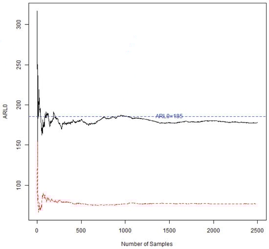
Figure 1.
The simulated values of ARL for the MS-MAE chart (solid line) and -MAE chart (dash line).
For generating out-of-control profile data to evaluate the performance of the MS-MAE chart to capture the shift of the curve at different profile locations, 10,000 data sets, 10,000, are generated based on Equation (20). Then all generated data set are fitted by Model (21) via using the package splines of the software R, where , , ⋯, are parameters and , are basis functions in the cubic B-spline approximation method.
Let and the estimate of based on the jth data set be denoted by , 10,000. In the following simulation study, we use the mean vector, , as the in-control vector of nominal parameters for the nonlinear profile model. Ten scenarios of profile shifts, labeled by Shift 1 to Shift 10 and given as follows, are considered for Phase II monitoring:
- Shift 1:
- Shift 2:
- Shift 3:
- Shift 4:
- Shift 5:
- Shift 6:
- Shift 7:
- Shift 8:
- Shift 9:
- Shift 10:
Figure 2 shows the positions of profile shape shift. Shift 1 to Shift 5 indicate that the curve shifts to its inside at different locations of the reference profile, and Shift 6 to Shift 10 indicate that the curve shifts to its outside at different locations of the reference profile. Shift 1 and Shift 6 indicate that the curve shifts at the upper-side arm of the reference profile; Shift 2 and Shift 7 indicate that the curve shifts at the middle bottom of the reference profile; Shift 3 and Shift 9 indicate that the curve shifts at the right bottom the reference profile; and Shift 4 and Shift 10 indicate that the curve shifts at the left bottom of the reference profile.
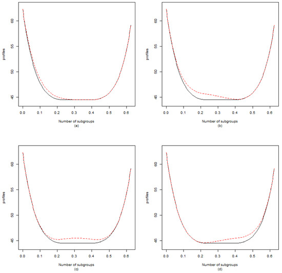
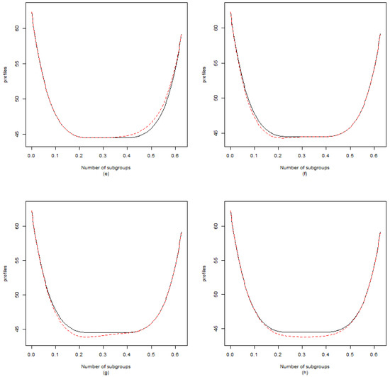
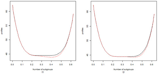
Figure 2.
The reference profile (solid line) and the out-of-control profile (dash line) (a) Shift 1 (b) Shift 2 (c) Shift 3 (d) Shift 4 (e) Shift 5 (f) Shift 6 (g) Shift 7 (h) Shift 8 (i) Shift 9 (j) Shift 10.
The control limits of the MS-MAE chart is obtained with the FARs = and the overall FAR can be maintained at . The ARL in Phase II to alarm an out-of-control case is labeled as ARL, which is evaluated based on 10,000 runs of simulation for each of the combinations of the SND parameters (1,1),(1,3), (3,1), (3,3), (5,1) and (5,3), respectively. The smaller the ARL is, the better of the ability of the control chart to alarm an out-of-control signal. Moreover, the corresponding standard deviation of run length (SDRL) for each shift, from Shift 1 to Shift 10, is respectively evaluated based on 10,000 simulation runs, too. All simulation results are reported in Table 1 for and in Table 2 for .

Table 1.
The ARL and SDRL of the MS-MAE chart for different combinations of , and .
Table 2.
The ARL and SDRL of the MS-MAE chart for different combinations of , and .
In view of Table 1 and Table 2, it can be noticed that the proposed MS-MAE chart is sensitive to alarm the shift at different locations of the reference curve with a short ARL. When the scale parameter of the SND is large or the SND is highly skewed, the ability of the MS-MAE chart to alarm out-of-control is reduced. When or in the SND become large, the MS-MAE chart needs more time or a longer ARL to alarm out of control in Phase II. Moreover, Table 1 and Table 2 also show that the MS-MAE chart with = 0.1 and MS-MAE chart with = 0.2 are competitive. Both charts have two close values of ARL to alarm process shifts for the same parameter combination of and . The SDRL in Table 1 and Table 2 are also close for the same parameter combination of and . Overall, the MS-MAE chart with can alarm out of control a little quicker than the MS-MAE chart with .
3.2. Discussions
Today, deep learning methods have earned more attention in machine learning applications. Deep learning refers to multi-layer neural networks, which can learn complex patterns for pattern recognition. If we treat the control chart method as an issue of pattern recognition, the deep leaning methods are competitive with the proposed control chart method. The Autoencoder is one popular deep learning method in an unsupervised manner. The Autoencoder can be used to learn a representation of encoding for a data set via training the network to ignore the signal of noise for dimensionality reduction. A reconstructing side is learnt from the reduction side, in which the Autoencoder tries to copy its input to its output to maintain the representation as close as possible to its input. An internal or hidden layer in an Autoencoder can be used to describe a code for representing the input, and it is composed of two main parts: an encoder and decoder for mapping the input into the code and mapping the code into a reconstruction of the input, respectively. The idea of Autoencoder has been widely applied in neural networks for deep learning in the past few decades.
As other deep learning algorithms, the Autoencoder requires large amounts of data for training via intensive computation. Moreover, the Autoencoder requires much more expertise to set the architecture and hyper-parameters. Hence, the Autoencoder could be unsuitable as a general-purpose algorithm. In many occasions of quality control, it could be difficult to offer large amounts of data for training model in a deep learning algorithm due to the considerations of sampling cost, destructive testing or other reasons. The proposed control chart method uses a cubic B-spline curve to characterize nonlinear profile data and monitor the quality of a process via using an integrated control chart. The proposed control chart method could be less effective than the Autoencoder algorithm to process a broad nonlinear functions. However, the proposed control chart method requires less sample resource to obtain reliable monitoring results than using a machine learning method. As we have mentioned in the literature review in Section 1, the cubic B-spline function has been proved to well approximate a lot of nonlinear functions in quality control applications. When the sample resource is limited for training model, the proposed control chart method is competitive for monitoring the quality of a nonlinear profile process. If large amounts of data can be offered by a nonlinear profile process for training model, the Autoencoder algorithm can be considered to replace the proposed control chart method for process monitoring. By the way, how to conduct a diagnostic process for identifying the causes of out of control via using a deep learning algorithm for process monitoring is still an open question in SPC.
4. An Application
In this section, an example regarding monitoring the quality of particle boards is used for illustration. The VDP through the panel thickness has been identified as an important panel characteristic, which is related to the strength and physical properties of particleboards. A profilometer is used to monitor the density of the finished particle boards over time at fixed depths across the thickness of the particle board during the manufacturing of particle boards. Density measurements for the VDP data were taken at depths , to give a sample of , , .
Because we do not have the original data set, the process proposed by Noorossana et al. [25] is followed to generate VDP data sets for illustration. Equation (21) with the obtained in Section 3, based on in-control Phase I samples with = 1 and = 3, is used to generate 50 in-control Phase I nonlinear profiles, and we use to generate additional 25 out-of-control profiles; that is, the SND parameters of and do not shift, but the profile shape shifts at its right side as that in Figure 2g. Using the FARs and for the in-control Phase I monitoring, the numerical control limits = 8.567 and can be obtained via using simulations for the MS-MAE chart with . The MS-MAE chart for this data set is given in Figure 3. The MSEWMA control chart in the MS-MAE method is used to monitor the parameters and , and the MAE control chart is used to monitor the shift on the profile shape.The MS-MAE chart triggers a signal for out of control at profile 52, and then several out-of-control signals follow. In scan of Figure 3, we find that the MSEWMA chart does not alarm for out of control but the MAE chart triggers out-of-control signals at profile 52 and after. Therefore, the MS-MAE chart can quickly alarm out-of-control in this example.
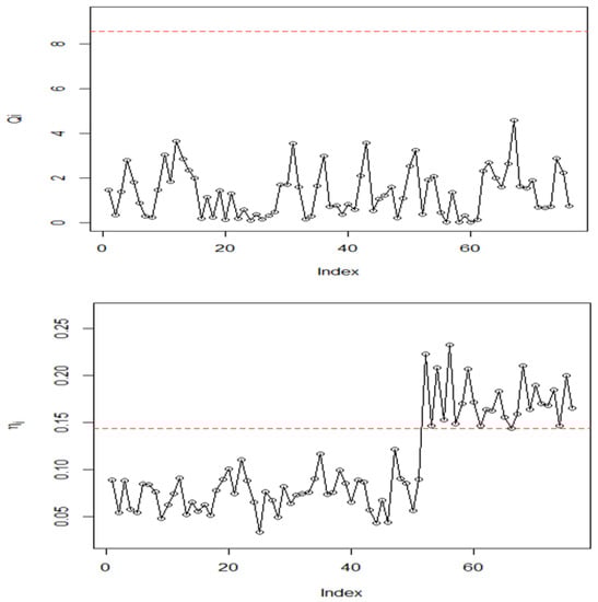
Figure 3.
The MS-MAE chart for the VDP data set.
5. Concluding Remarks
In this study, two new integrated control charts, the -MAE chart and MS-MAE chart, are proposed to monitor nonlinear profile data when the mathematical form of the nonlinear profile model is complicated and unable to be specified. Moreover, the error terms in the nonlinear profile model are assumed to follow a SND, which is a generalized version of the normal distribution. The cubic B-spline approximation method is used for modeling the profile data, and the residuals are used to obtain the MLEs of the SND parameters.
Monte Carlo simulations are conducted to verify the performance of the proposed -MAE chart and MS-MAE chart. The simulation results have shown that the -MAE chart was unable to perform well due to the input vector of the MLEs of the SND parameters does not follow a bivariate normal distribution. The FAR of the -MAE chart highly overestimates the nominal value of the FAR in the Phase I monitoring. The MS-MAE chart is more reliable than the -MAE chart. Moreover, the MS-MAE chart is sensitive to alarm the process shifts on the distribution parameters or profile shape. The re-generated VDP data sets of particle boards have been used to show that the proposed MS-MAE chart can quickly alarm out of control in Phase II monitoring. If large amounts of data can be offered by a production process for training model, the deep learning method via using the Autoencoder algorithm can be considered to replace the proposed control chart method for process monitoring.
This study focuses on providing a general control chart method to monitor the quality of a nonlinear profile process. The VDP data is used for illustration. However, the proposed method can be used to monitor any nonlinear profile process with data that can be characterized via using a cubic B-spline approximation. In view of the simulation results, the parameter estimation for the SND was found not stable if the sample size in each profile is small. How to obtain reliable parameter estimation for the SND via using other algorithms is an open question. It also is important to reduce the sample resource to establish the MSEWMA chart in the proposed control chart method. Some machine learning methods are also competitive for the process monitoring purpose. However, the sample resource limitation is a problem for many production processes. How to conduct a efficient diagnostic process for identifying the out-of-control causes via using a deep learning algorithm for process monitoring is still an open question in SPC. It is also important to design a new control chart based on the economical purposes or conditions for monitoring the quality of a process. These topics will be studied in the future.
Author Contributions
All authors equally contributed in writing this manuscript. All authors read and approved the final manuscript.
Funding
This study is supported by the grant of Northeast Petroleum University, Heilongjiang, China, NO.: 2020YDL-07.
Acknowledgments
Tzong-Ru Tsai appreciates the support from the grant of Ministry of Science and Technology, Taiwan MOST 108-2221-E-032-018-MY2.
Conflicts of Interest
The authors declare no conflict of interest.
Abbreviations
| response variables | |
| explanatory variables | |
| nonlinear function | |
| random error | |
| the number of points in profile j | |
| probability density function | |
| , , | the location, scale and skewness parameters of the SND |
| , | real number and positive real number |
| control point in B-spline function | |
| t, | non-decreasing knots |
| d | the order of basis function |
| the basis function of order d in B-spline function | |
| the end points of an interval | |
| the predicted value of | |
| residuals | |
| m | the number of subgroups in Phase I |
| the vector of | |
| The control limit of the control chart based on Hotelling statistics | |
| , | false alarm rates |
| p | the dimension of an input vector |
| the upper th quantile of the beta distribution with degrees of freedom and | |
| the upper th quantile of the F distribution with degrees of freedom p and | |
| the upper th quantile of the chi-square distribution with degrees of freedom p | |
| , | MSEWMA series |
| , | a matrix of unknown constants to construct a MSEWMA series and the estimate of |
| , , | the constants in MSEWMA series and the estimate of |
| identity matrix of order p | |
| , | matrices to obtain and |
| , | vector to obtain |
| e | a threshold of error to reach convergence |
| the upper th quantile of the sampling distribution of | |
| the coefficients of for VDP data | |
| , | coefficients in the cubic B-spline model for VDP data; |
References
- Montgomery, D.C. Statistical Quality Control: A Modern Introduction, 7th ed.; John Wiley & Suns, Ltd.: Hoboken, NJ, USA, 2013. [Google Scholar]
- Chang, S.I.; Yadama, S. Statistical process control for monitoring non-linear profiles using wavelet filtering and B-Spline approximation. Int. J. Prod. Res. 2010, 48, 1049–1068. [Google Scholar] [CrossRef]
- Chuang, S.-C.; Hung, Y.-C.; Tsai, W.-C.; Yang, S.-F. A framework for nonparametric profile monitoring. Comput. Ind. Eng. 2013, 64, 482–491. [Google Scholar] [CrossRef]
- Winistorfer, P.; Young, T.; Walker, E. Modeling and comparing vertical density profiles. Wood Fiber Sci. 1996, 28, 133–141. [Google Scholar]
- Woodall, W.H.; Spitzner, D.J.; Montgomery, D.C.; Gupta, S. Using control charts to monitor process and product quality profiles. J. Qual. Technol. 2004, 36, 309–320. [Google Scholar] [CrossRef]
- Chang, S.I.; Chou, S.H. A study of using Wavelet transformation and B-spline approximation for nonlinear profiles monitoring. In Proceedings of the 2009 Industrial Engineering Research Conference (IERC), Miami, FL, USA, 30 May–3 June 2009; pp. 1567–1572. [Google Scholar]
- Hadidoust, Z.; Samimi, Y.; Shahriari, H. Monitoring and change-point estimation for spline-modeled non-linear profiles in phase II. J. Appl. Stat. 2015, 42, 2520–2530. [Google Scholar] [CrossRef]
- Fan, S.-K.; Chang, Y.-J.; Aidara, N. Nonlinear profile monitoring of reflow process data based on the sum of sine functions. Qual. Reliab. Eng. Int. 2013, 29, 743–758. [Google Scholar] [CrossRef]
- Shiau, J.-J.H.; Huang, H.-L.; Lin, S.-H.; Tsai, M.-Y. Monitoring nonlinear profiles with random effects by nonparametric regression. Commun. Stat. Theory Methods 2009, 38, 1664–1679. [Google Scholar] [CrossRef]
- Vaghefi, A.; Tajbakhsh, S.D.; Noorossana, R. Phase II monitoring of nonlinear profiles. Commun. Stat. Theory Methods 2009, 38, 1834–1851. [Google Scholar] [CrossRef]
- Williams, J.D.; Woodall, W.H.; Birch, J.B. Statistical monitoring of nonlinear product and process quality profiles. Qual. Reliab. Eng. Int. 2007, 23, 925–941. [Google Scholar] [CrossRef]
- Boullosa-Falces, D.; Barrena, J.L.L.; Lopez-Arraiza, A.; Menendez, J.; Solaetxe, M.A.G. Monitoring of fuel oil process of marine diesel engine. Appl. Therm. Eng. 2017, 127, 517–526. [Google Scholar] [CrossRef]
- Zou, C.; Tsung, F. A multivariate sign EWMA control chart. Technometrics 2011, 53, 84–97. [Google Scholar] [CrossRef]
- Zi, X.; Zou, C.; Tsung, F. A distribution-free robust method for monitoring linear profiles using rank-based regression. IIE Trans. 2012, 44, 949–963. [Google Scholar] [CrossRef]
- Azzalini, A. A class of distributions which includes the normal ones. Scand. J. Stat. 1985, 12, 171–178. [Google Scholar]
- Su, N.-C.; Gupta, A.K. On some sampling distributions for skew-normal population. J. Stat. Comput. Simul. 2015, 85, 3549–3559. [Google Scholar] [CrossRef]
- Tsai, T.-R. Skew Normal Distribution and the design of control charts for averages. Int. J. Reliab. Qual. Saf. Eng. 2007, 14, 49–63. [Google Scholar] [CrossRef]
- Li, C.-I.; Su, N.-C.; Su, P.-F.; Shyr, Y. The design of X¯ and R control charts for skew normal distributed data. Commun. Stat. Theory Methods 2014, 43, 4908–4924. [Google Scholar] [CrossRef]
- Su, N.-C.; Chiang, J.-Y.; Chen, S.-C.; Tsai, T.-R.; Shyr, Y. Economic design of two-stage control charts with skewed and dependent measurements. Int. J. Adv. Manuf. Technol. 2014, 73, 1387–1397. [Google Scholar] [CrossRef]
- Li, C.-I.; Tsai, T.-R. Linear profiles monitoring in the presence of nonnormal random errors. Qual. Eng. Int. 2019, 35, 2579–2592. [Google Scholar] [CrossRef]
- de Boor, C. A Practical Guide to Spline, rev. ed.; springer: Berlin, Germany, 2003; ISBN 0-387-95366-3. [Google Scholar]
- Perperoglou, A.; Sauerbrei, W.; Abrahamowicz, M.; Schmid, M. A review of spline function procedures in R. BMC Med. Res. Methodol. 2019, 19, 19–46. [Google Scholar] [CrossRef]
- Hettmansperger, T.P.; Randies, R.H. A practical affine equivariant multivariate median. Biometrika 2002, 89, 851–860. [Google Scholar] [CrossRef]
- Tyler, D.E. A distribution-free M-estimator of multivariate scatter. Ann. Stat. 1987, 15, 234–251. [Google Scholar] [CrossRef]
- Noorossana, R.; Saghaei, A.; Amiri, A. Statistical Analysis of Profile Monitoring; Wiley: Hoboken, NY, USA, 2011; ISBN 9780470903223. [Google Scholar]
© 2020 by the authors. Licensee MDPI, Basel, Switzerland. This article is an open access article distributed under the terms and conditions of the Creative Commons Attribution (CC BY) license (http://creativecommons.org/licenses/by/4.0/).