Abstract
This paper puts forward a PD-type iterative learning control algorithm for a class of discrete spatially interconnected systems with unstructured uncertainty. By lifting and changing the variable of discrete space model, the uncertain spatially interconnected systems is converted into equivalent singular system, and the general state space model is derived in view of singular system theory. Then, the state error and output error information are used to design the iterative learning control law, transforming the controlled system into an equivalent repetitive process model. Based on the stability theory of repetitive process, sufficient condition for the stability of the system along the trial is given in the form of linear matrix inequalities (LMIs). Finally, the effectiveness of the proposed algorithm is verified by the simulation of ladder circuits.
1. Introduction
Iterative learning control (ILC) is applicable to the controlled systems that repeatedly perform the same finite-time operation task, with the goal to achieve accurate tracking of the reference trajectory. Each execution is known as a trial (or pass) and the finite duration the trial (or pass) length. The most fascinating feature of ILC is that it does not depend on the precise mathematical model of the system, only requiring a small amount of prior knowledge and computation. By iteratively updating the control input signal, the system output can completely track the desired trajectory over a limited time. ILC has strong adaptability and is easy to implement, which is of great significance for dynamic systems with non-linearity, strong coupling, difficult modeling and high precision trajectory control requirements.
Since Arimoto et al. first proposed the concept of ILC and established the learning algorithm [1], after more than 30 years of development, ILC has achieved a lot of fruitful results and become an important research direction in the field of control. Due to its potential applications in various engineering problems, ILC is widely used in industrial and other fields, including industrial robot operating systems [2], industrial wafer scanners [3], rotating mechanical systems [4], time-delay intermittent processes [5], etc.
An effective method commonly used in ILC design is to use 2D system models, such as Roesser model, Fornasini-Marchesini model, and repetitive process model, i.e., system dynamics information propagates in two independent directions where for ILC these directions are time axis and trial axis respectively. Considering the finite duration, repetitive process is a more natural setting for ILC design and analysis. Repetitive process is characterized by a series of sweeps, termed passes, through a set of dynamics defined over a fixed finite duration named as the pass length. On each pass an output, termed the pass profile, is produced that acts as a forcing function on, and thus contributes to, the dynamics of the next pass profile. In addition, the design of ILC law based on repetitive process model has been verified by physical equipments [6,7].
In practical applications, coupling often occurs, that is, there exists information interaction between various elements within the system. Such system is known as interconnected systems. Spatially interconnected systems (SISs), as a unique class of interconnected systems, are composed of many identical or similar subsystems coupled with their nearest neighbors. Although each subsystem is simple and easy to control, the whole interconnected systems exhibit the complex characteristics of large scale, multiple variables and high dimension. SISs have a wide range of applications in engineering, such as multi-vehicle formation systems [8], deformable mirror in adaptive optics [9], vibration control of actuated beam [10], large microcantilever array [11], ladder circuits [12], etc.
Recently, SISs have aroused great interest among scholars. A state space framework of spatially interconnected systems is developed in [13], where the analysis, synthesis and implementation of distributed controller is also studied. In [14], an optimal distributed controller is introduced for space-invariant systems with finite communication speed. A distributed model predictive control method arising from [15] is suggested to solve the tracking problem of interconnected systems with local state and input constraints. In [16], model reference tracking control for a class of discrete spatially interconnected systems with interconnected chains is presented. However, the practical problem faced by the above methods is that in engineering, for the spatially interconnected systems with repetitive operation characteristics, like robot circular formation, it is not only required to track the desired trajectory accurately, but also to complete it within limited time.
Furthermore, uncertainty widely exists in practical interconnected systems due to modeling error, parameter changes caused by environmental factors, which affects the stability and performance of system. There are many forms of uncertainty. One of the popular forms is polytopic uncertainty, namely uncertain model matrices belong to a convex bounded (polytope-type) domain where any uncertain matrix can be written as a convex combination of its vertices [17]. Structured uncertainty represented by linear fractional transformation (LFT uncertainty) is also widely used, it can be modeled by pulling out the parametric uncertainty block and introducing the corresponding pseudo-input/-output vectors [8,18,19]. A more natural representation for the uncertainty is norm-bounded model where any uncertain matrix consists of nominal model matrix and norm constraint [12,20]. Using this setting to develop control law design, the number of LMIs to be solved is much reduced than the polytopic form [12]. For the above reasons, we focus on norm uncertainty.
In [21], three types of robustness are introduced: (1) Robustness is the state where the technology, product, or process performance is minimally sensitive to factors causing variability (either in the manufacturing or user’s environment); (2) Robust design satisfies the functional requirements even though the design parameters and the process variables have large tolerances for ease of manufacturing and assembly; (3) Robustifying a product is the process of defining its specifications to minimize the product’s sensitivity to variation. Although different expressions are used, their meanings are similar, i.e., robust design is a design insensitive to variations including external disturbance and parameter uncertainty. Since spatially interconnected systems itself have uncertainty characteristic, the purpose of our control is to implement robust or insensitivity design to uncertainty. To the best of our knowledge, robust ILC design for uncertain spatially interconnected systems has not been fully investigated yet, which motivates this study.
For clarity, the main contributions of this paper are summarized as follows:
- The discrete spatially interconnected systems with norm-bounded uncertainty is transformed into a general state space model based on singular system theory.
- Inspired by the idea of [22], a new PD-type ILC law is designed on the basis of the existing methods [23,24] for spatially interconnected systems, which accelerates the convergence speed of the system output and makes the controller design more efficient.
Note that the existing robust design optimization frameworks (Agros Suite and Ārtap) allow to solve quite complex optimization problems for systems of PDEs that may be even nonlinear and nonstationary [25]. The paper focuses on discrete-time linear systems only (or rather interconnections of discrete-time linear systems) and hence such sophisticated optimization softwares are avoided (but probably it is possible to use Agros Suite or Ārtap for obtaining some results). All presented design procedures for the developed ILC schemes are formulated as convex optimization problems and therefore they are amenable to effective algorithmic solution in terms of linear matrix inequalities (LMIs).
This paper is organized as follows. The mathematical model of uncertain discrete spatially interconnected systems is introduced in Section 2. Section 3 develops the PD-type ILC law. LMI condition for the stability of system along the trial is presented in Section 4. Section 5 verifies the effectiveness of the proposed method by simulation experiments. Conclusion is given in Section 6.
Throughout this paper, the null and identity matrices with compatible dimensions are denoted by 0 and I, respectively, and the notation indicates that the matrix X is positive definite. The symbol is used to express the symmetric matrix , superscript means element transposition in a symmetric matrix.
The following lemmas are applied to the proof of the main results.
Lemma 1.
Given symmetric matrix Ω, as well as matrices X and Y with appropriate dimensions, unknown matrix F satisfies , then [26]
holds if and only if there exists some such that
Lemma 2.
Given symmetric matrix Γ, along with matrices H, E and J with appropriate dimensions, matrix F satisfies , and , then [26]
holds when and only when there exists some such that
2. System Model
Uncertain discrete spatially interconnected systems is shown in Figure 1, each subsystem can be represented by the following state space model
where
and s is a spatial variable, indicating the location information of the subsystem in space. , and represent the state, input and output variables of the subsystem s, respectively. and denote the interaction between adjacent subsystems. , as well as , denotes parameter uncertainty and satisfies the following relationships
and , , , , are known matrices with appropriate dimensions, uncertain matrix satisfies the constraint .
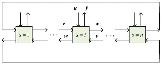
Figure 1.
Spatially interconnected systems.
In general, many physically realizable interconnected systems are only coupled with states, and the output of each subsystem is determined by its state [23,24]. Thus, this paper may as well assume that , , are all zero matrices.
Assuming that the number of subsystems is n, and have the same dimension, similarly, and are the same size. Define the following interconnection topology features [13]
Due to the non-causality of space, the interconnected systems cannot be directly analyzed by using the conventional two-dimensional system model. Therefore, it is necessary to apply “lifting technology” to transform the spatially interconnected systems into an equivalent one-dimensional dynamic model. To this end, first define the following lifting vectors
then the whole uncertain spatially interconnected systems can be described by the following model equivalently
where
It is noted that model (10) still contains interconnected variables and parameter uncertainty, so further simplification of the model is needed.
Utilizing the interconnection characteristic of (8), the relationship among interconnected variables can be written as
where is a time-independent permutation matrix.
Let , by shifting items, (10) is equivalent to the following uncertain singular interconnected systems model
where
From the causality of the singular system, it can be seen that uncertain term is non-singular for any matrix F satisfying , which implies that is also non-singular [27].
Let , construct non-singular matrices , . Make nonsingular transformation to get the equivalent system model
Since model (12) and (16) are equivalent, is also non-singular. Based on the matrix inversion formula, it can be obtained that
where
Bring (18) into (17), the relationship between state variable and interconnected variable is obtained as follows
where
By substituting (19) into (13), one-dimensional state space model of uncertain interconnected systems can be gained
where
For a simplicity of presentation, let , , , the model (20) can be reduced to the following form
3. Control Law Design
In order to design ILC law, the state space model (21) is described as an ILC structural form
means current trial of the system, indicates the finite cycle of each trial of the system.
The designed ILC law is
the current control action is equal to the previous control action plus an update item , which is calculated from the previous error information. Define the desired output trajectory , then the system tracking error vector for the k-th trial is
Introduce state error vector
for the sake of generality, assume that and , that is, system returns to the same initial state for each trial, then
and
Suppose that the update item in ILC law (23) takes the form
and , , are gain matrices to be designed, the update term is composed of state feedback information and proportional difference term of the previous output error information.
Substitute (28) into (26) and (27), let and , then the uncertain discrete repetitive process model is available
where
Hence, the stability analysis and controller synthesis of the interconnected systems will be performed next based on the discrete repetitive process model (29).
Remark 1.
Note that different learning gains in (28) correspond to different forms of ILC laws. Specifically, it can be divided into the following three categories
- 1.
- for the PD-type ILC.
- 2.
- for the P-type ILC.
- 3.
- for the D-type ILC.
4. LMI-Based Design
Lemma 3.
A discrete repetitive process described by (29) is stable along the trial if there exists matrix such that [28]
where
It should be emphasized that the inequality in Lemma 3 involves the product term of system matrix and auxiliary matrix variable S, making it difficult to directly solve the controller gain. Consequently, it needs to be transformed into linear matrix inequality through a series of transformations.
Firstly, the nominal case () is considered. The following theorem gives the LMI condition for the stability along the trial for a nominal discrete repetitive process.
Theorem 1.
Proof of Theorem 1.
By Schur’s complement lemma, (30) is transformed into
Secondly, consider the case when uncertainty arises. Theorem 2 gives the LMI condition for the robust stability of uncertain discrete repetitive process along the trial.
Theorem 2.
Proof of Theorem 2.
Left and right multiply (33) by , then make variable substitutions, let , , , , , , and therefore
It should be pointed out that the above inequality is still nonlinear due to the system uncertainty, which must be further simplified.
Note that (35) can be rewritten as
where
Then, according to Lemma 1, (36) is equivalent to
by Schur’s complement lemma, (37) can be expressed as follows
Next, left and right multiply the above inequality by , and gives
where
As mentioned earlier, left and right multiply the above inequality by , separately. Moreover, substitute for , and then (34) can be established. □
5. Simulation
To verify the feasibility, effectiveness and robustness of the proposed PD-type ILC algorithm, the active ladder circuits interconnected by four circuit units are taken as the simulation object. The interconnection structure is shown in Figure 1, where each unit referring to [29] is depicted in Figure 2.
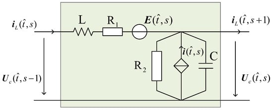
Figure 2.
Ladder circuit subunit.
The continuous model of circuit unit derived from Kirchhoff’s law is
where is continuous time, is a controlled current source dominated by voltage
parameter , inductance , capacitance , resistance , .
Take as the sampling period, and t represents the discrete time. Let the information exchanged by each subsystem be the respective inductor current and capacitor voltage, in other words, , , , .
Consequently, (40) can be discretized and rewritten as an uncertain interconnected subsystem model in the form of (5), where the state is , the input is , the output is , and the subsystem matrices are
The uncertainty of model is
parameter varies randomly within the interval , and express uncertainty in the form of (7) as
Suppose that the initial condition of the system is , finite work cycle of each trial is 6s, desired output trajectories of interconnected systems are
Meanwhile, root mean square (RMS) of tracking error is introduced as an index to evaluate the tracking performance of the interconnected systems
5.1. Nominal System
When there is no uncertainty in the system model, by utilizing Theorem 1, the gain matrices of PD-type ILC (28) are as follows
The P-type ILC is given as
and the corresponding gain matrices are
Similarly, the D-type ILC takes the form as
and the corresponding gain matrices are
The simulation results are shown in Figure 3, Figure 4 and Figure 5. With the increase of trials, the output of each subsystem asymptotically tracks to the desired reference trajectory, and the tracking error converges to zero monotonously along the trial. Besides, compared with P- and D-type ILC laws, PD-type ILC has faster convergence speed and better tracking effect, thus verifying the effectiveness and rapidity of the proposed approach.
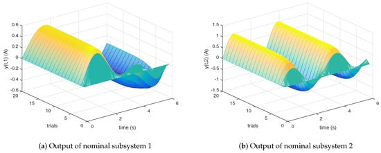
Figure 3.
Outputs of nominal subsystems 1 and 2.
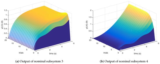
Figure 4.
Outputs of nominal subsystems 3 and 4.
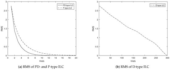
Figure 5.
RMS of PD-, P- and D-type ILC for nominal system.
5.2. Uncertain System
Consider the case when norm uncertainty is present, based on Theorem 2, the gain matrices of PD-type ILC (28) are as follows
In the same way, the gain matrices of P-type ILC (44) are
and the gain matrices of D-type ILC (45) are
As shown in Figure 6, Figure 7 and Figure 8, the simulation results indicate that the convergence rate of tracking error of the uncertain subsystems decreases significantly, but it still converges monotonously along the trial. Moreover, the convergence rate of PD-type ILC algorithm is faster than that of the P- and D-type ILC, which validates the robustness and superiority of the propounded method.

Figure 6.
Outputs of uncertain subsystems 1 and 2.
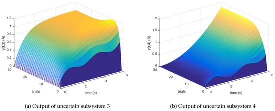
Figure 7.
Outputs of uncertain subsystems 3 and 4.
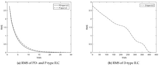
Figure 8.
RMS of PD-, P- and D-type ILC for uncertain system.
6. Conclusions
In this paper, a class of uncertain discrete spatially interconnected systems is transformed into an equivalent one-dimensional model by lifting technology and singular system theory. Based on the repetitive process theory, PD-type ILC algorithm is designed to transform the system model into discrete repetitive process model. Furthermore, the LMI conditions for the stability of nominal system and uncertain system along the trial are given. Eventually, the simulation results verify the feasibility and robustness of the algorithm.
However, there are two main limitations of the proposed methodology. Since the state feedback is used in the proposed methodology, it is not suitable for the systems whose state is not measurable. Besides, the methodology uses the lifting along the spatial variable to obtain a commonly used state-space model, the dimension of the lifting matrices will expand as the number of subsystems increases, which will lead to computational complexity. In the future, we will consider using output feedback to design ILC law and thus the application scope of the method can be extended. Furthermore, in order to reduce the scale of the control problem, it is planned to develop two-dimensional approach for spatially interconnected systems instead of lifting technology.
Author Contributions
Conceptualization, L.Z. and H.T.; methodology, V.S. and H.Y.; validation, L.Z., H.T., W.P., V.S. and H.Y.; formal analysis, L.Z. and H.T.; data curation, L.Z.; writing–original draft preparation, L.Z.; writing–review and editing, H.T., W.P. and V.S.; supervision, H.Y.; project administration, H.Y.; funding acquisition, H.T. and W.P. All authors have read and agreed to the published version of the manuscript.
Funding
This research was funded by Postgraduate Research & Practice Innovation Program of Jiangsu Province grant number KYCX20_1938, National Natural Science Foundation of China grant number 61773181,61203092, the Fundamental Research Funds for the Central Universities grant number JUSRP51733B and National Science Centre in Poland, grant No.2017/27/B/ST7/01874, the Serbian Ministry of Education, Science and Technological Development, grant No.451-03-68/2020-14/200108.
Conflicts of Interest
The authors declare no conflict of interest.
References
- Arimoto, S.; Kawamura, S.; Miyazaki, F. Bettering operation of robotics by learning. J. Robot. Syst. 1984, 1, 123–140. [Google Scholar] [CrossRef]
- Zhao, Y.M.; Lin, Y.; Xi, F.F.; Guo, S. Calibration-based iterative learning control for path tracking of industrial robots. IEEE Trans. Ind. Electron. 2015, 62, 2921–2929. [Google Scholar] [CrossRef]
- Heertjes, M.; Tso, T. Nonlinear iterative learning control with applications to lithographic machinery. Control Eng. Pract. 2007, 15, 1545–1555. [Google Scholar] [CrossRef]
- Freeman, C.T. Constrained point-to-point iterative learning control with experimental verification. Control Eng. Pract. 2012, 20, 489–498. [Google Scholar] [CrossRef]
- Tao, H.F.; Paszke, W.; Rogers, E.; Yang, H.Z.; Galkowski, K. Iterative learning fault-tolerant control for differential time-delay batch processes in finite frequency domains. J. Process Control 2017, 56, 112–128. [Google Scholar] [CrossRef]
- Hladowski, L.; Galkowski, K.; Cai, Z.L.; Rogers, E.; Freeman, C.T.; Lewin, P.L. Experimentally supported 2D systems based iterative learning control law design for error convergence and performance. Control Eng. Pract. 2010, 18, 339–348. [Google Scholar] [CrossRef]
- Paszke, W.; Rogers, E.; Galkowski, K. Experimentally verified generalized KYP Lemma based iterative learning control design. Control Eng. Pract. 2016, 53, 57–67. [Google Scholar] [CrossRef]
- Wu, F. Distributed control for interconnected linear parameter-dependent systems. IEE Proc. Control Theory Appl. 2003, 150, 518–527. [Google Scholar] [CrossRef]
- Massioni, P.; Verhaegen, M. Subspace identification of circulant systems. Automatica 2008, 44, 2825–2833. [Google Scholar] [CrossRef]
- Liu, Q.; Hoffmann, C.; Werner, H. Distributed control of parameter-varying spatially interconnected systems using parameter-dependent lyapunov functions. In Proceedings of the American Control Conference, Washington, DC, USA, 17–19 June 2013. [Google Scholar]
- Liu, H.B.; Yu, H.S. Decentralized state estimation for a large-scale spatially interconnected system. ISA Trans. 2008, 74, 67–76. [Google Scholar] [CrossRef]
- Sulikowski, B.; Gałkowski, K.; Kummert, A.; Rogers, E. Two-dimensional (2D) systems approach to feedforward/feedback control of a class of spatially interconnected systems. Int. J. Control 2018, 91, 2780–2791. [Google Scholar] [CrossRef]
- D’Andrea, R.; Dullerud, G.E. Distributed control design for spatially interconnected systems. IEEE Trans. Autom. Control 2003, 48, 1478–1495. [Google Scholar] [CrossRef]
- Fardad, M.; Jovanovic, M.R. Design of optimal controllers for spatially invariant systems with finite communication speed. Automatica 2011, 47, 880–889. [Google Scholar] [CrossRef]
- Liu, Q.; Abbas, H.S.; Mohammadpour, J.; Wollnack, S.; Werner, H. Distributed model predictive control of constrained spatially-invariant interconnected systems in input-output form. In Proceedings of the American Control Conference, Boston, MA, USA, 6–8 July 2016. [Google Scholar]
- Feng, H.Y.; Xu, H.L.; Xu, S.Y.; Chen, W.M. Model reference tracking control for spatially interconnected discrete-time systems with interconnected chains. Appl. Math. Comput. 2019, 340, 50–62. [Google Scholar] [CrossRef]
- Tao, H.F.; Paszke, W.; Yang, H.Z.; Gałkowski, K. Finite frequency range robust iterative learning control of linear discrete system with multiple time-delays. J. Franklin Inst. 2019, 356, 2690–2708. [Google Scholar] [CrossRef]
- Kim, B.Y.; Kim, Y.S.; Ahn, H.S. Stability analysis of spatially interconnected discrete-time systems with random delays and structured uncertainties. J. Franklin Inst. 2013, 350, 1719–1738. [Google Scholar] [CrossRef]
- Xu, H.L.; Lin, Z.P.; Zhai, X.K.; Feng, H.Y.; Chen, X.F. Quadratic stability analysis and robust distributed controllers design for uncertain spatially interconnected systems. J. Franklin Inst. 2018, 355, 7924–7961. [Google Scholar] [CrossRef]
- Huang, H.; Wu, Q.H. Distributed robust control of spatially interconnected systems with parameter uncertainty. In Proceedings of the IEEE Conference on Decision and Control and European Control Conference, Orlando, FL, USA, 12–15 December 2011. [Google Scholar]
- Park, G.J.; Lee, T.H.; Lee, K.H.; Hwang, K.H. Robust design: An overview. AIAA J. 2006, 44, 181–191. [Google Scholar] [CrossRef]
- Paszke, W.; Rogers, E.; Boski, M. Repetitive process based design of PD-type iterative learning control laws. In Proceedings of the Mediterranean Conference on Control and Automation, Zadar, Croatia, 19–22 June 2018. [Google Scholar]
- Jeong, J.Y.; Kim, Y.S.; Ahn, H.S. Discrete-time repetitive process-based iterative learning control for heterogeneous systems with arbitrary interconnections. In Proceedings of the IEEE International Conference on Control & Automation, Taichung, Taiwan, 18–20 June 2014. [Google Scholar]
- Kim, B.Y.; Lee, T.; Kim, Y.S.; Ahn, H.S. Iterative learning control for spatially interconnected systems. Appl. Math. Comput. 2014, 237, 438–445. [Google Scholar] [CrossRef]
- Karban, P.; Pánek, D.; Orosz, T.; Petrášová, I.; Doležel, I. FEM based robust design optimization with Agros and Ārtap. Comput. Math. Appl. 2020, 1–16. [Google Scholar] [CrossRef]
- Xie, L.H. Output feedback ∞ control of systems with parameter uncertainty. Int. J. Control 1996, 63, 741–750. [Google Scholar] [CrossRef]
- Lee, C.M.; Fong, I.K. ∞ filter design for uncertain discrete-time singular systems via normal transformation. Circ. Syst. Signal Process. 2006, 25, 525–538. [Google Scholar] [CrossRef]
- Rogers, E.; Galkowski, K.; Owens, D.H. Control Systems Theory and Applications for Linear Repetitive Processes; Springer: Berlin/Heidelberg, Germany, 2007. [Google Scholar]
- Sulikowski, B.; Gałkowski, K.; Kummert, A. Proportional plus integral control of ladder circuits modeled in the form of two-dimensional (2D) systems. Multidimens. Syst. Signal Process. 2013, 26, 267–290. [Google Scholar] [CrossRef]
© 2020 by the authors. Licensee MDPI, Basel, Switzerland. This article is an open access article distributed under the terms and conditions of the Creative Commons Attribution (CC BY) license (http://creativecommons.org/licenses/by/4.0/).