Transfer Learning for Stenosis Detection in X-ray Coronary Angiography

Abstract

Coronary artery disease is the most frequent type of heart disease caused by an abnormal narrowing of coronary arteries, also called stenosis or atherosclerosis. It is also the leading cause of death globally. Currently, X-ray Coronary Angiography (XCA) remains the gold-standard imaging technique for medical diagnosis of stenosis and other related conditions. This paper presents a new method for the automatic detection of coronary artery stenosis in XCA images, employing a pre-trained (VGG16, ResNet50, and Inception-v3) Convolutional Neural Network (CNN) via Transfer Learning. The method is based on a network-cut and fine-tuning approach. The optimal cut and fine-tuned layers were selected following 20 different configurations for each network. The three networks were fine-tuned using three strategies: only real data, only artificial data, and artificial with real data. The synthetic dataset consists of 10,000 images ($80\%$ for training, $20\%$ for validation) produced by a generative model. These different configurations were analyzed and compared using a real dataset of 250 real XCA images (125 for testing and 125 for fine-tuning), regarding their randomly initiated CNNs and a fourth custom CNN, trained as well with artificial and real data. The results showed that pre-trained VGG16, ResNet50, and Inception-v3 cut on an early layer and fine-tuned, overcame the referencing CNNs performance. Specifically, Inception-v3 provided the best stenosis detection with an accuracy of $0.95$, a precision of $0.93$, sensitivity, specificity, and $F_1$ score of $0.98$, $0.92$, and $0.95$, respectively. Moreover, a class activation map is applied to identify the high attention regions for stenosis detection.

1. Introduction

Coronary artery disease is produced by plaque buildup in the arterial walls reducing blood flow. In particular, coronary arteries exchange blood from the heart to vital parts of the human body. Such plaques are made up mainly of cholesterol and other waste products from cells. Those adipose depots cause stenosis, an unnatural narrowing of coronary arteries over time, which can partially or entirely block out the blood flow [1]. Besides, atherosclerosis is a well-known term used to describe the formation mechanism of atheromatous plaques. Coronary artery disease is the most common type of Cardiovascular Diseases (CVDs), which are the main causes of global deaths, taking out an estimated 17.9 million lives every year, according to the World Health Organization [2]. Currently, X-ray Coronary Angiography (XCA) remains the gold-standard imaging technique for the medical diagnosis of stenosis and other related conditions [1]. Noninvasive imaging methods such as Coronary Computed Tomography Angiography (CCTA) have experienced remarkable performance in detecting coronary artery stenosis. However, XCA performs best for high-grade stenosis or severe calcifications, it is also possible to identify almost all the coronary arterial vessels [3]. For clinical purposes, if the physician finds a significant blockage in one of the blood vessels during the XCA, an immediate angioplasty can clear the blockage, in contrast to a CCTA. These two main screening exams require an injection of dye and radiation exposure. In XCA procedure, a liquid dye, such as fluorescein, is injected using a thin catheter inserted into an access point to the bloodstream (usually in the arm or groin). The dye reveals an arterial structure that can be easily seen on X-ray images and allows cardiovascular technicians to detect narrowed or blocked areas through coronary arteries. In Figure 1. X-ray coronary angiograms with stenosis regions are illustrated.

In clinical practice, the specialists perform an exhaustive visual examination over the X-ray angiogram for detecting this kind of abnormalities. However, given the limited access to such delicate clinical expertise, the variability of diagnoses among specialists, have allowed that the automatic Computer-Aided Diagnosis (CAD) systems play a vital role in cardiology to detect coronary artery stenosis. In literature, several methods for detecting coronary stenosis in XCA images have been commonly addressed concerning vessel detection (enhancement), vessel segmentation, and vessel skeletonization. Kishore and Jayanthi [4] proposed a method for stenosis detection based on a manually selected fixed-size window (patch) from the enhanced image to lastly apply an adaptive threshold segmentation algorithm. From this segmented and cropped vessel region, the vessel width (that determines the percentage of stenosis and its grading), was calculated by adding the intensity values from the left to the right edge with no need for a skeletonization process. Saad [5] applied a skeletonization process after segmenting to obtain the vessel centerline and compute the orthogonal line’s length as the vessel width of a fixed-size window moving through it. The vessel width allows determining if stenosis exists.

On the other hand, the candidate stenosis regions are selected by the Hessian matrix after the binarization and skeletonization steps. Thus, Sameh et al. [6] used a Hessian-based vessel enhancement to identify narrowed arteries areas. A binary image is generated from these predefined areas, and the artery lumen is afterwards computed. Alternatively, Wan et al. [7] carried out the vessel diameter estimation using a smoothed vessel centerline curve from the candidate stenosis regions detected by the Hessian approach. Previous artery lumen/vessel diameter estimation allows determining stenosis measurement and final classification. Cervantes-Sanchez et al. [8] proposed a method for computing the vessel width along the arteries by applying the second-order derivatives directly over the enhanced images. The cases of stenosis were labeled as local minima through the vessel width. addIn this approach, no additional skeletonization or vessel diameter estimation was needed. Posteriorly, Cruz-Aceves et al. [9] used a Bayes classifier over a handcrafted 3D feature vector hemhat was obtained from the results of potential cases of coronary stenosis identified previously by a second-order derivative operator.

On the other hand, Convolutional Neural Networks (CNNs) have succeeded as a method to automatically learn and estimate a set of discriminant features directly from raw data at multiple abstractions for accurate classification [10]. Furthermore, CNNs have been successfully used in diverse application areas in medical imaging such as image enhancement, segmentation, lesion localization, and classification [11]. It is noteworthy that CNNs are characterized by an intrinsic transferability of knowledge embedded in the pre-trained CNNs. Azizpour et al. [12] suggest that the success of knowledge transfer depends on dissimilarity between the source domain (where the CNN has trained) and the target domain (where the knowledge is transferred). Despite the dissimilarity between natural and medical imaging, recent studies have shown the potential for transfer learning to the medical imaging domain, such as chest imaging [13,14], breast imaging [15,16], and retinal imaging [17].

In the context of coronary stenosis detection in XCA images, Antczak and Liberadzki [18] developed a patch-based CNN based on four convolutional layers and one dense layer, trained from scratch using random weights initialization. Each convolutional layer has a $7\times 7$ kernel size. Besides, a dropout layer is applied after the 1st, 3rd, and fourth layer. This approach employed an artificial dataset to overcome the problem of limited training data. Afterward, a tuning stage is carried out using patches from real XCA images to improve network accuracy. Likewise, Au et al. [19] trained from scratch a small patch-based CNN for stenosis detection, constituted by five convolutional layers with a kernel size pattern of $3\times 3$ followed by a $1\times 1$ until reaching five layers, a single global max pooling, and one dense layer.

Moreover, data augmentation techniques (e.g., random shift, random rotation, and random shear) were applied during the training phase. Cong et al. [20] employed a pre-trained Inception-V3 [21] network replacing the last fully convolutional layers with custom classification layers for a binary stenosis classification setup. Only the appended layers were trained while keeping the remainder of the network unchanged. This approach takes advantage of a rich sequence of XCA images to improve training and reduce overfitting, which adds redundant frames to the training process. More recently, Wu et al. [22] proposed a CNN-based method to achieve automatic and accurate stenosis detection, with temporal constraints on the XCA sequence. First candidate frames for stenosis detection were selected, such that the segmented vascular area is maximum. Next, a deconvolutional single-shot detector [23] in a VGG19 (with 19 convolutional layers) is applied to conduct stenosis detection directly on the selected raw X-ray angiograms. Finally, the method exploits the potential temporal consistency of the selected frames to remove false positives detections.

In this paper, a new method for automatic detection of coronary artery stenosis in XCA images, employing a pre-trained CNN via Transfer Learning (VGG16, ResNet50, and Inception-v3) is proposed. The proposed method incorporates a network-cut approach were the layers between the cut layer and the initial layer of the custom classifier are discarded to reduce the number of transferred layers of each network. Hence, the number of parameters that the architecture will have to fine-tune decreases as well. Furthermore, the network performance is improved by fine-tuning in a layer-wise manner in the chopped network. The optimal cut and fine-tuned layers were selected following twenty different configurations for each network. These different configurations were analyzed and compared in terms of five different evaluation metrics. The proposed method showed that cut and fine-tuning a pre-trained CNN in a layer-wise manner improves the performance against CNNs trained from scratch. The presented results were obtained using three fine-tuning strategies: (1) using only real data, (2) using only artificial data, and (3) with a composed tuning of artificial and real data. The artificial dataset contains 10,000 artificial XCA images ($80\%$ for fine-tuning and $20\%$ for validation). The real dataset consists of 250 real XCA images, where 125 are used for additional fine-tuning (third fine-tuning strategy), and the remained 125 images for testing. This two-stage fine-tuning (artificial with real data) allows improving the detection results when the networks were randomly initialized. It also provides a slight improvement for pre-trained network initialization against random initialized with only real data fine-tuning. The remainder of this document is organized as follows: Section 2 briefly describes the concepts related to convolutional neural networks and transfer learning. Section 3 presents the proposed methodology for stenosis detection. In Section 4, the experimental results are shown and discussed. Finally, the conclusions are drawn in Section 5.

2. Background

In this section, the basis of Convolutional Neural Networks, VGG16, ResNet50, and Inception-v3 networks employed in this study are described in Section 2.1. Additionally, Transfer Learning is detailed in Section 2.2.

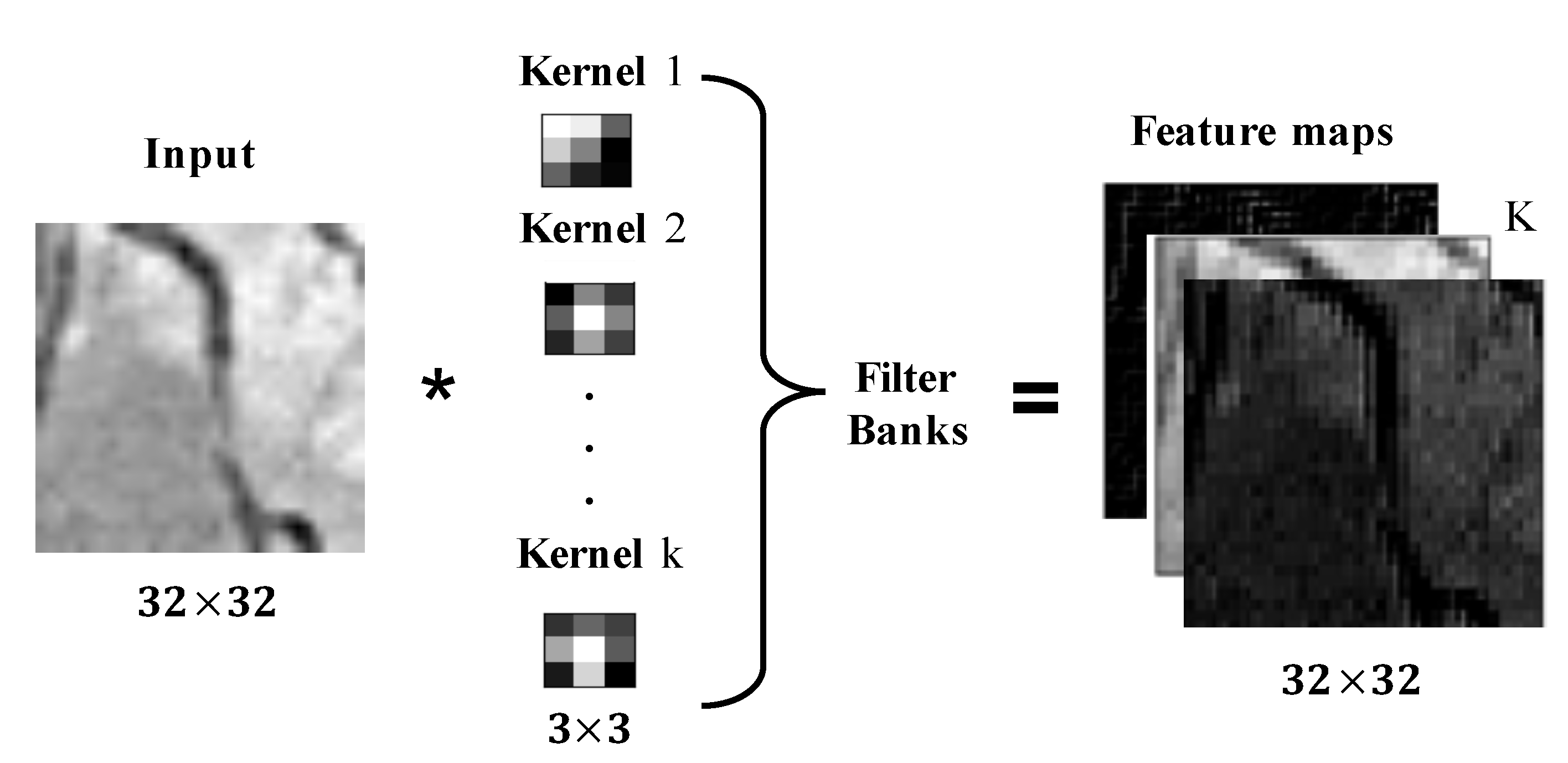
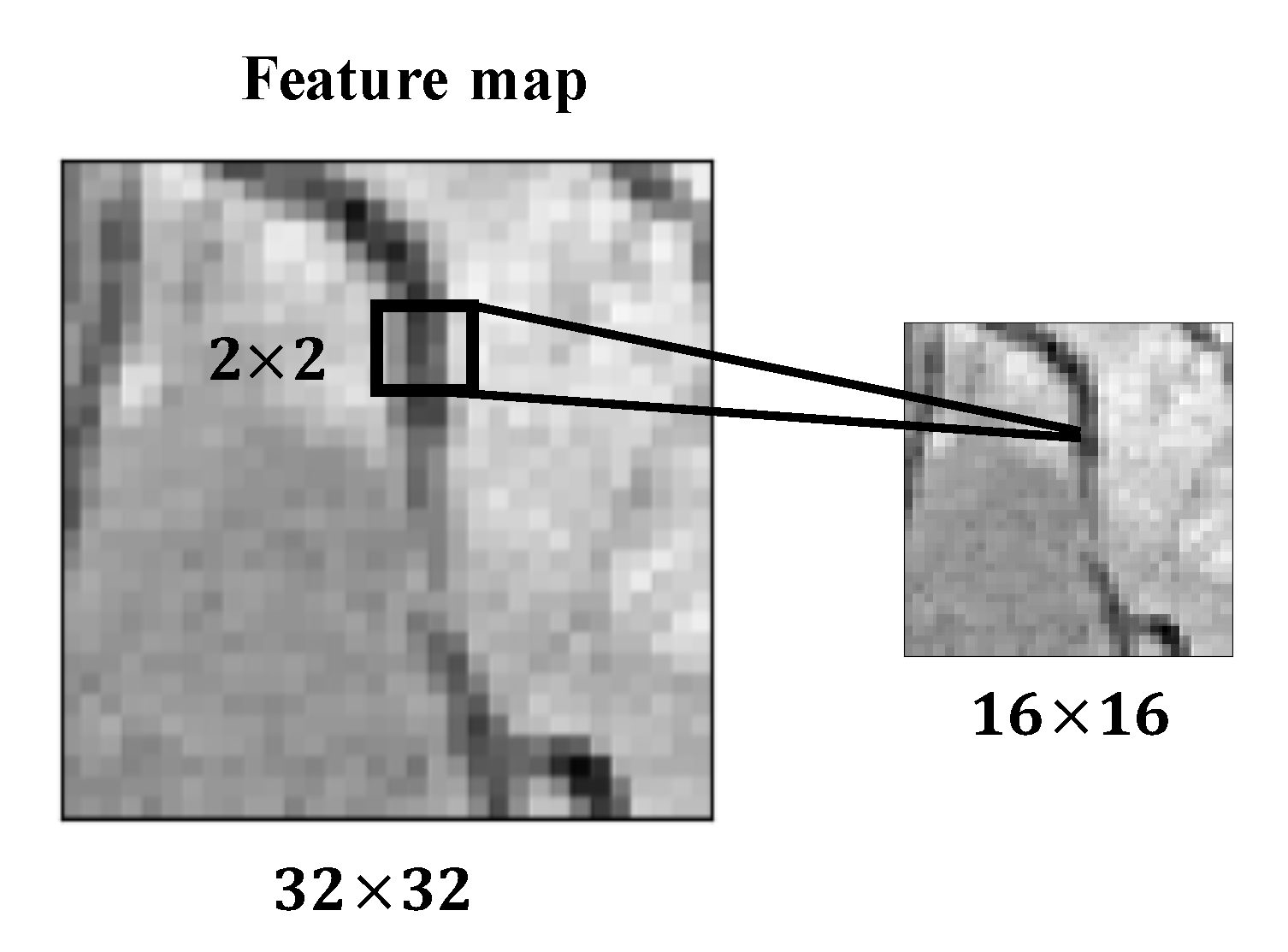
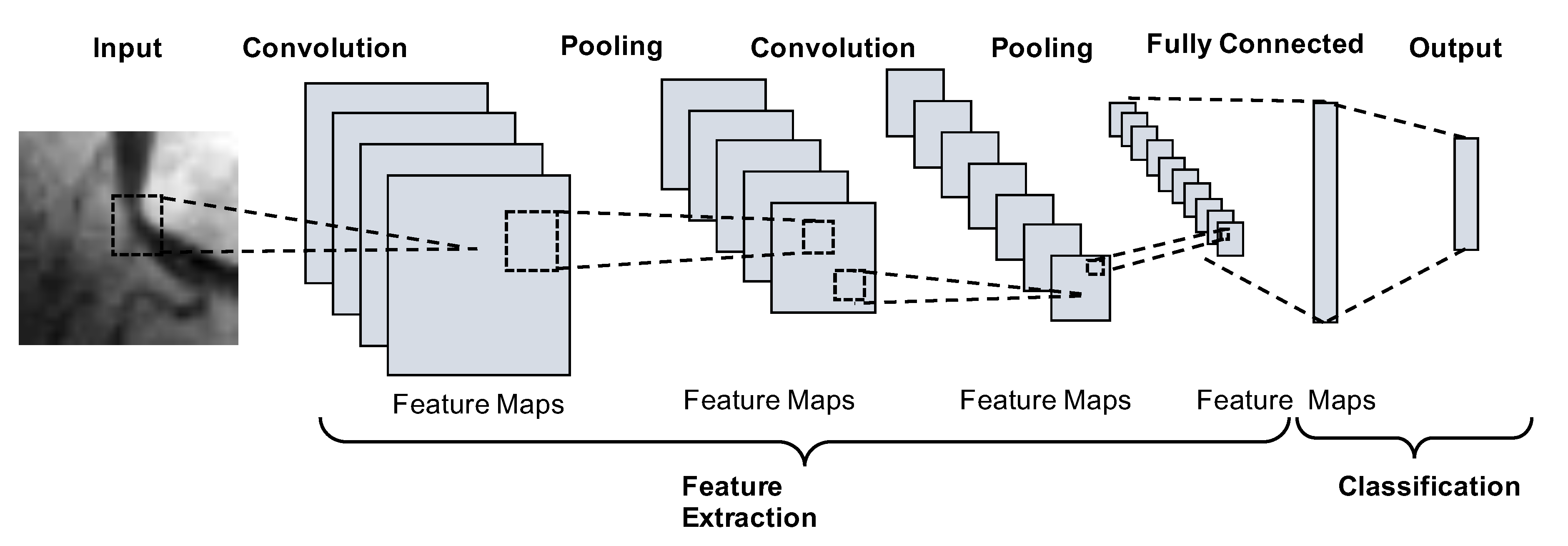
2.1. Convolutional Neural Networks

The core of Convolutional Neural Networks (CNNs) are layers that can extract local features (e.g., edges) across a set of input images through convolution kernels. These layers are known as convolutional layers. They can be viewed as 2-D filters (kernels), which are represented by matrices. Hence, the convolution outcome is also known as a feature map. Thus, a convolutional layer with K kernels is trained to detect K local features whose strength across the input images is visible in the resulting K feature maps, as is illustrated in Figure 2.

Each feature map ${\mathbf{O}}_k$ is mathematically described by

$${\mathbf{O}}_k=\sum _n{\mathbf{W}}_k\left[n\right]\ast \mathbf{I}\left[n\right],$$

(1)

where $\mathbf{I}\left[n\right]$ is the n-th input channel, ${\mathbf{W}}_k\left[n\right]$ is the sub-kernel for such a channel and * is the convolution operator.

Likewise, to reduce computational complexity and prevent over-fitting, each convolutional layer sequence is followed by a pooling layer (i.e., down-sampling layer). Indeed, the pooling operation reduces the dimension of the output neurons of the convolutional layer. The max-pooling layer is the most commonly used configuration, which reduces the size of feature maps by selecting the maximum feature response in each feature map sequence. This process is formally given as follows:

$${\mathbf{H}}_k[i,j]=\underset{p}{arg\; max}{\mathbf{O}}_k[i+p,j+p],$$

(2)

where p is the pooling size and determines the max-pooling window size. In Figure 3, the max-pooling operation is illustrated.

In Figure 4, an underlying CNN architecture is introduced. The design typically consists of several pairs of convolutional and pooling layers (feature extraction), followed by consecutive fully connected layers (classification) using every neuron of the previous layer connected to the next layer neurons. Finally, the last activation function is used to generate the output classification labels.

In this work, VGG16, ResNet50, and Inception-v3, three state-of-the-art networks represent some of the highest performing CNNs on the ImageNet Large Scale Visual Recognition Challenge (ILSVR) [24] competition over the past few years were studied. These networks also demonstrate a strong ability to generalize to medical imaging via transfer learning, such as feature extraction and fine-tuning.

The VGG [25] architecture was proposed by the Oxford Visual Geometry Group and used to win the ILSVR competition in 2014. The fundamental idea behind this architecture is to increase the network depth by adding more convolutional layers while keeping unchanged the other tuning parameters. The VGG family, instead of having several hyperparameters, is focused on disposing of small convolution layers of $3\times 3$ filters with a stride of 1 pixel. After working on the block of convolutional layers, a max-pooling operation is performed over a $2\times 2$ filter using, in this case, a stride of 2 pixels. The VGG-16 has 16 convolutional layers starting with 64 feature maps per layer and increasing up to 512 feature maps. Two fully-connected layers, each with 4096 nodes, are then followed by a softmax classifier.

The ResNet [26] family introduces a residual connection to the model. A residual connection allows skipping to process a few layers. ResNet only has one fully-connected layer with 1000 neurons, which produce the output class probabilities. This residual connection goes directly over the next layer, improving the learning process. The ResNet50 (with a total of 50 convolutional layers) network consists of five major blocks. The first one is composed of a convolutional and a pooling layer. In contrast, the remainder blocks contain a stack of 3, 4, 6, and 3 layers, comprising convolutional filters of different depth and size ($1\times 1$, $3\times 3$, and $1\times 1$). Besides, the $1\times 1$ layers are responsible for reducing and afterward increasing (restoring) the feature maps dimension. Convolutional layers and pooling layers work with a stride of 2 pixels. These residual blocks contain convolutional layers starting with 64 feature maps until obtaining 2048 feature maps.

Inception-v3 [21] is a CNN with 48 convolutional layers, which classifies images into 1000 object classes. This architecture introduces three distinct types of Inception modules (A, B, and C) to reduce the number of connections/parameters without decreasing network efficiency. In Inception module A, two $3\times 3$ convolutions replace one $5\times 5$ convolution, in Inception module B, one $3\times 1$ convolution followed by one $1\times 3$ convolution replace one $3\times 3$ convolution, and in Inception module C, one $1\times 7$ and $7\times 1$ convolution replace one $7\times 7$ convolution. The output feature maps of each Inception module are 288, 768, and 2048, respectively.

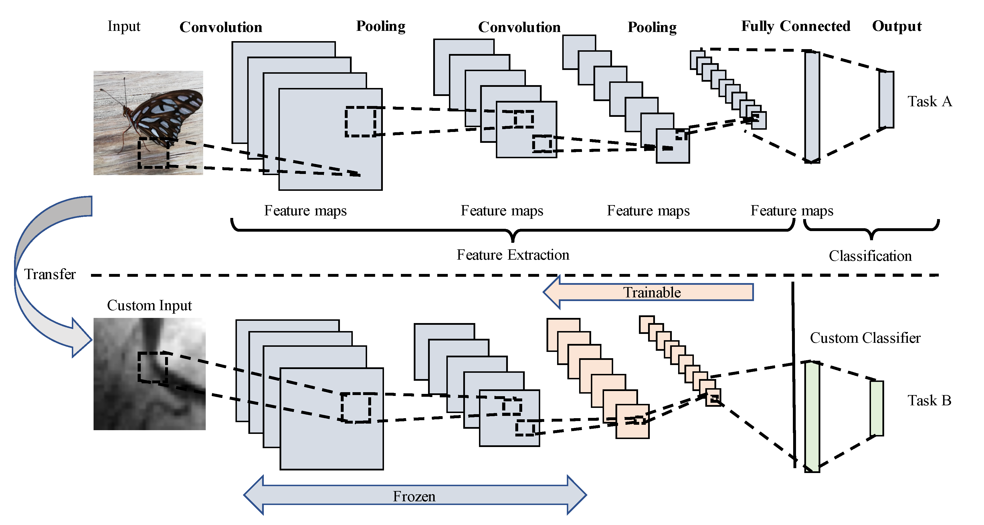
2.2. Transfer Learning

CNNs are generally trained through backpropagation, where the unknown network weights are updated in each iteration by minimizing a specific cost function. Typically, the weights are initialized with a random set of values. However, this kind of initialization requires a high number of training samples; for instance, ImageNet is a dataset that contains 14 million images with over 1000 classes [27]. An alternative to the randomized weights initialization is the transfer learning strategy. Transfer learning begins by transferring the weights from a pre-trained network (source domain) to the actual network that is desired to train (target domain) [28,29]. A common practice consists of replacing the last fully-connected layer of the pre-trained CNN with a new fully-connected layer having the same number of neurons that the number of classes for the specific problem at hand, as shown in Figure 5.

In fact, training a CNN from a set of pre-trained weights is called fine-tuning. After the weights of the last fully connected layers have been initialized, the new network can be fine-tuned in a layer-wise manner. Fine-tuning the last few layers is usually enough for transfer learning, which means changing the weights during the gradient descent optimization. Despite the dissimilarity between the source and the target domain increases, the fine-tuning at first layers must be employed to learn more generic features from the target domain [30]. Therefore, the features extracted from low-level layers are more generic (e.g., luminance, edges, contrasted colors, and curves) than top-layers. Furthermore, the features appear not specific to a particular dataset or task, while features extracted from top-layers are more defined to the classes of a given task.

3. Proposed Method for Stenosis Detection

The proposed method for stenosis detection is discussed in this section. The network-cut and fine-tuning approach as well as the proposed classifier and hyperparameter selection, are described in Section 3.1 and Section 3.2. Later, a class activation map is introduced in Section 3.3, and finally, the metrics used to evaluate stenosis detection performance can be found in Section 3.4.

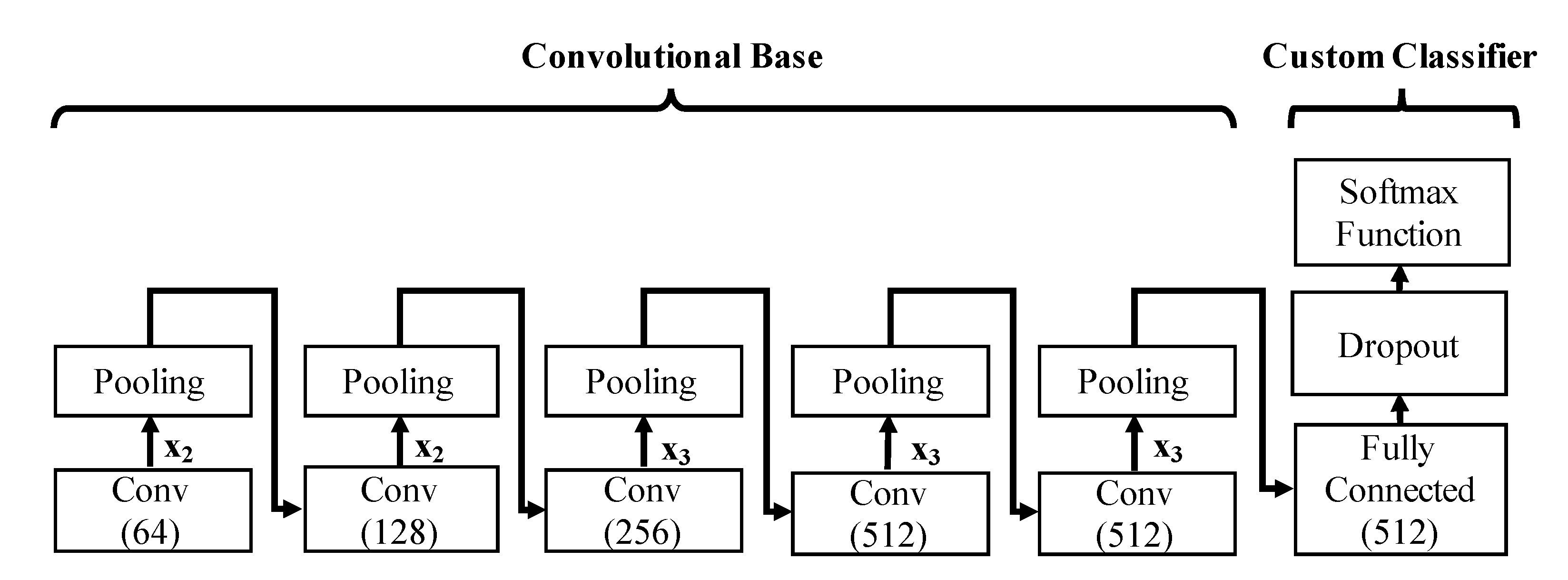
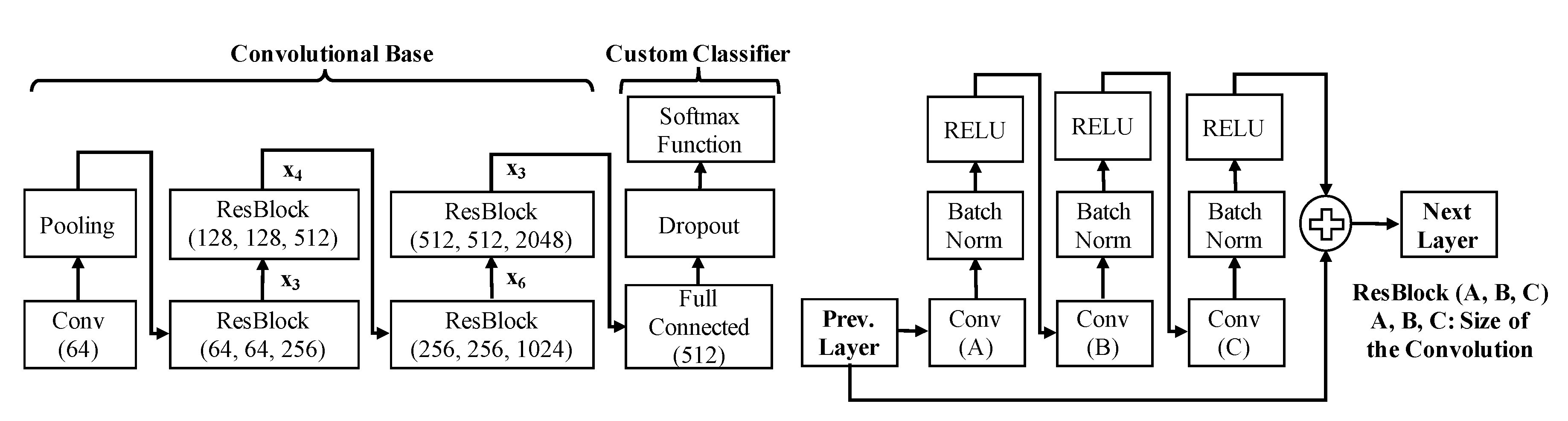
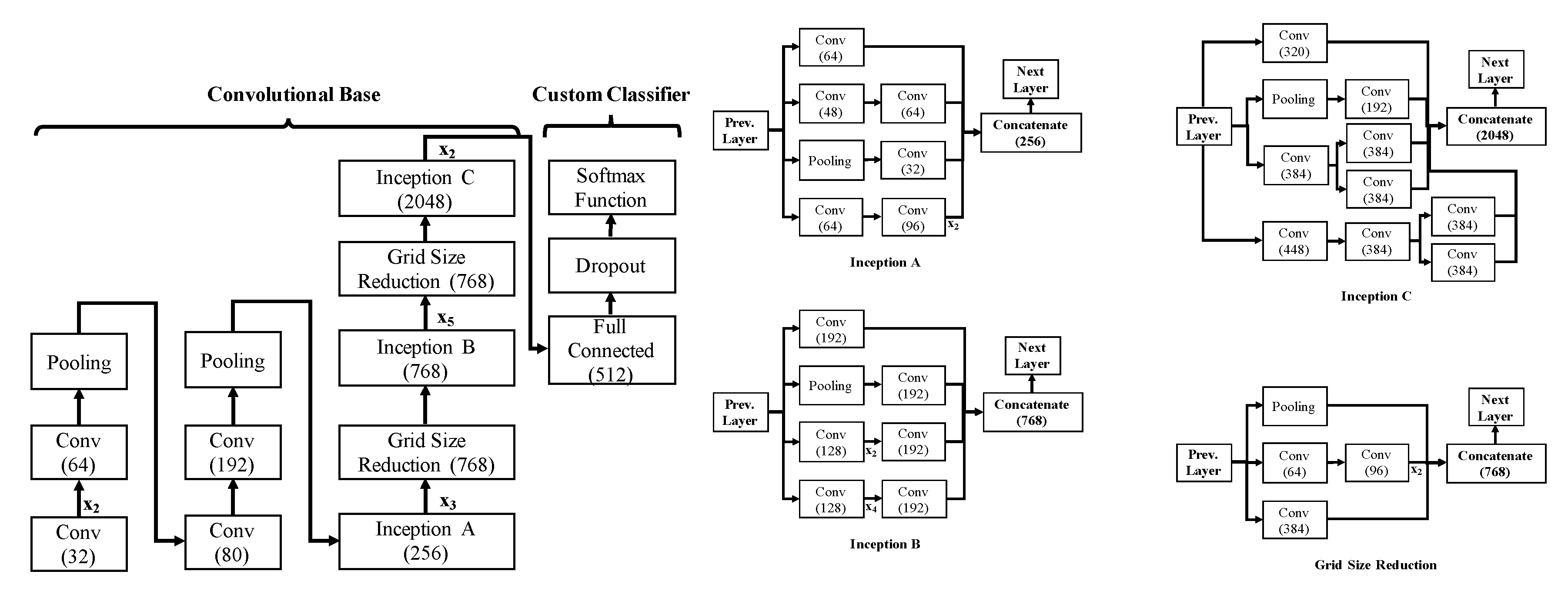
3.1. Network Architecture

According to the dissimilarity of the source and target domains, additional layers must be fine-tuned starting from the last layer. The precedent extra layers are incrementally included in the update process. However, this fine-tuning scheme might not reach the desired performance due to the depth dimension of the pre-trained CNN. In this study, a network-cut approach is introduced, where the pre-trained network output can be extracted from an early layer (i.e., layers between the cut layer and the initial layer of the custom classifier are discarded) to improve the network performance. Figure 6 shows an outline of the fine-tuning stage and the network cut methodology.

The best cut and frozen layers are repeatedly achieved until the desired learning performance is reached. The fine-tuning and network-cut strategies allow us to transfer and fine-tune only the most discriminant features, reducing the network size (therefore, the number of layers) while maintaining the learning performance improvement. In this work, a 3-layer classifier is proposed, which is composed of a fully connected layer with 512 neurons, followed by a dropout regularization layer [31]. In the output layer, the activation values of the regularization layer are processed into a sigmoid function. Such a process guarantees that network output is always in the interval $[0,1]$ to detect stenosis diagnosis. The neuronal weights of the classification layers are initialized with the algorithm described in [32] as

$${\mathbf{W}}_k\sim U\left(-1/\sqrt{m},1/\sqrt{m}\right),$$

(3)

where $U(-a,b)$ is a uniform distribution in the interval $[-a,b]$, and m is the size of the previous layer. Indeed, the main goal of network training is to maximize the probability of obtaining an accurate classification. As all optimization processes, learning is achieved by minimizing an objective function. In this case, the cross-entropy loss function was chosen to evaluate the fitting of each training sample. The loss function is defined as follows:

$$L\left(\mathbf{W}\right)=-\frac{1}{N}\sum _{n=1}^N\left(y_{n}log\left({\widehat{y}}_n\right)+(1-y_n)log(1-{\widehat{y}}_n)\right),$$

(4)

where y is the ground-truth label for a given input patch that belongs to $[0,1]$, respectively labeled as non-stenosis or stenosis on a given patch. $\widehat{y}$ represents the predicted probability (predicted label) of the n-th patch estimated directly by the CNN, and N is the number of samples. The loss function is minimized during the model training process by computing the gradient of the function L with respect to the network weights $\mathbf{W}$. It is noteworthy that during this process, the pre-trained weights $\mathbf{W}$ that in the model were set to trainable mode (unfreeze), are updated using the stochastic gradient descent (SGD) algorithm. Therefore, the SGD method is mathematically described by

$$\begin{array}{cc}\hfill {\mathbf{V}}_{k+1}& =\mu {\mathbf{V}}_k-\sigma \nabla L\left({\mathbf{W}}_k\right),\hfill \\ \hfill {\mathbf{W}}_{k+1}& ={\mathbf{W}}_k+{\mathbf{V}}_{k+1},\hfill \end{array}$$

(5)

where ${\mathbf{W}}_k$ stands for weight parameters in the CNN at iteration k, and $\nabla L\left({\mathbf{W}}_k\right)$ is the gradient of the loss function at iteration k. Likewise, when calculating the gradient $\nabla L\left({\mathbf{W}}_k\right)$, only a batch of N samples are used for avoiding to process all data [33]. $\mathbf{V}$ is the integrated velocity initialized at zero, $\mu$ is the momentum coefficient to use a temporally averaged gradient to boost the optimization velocity, and $\sigma$ is the learning rate. Three pre-trained architectures on the ImageNet dataset (VGG16, ResNet50, and Inception-v3) were the neural networks used to test the network-cut and fine-tuning methodologies. The pre-trained networks were fine-tuned using a batch size $N=100$, a maximum of 1000 epochs, a fixed momentum $\mu =0.9$, and an initial learning rate of $\sigma =1e^{-3}$. If the validation loss ($VL$) is not improving during $\tau$ epochs, the learning rate is decreased (until reaching a minimum of $\sigma =5e^{-7}$) given the following expression:

$$\sigma =\left\{\begin{array}{cc}\sigma \ast \sqrt{0.1}\hfill & V{L}_e\ge V{L}_{e+\tau },\hfill \\ \sigma \hfill & \mathrm{otherwise},\hfill \end{array}\right.$$

(6)

where $V{L}_e$ and $V{L}_{e+\tau }$ are the validation loss at epochs e and $e+\tau$, respectively. Furthermore, early stopping was employed to reduce overfitting and the computational cost of the training procedure. The algorithm terminates when the validation loss has not improved over 500 epochs, keeping the model with the best validation loss.

Figure 7 presents the architecture of the first transfer learning model. Such an architecture closely follows the VGG16 architecture; the fully connected layers are only changed for the proposed 3-layer classifier.

The architecture of the second transfer learning model is shown in Figure 8. This model is based on a ResNet50 architecture, like the VGG16 transfer learning model, the last fully connected layers were adjusted by the custom classifier.

At last, the Inception-v3 architecture using the custom classification layers for stenosis detection is shown in Figure 9.

3.2. Network Configuration

In the proposed method, the cut layer used at the end of the fine-tuned layer of the pre-trained network is carried out in descending and progressive way. Each network is divided into six blocks of layers. In total, a set of 20 different network configurations for VGG16, ResNet50, and Inception-v3 were analyzed. These settings progressively cut and fine-tune the network layer blocks one at a time. The blocks and layers to test the proposed network-cut and fine-tuning approach in the VGG16 neural architecture are given in

Table 1. VGG16 Network: block structure and convolutional layers grouping.

Block Number	Convolutional Layers
1	{1, 2}
2	{3, 4}
3	{5, 6, 7}
4	{8, 9, 10}
5	{11, 12, 13}
6	Fully Connected Layers (Classifier)

.

The different network configurations for ResNet50 follow the layers grouping and blocks given in

Table 2. ResNet50 network: block structure and convolutional layers grouping.

Block Number	Description	Convolutional Layers
1	Convolutional Layer	{1}
2	Residual blocks	{1, 2, 3}
3		{4, 5, 6, 7}
4		{9, 10, …, 13}
5		{14, 15, 16}
6	Fully Connected Layers	Classifier

.

For Inception-v3 CNN, the layer grouping and blocks are detailed in

Table 3. Inception-v3 network: block structure and convolutional layers grouping.

Block Number	Description	Convolutional Layers
1	Convolutional Layer	{1, 2, 3}
2		{4, 5}
3	Inception blocks	{1, 2, 3}
4		{4, 5, …, 8}
5		{9, 10, 11}
6	Fully Connected Layers	Classifier

.

From these configurations, the cut and froze block layers were studied. Accordingly, four characteristic behaviors can be distinguished from these network configurations:

• Feature extractor: The entire pre-trained CNN is idle, whereas the weights of the pre-trained convolutional layers remain fixed, and only the fully connected layers are trained with the selected dataset, as in [20].
• Fine-tuning: The whole network is fine-tuned in a layer-wise manner from top to low-level blocks, where the blocks of convolutional layers pass to trainable on a descendent way. In this behavior, the number of convolutional trainable blocks is increased from one to five convolutional blocks, while the fully connected layers are always included in the training.
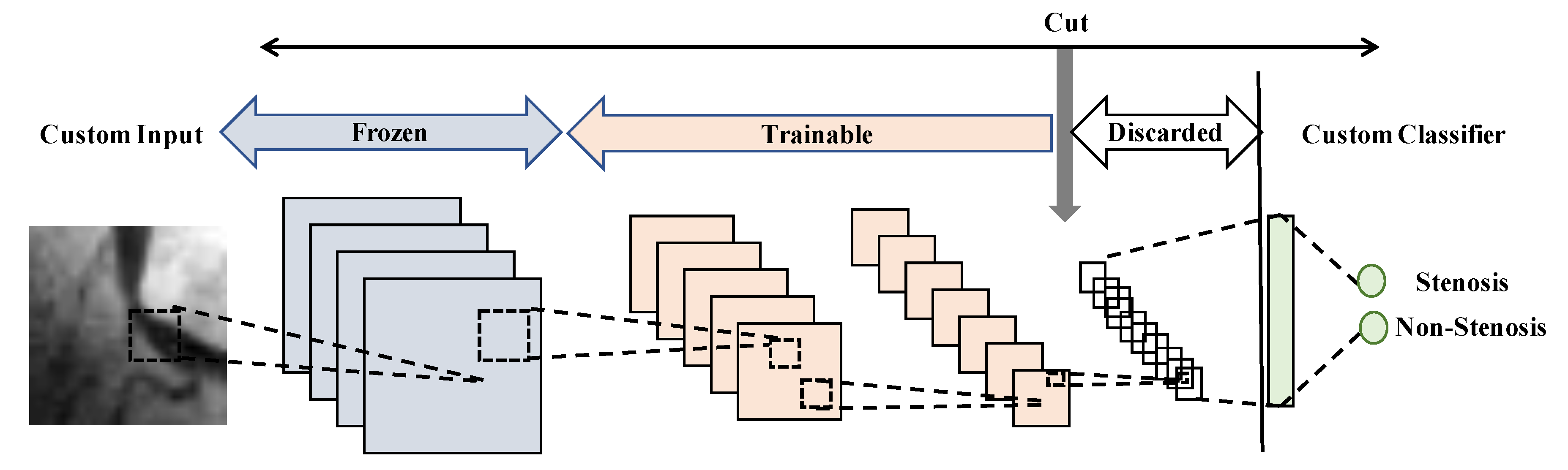
• Network-cut and feature extractor: the network is chopped up on an early convolutional block, retaining their weights. Then from this block, the last fully connected layer and softmax activation layer are added and trained. Notice that the layers after the cut block are discarded.
• Network-cut and fine-tuning: the network is chopped up on an early convolutional block, but a fine-tuning process is carried out in a layer-wise manner from new top-layers to low-level layers, as well as the fully connected layers.

In those architecture behaviors, the proposed configuration exploits the network-cut approach, performing the fine-tuning on the new top-layers simultaneously. The tested network configurations are given in

Table 4. The 20 network configurations applied to VGG16, ResNet50, and Inception-v3, respectively. N/A: Not applicable.

Cut Block	Fine-Tuned Blocks
N/A	{6}
	{5, 6}
	{4, 5, 6}
	{3, 4, 5, 6}
	{2, 3, 4, 5, 6}
	{1, 2, 3, 4, 5, 6}
4	{6}
	{4, 6}
	{3, 4, 6}
	{2, 3, 4, 6}
	{1, 2, 3, 4, 6}
3	{6}
	{3, 6}
	{2, 3, 6}
	{1, 2, 3, 6}
2	{6}
	{2, 6}
	{1, 2, 6}
1	{6}
	{1, 6}

. On the other hand, in the cases when the network was trained from scratch (random weights initialization), only the second and the fourth behavior will apply, which means that the full or a chopped network are trainable.

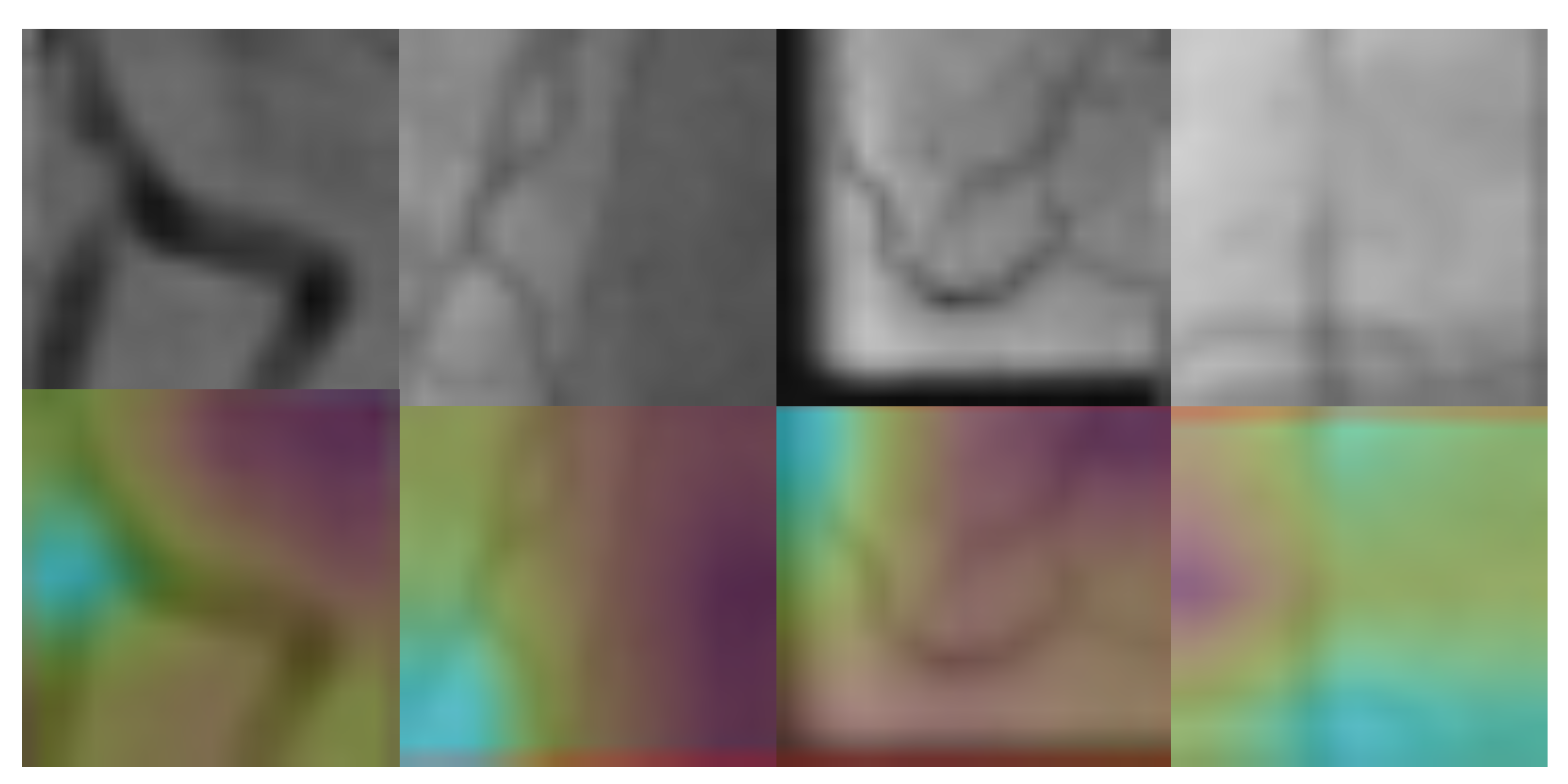
3.3. Stenosis Activation Maps

After stenosis classification, a class activation map (Grad-CAM [34]) is applied to produce a coarse localization map highlighting the image’s discriminant regions for a specific detected class. The Grad-CAM calculation is described as a linear addition of K feature maps ${\mathbf{O}}_k$ in a layer l and their weights ${\mathbf{W}}_k\left[s\right]$ into a specific class (stenosis). These feature maps are then spatially pooled using a Global Average Pooling (GAP) to produce the score $\mathbf{M}\left[s\right]$ as follows:

$$\mathbf{M}\left[s\right]=\frac{1}{Z}\sum _i\sum _j\sum _k{\mathbf{W}}_k\left[s\right]{\mathbf{O}}_k[i,j],$$

(7)

where Z is a normalization factor. In the proposed model, $s=1$ is chosen due to the output layer (activated by a sigmoid function) returns a single value, and layer l is taken as the final convolutional layer.

3.4. Evaluation Metrics

In this study, five binary metrics were used for precisely measuring the performance of the classification algorithms. Those metrics include accuracy, sensitivity (recall), specificity, precision, and $F_1$-score. Accuracy (ACC) is defined as the ratio of the correctly classified instances over the total number of instances, which is formally defined as

$$Accuracy=\frac{TP+TN}{TP+TN+FP+FN},$$

(8)

where TP (true positive) is the number of positive instances (stenosis cases) that are correctly classified. TN (true negative) is the number of negative instances (no-stenosis cases) that are correctly classified, and FP (false positive) and FN (false negative) are respectively the numbers of positive and negative instances that are incorrectly classified, concerning a ground-truth.

Sensitivity (SN), also known as the true positive rate or recall, measures the fraction of correctly classified positive instances as follows,

$$Sensitivity\left(Recall\right)=\frac{TP}{TP+FN}.$$

(9)

Specificity (SP), or the true negative rate, measures the fraction of correctly classified negative instances, which is given by

$$Specificity=\frac{TN}{TN+FP}.$$

(10)

Precision (PC), or positive predictive value, measures the fraction of positive instances that are correctly classified. Such a metric is formally defined as follows

$$Precision=\frac{TP}{TP+FP}.$$

(11)

A general F-score metric arises combining the precision and recall measures, which is described as follows

$$F_{\beta }=(1+{\beta }^2)\frac{Precision\times Recall}{{\beta }^{2}Precision+Recall}.$$

(12)

In particular, a balanced F-score is obtained when $\beta =1$, thus such expression is well-known as the $F_1$ measure.

4. Results and Discussion

The fine-tuning of the proposed method was evaluated using three different strategies: (1) using only real data, (2) using only the artificial dataset, and (3) using artificial data and an additional fine-tuning using real data. The classification results for each fine-tuned strategy are presented. Moreover, in this section, a comparative analysis of the proposed network-cut and fine-tuning approach for stenosis detection are included. The analysis was made concerning the pre-trained networks VGG16, ResNet50, and Inception-v3 based on the five binary classification metrics’ results. The computational experiments were implemented on a Cloud Platform disposing of an Intel(R) Xeon(R) CPU, 12 GB of RAM, and 2.00 GHz dual-processor. The GPU Platform was based on a Tesla P4 having 2560 CUDA cores and 8 GB VRAM. The experiments were developed with Python 3.6, Keras 2.3.1, and TensorFlow 2.2.0-rc3.

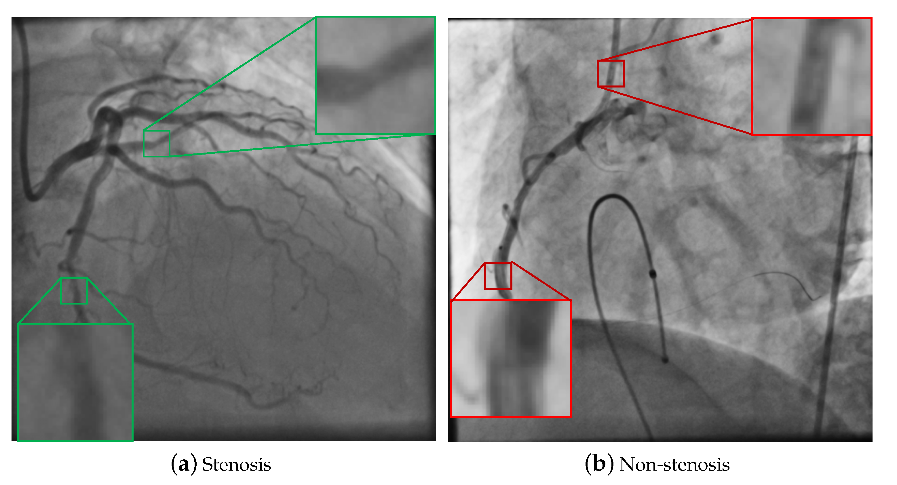
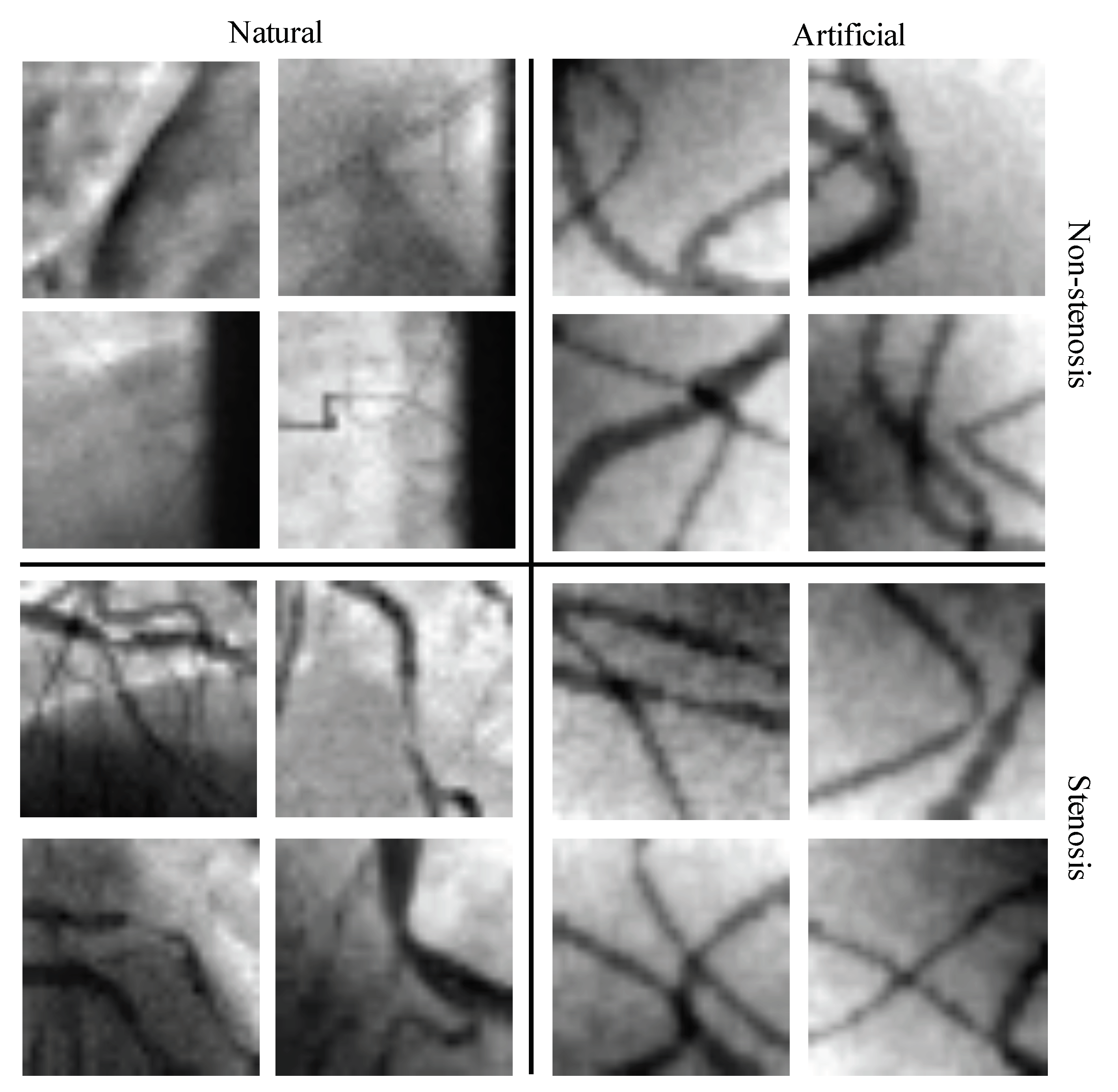
4.1. Databases of Coronary Stenosis

Antczak and Liberadzki [18] introduced two datasets to train, validate, and test a CNN for stenosis detection; the datasets are publicly available on the GitHub platform [35]. The first dataset consists of 10,000 gray-scale artificial patches of $32\times 32$ pixels, $50\%$ of data contain stenosis cases and remainder data are considered as no-stenosis. This dataset employs an artificial data generator that produces a set of artificial patches assuming that patches from angiographic images can be modeled with Bézier curves of various lengths and widths to represent the real blood vessels.

The second dataset contains 250 real XCA images, with 125 patches identified with stenosis and 125 with no-stenosis. In the numerical experiments, the only required pre-processing was a straightforward scale normalization changing the pixel intensities linearly from $[0,255]$ to $[0,1]$ interval. Figure 10 shows some real and artificial patches used in the learning process.

Note that there may be multiple patches classified as stenosis, even if there is one stenosis per XCA image due to the patch overlapping process. In the first fine-tuning strategy, only real data was employed. The real dataset was split into 100, 25, 125 data for fine-tuning (training), validation, and testing sets, respectively. The second and third strategy randomly split the artificial dataset into $80\%$ of data for fine-tuning (training) and $20\%$ for validation. From the real data, $50\%$ was used as a testing set. Additionally, the third strategy takes the remaining $50\%$ of real data for additional fine-tuning.

4.2. Network-Cut and Fine-Tuning

Twenty different configurations of each pre-trained networks were explored to determine the optimal network-cut and fine-tuning blocks for each fine-tuning strategy. Additionally, these configurations were tested using a random initialization (trained from scratch). The best-obtained configurations: full network as features extractor (FNFE), full network and fine-tuning (FNFT), network-cut as features extractor (NCFE), and network-cut and fine-tuning (NCFT) in terms of validation function loss are presented in

Table 5. The best neural network configurations applied to VGG16, ResNet50, and Inception-v3 were analyzed by two weights initializations: ImageNet and random (trained from scratch).

Network	Initialization	Fine-Tuning Strategy	Best Configuration	Cut Block	Fine-Tuned Blocks
VGG16	Random	Only real data	FNFE	N/A	N/A
			FNFT	N/A	{1, 2, …, 6}
			NCFE	N/A	N/A
			NCFT	2	{1, 2, 6}
		Only artificial data	FNFE	N/A	N/A
			FNFT	N/A	{1, 2, …, 6}
			NCFE	N/A	N/A
			NCFT	2	{1, 2, 6}
		Artificial + real data	FNFE	N/A	N/A
			FNFT	N/A	{1, 2, …, 6}
			NCFE	N/A	N/A
			NCFT	1	{1, 6}
VGG16	ImageNet	Only real data	FNFE	N/A	{6}
			FNFT	N/A	{1, 2, …, 6}
			NCFE	4	{6}
			NCFT	3	{2, 6}
		Only artificial data	FNFE	N/A	{6}
			FNFT	N/A	{4, 5, 6}
			NCFE	3	{6}
			NCFT	3	{1, 2, 3, 6}
		Artificial + real data	FNFE	N/A	{6}
			FNFT	N/A	{2, 3, …, 6}
			NCFE	4	{6}
			NCFT	3	{3, 6}
ResNet50		Only real data	FNFE	N/A	N/A
			FNFT	N/A	{1, 2, …, 6}
			NCFE	N/A	N/A
			NCFT	2	{1, 2, 6}
		Only artificial data	FNFE	N/A	N/A
			FNFT	N/A	{1, 2, …, 6}
			NCFE	N/A	N/A
			NCFT	2	{1, 2, 6}
		Artificial + real data	FNFE	N/A	N/A
			FNFT	N/A	{1, 2, …, 6}
			NCFE	N/A	N/A
			NCFT	4	{1, 2, 3, 4, 6}
	ImageNet	Only real data	FNFE	N/A	{6}
			FNFT	N/A	{1, 2, …, 6}
			NCFE	3	{6}
			NCFT	2	{1, 2, 6}
		Only artificial data	FNFE	N/A	{6}
			FNFT	N/A	{5, 6}
			NCFE	3	{6}
			NCFT	2	{1, 2, 6}
		Artificial + real data	FNFE	N/A	{6}
			FNFT	N/A	{1, 2, …, 6}
			NCFE	2	{6}
			NCFT	2	{1, 2, 6}
Inception-v3	Random	Only real data	FNFE	N/A	N/A
			FNFT	N/A	{1, 2, …, 6}
			NCFE	N/A	N/A
			NCFT	3	{1, 2, 3, 6}
		Only artificial data	FNFE	N/A	N/A
			FNFT	N/A	{1, 2, …, 6}
			NCFE	N/A	N/A
			NCFT	2	{1, 2, 6}
		Artificial + real data	FNFE	N/A	N/A
			FNFT	N/A	{1, 2, …, 6}
			NCFE	N/A	N/A
			NCFT	2	{1, 2, 6}
	ImageNet	Only real data	FNFE	N/A	{6}
			FNFT	N/A	{1, 2, …, 6}
			NCFE	3	{6}
			NCFT	3	{1, 2, 3, 6}
		Only artificial data	FNFE	N/A	{6}
			FNFT	N/A	{3, 4, 5, 6}
			NCFE	3	{6}
			NCFT	3	{2, 3, 6}
		Artificial + real data	FNFE	N/A	{6}
			FNFT	N/A	{1, 2, …, 6}
			NCFE	3	{6}
			NCFT	3	{1, 2, 3, 6}

.

As mentioned before, in the cases when the network was trained from scratch (random weights initialization), only the full network with fine-tuning and network-cut with fine-tuning configuration was applied. The analysis suggests that the VGG16 network maintains 1 and 2 blocks in case of random initialization; on the other hand, the pre-trained VGG16 keeps 3- and 4-layer blocks. The best cut-block among the different ResNet50 configurations was achieved using 2 and 4 blocks for a randomly initialized settings; oppositely, employing the pre-trained weights, the best settings maintain 2 and 3 blocks. In the case of the Inception-v3 network, the network-cut was on the 2nd and third block for random and pre-trained initialization, respectively.

4.3. Detection Results

In this study, the analysis of the proposed network-cut approach was carried out using three state-of-the-art architectures: VGG16 [25], ResNet50 [26], and Inception-v3 [21]. Each architecture was evaluated using two network initializations: random and pre-trained weights and employing three different fine-tuning strategies: only real data, only artificial, and a combination of synthetic with real data. Additionally, a custom CNN proposed by Antczak and Liberadzki [18] for stenosis detection was taken as a baseline measurement.

Table 6. Network detection results. The testing set of 125 real XCA patches was used to evaluate the detection performance for each best neural network configuration applied to VGG16, ResNet50, and Inception-v3 with the weights initialization: ImageNet and random (trained from scratch).

Network	Initialization	Fine-Tuning Strategy	Best Configuration	Detection Performance
				ACC	PC	SN	${\mathbf{F}}_1$	SP
Antczak and Liberadzki [18]	Random	Only real data	FNFT	0.60	0.60	0.66	0.63	0.53
		Only artificial data	FNFT	0.59	0.55	0.87	0.68	0.33
		Artificial + real data	FNFT	0.89	0.87	0.90	0.89	0.88
VGG16 [25]	Random	Only real data	FNFE	N/A	N/A	N/A	N/A	N/A
			FNFT	0.55	0.53	0.86	0.66	0.24
			NCFE	N/A	N/A	N/A	N/A	N/A
			NCFT	0.50	0.50	1.00	0.67	0.00
		Only artificial data	FNFE	N/A	N/A	N/A	N/A	N/A
			FNFT	0.52	0.53	0.40	0.45	0.65
			NCFE	N/A	N/A	N/A	N/A	N/A
			NCFT	0.51	0.52	0.41	0.46	0.61
		Artificial + real data	FNFE	N/A	N/A	N/A	N/A	N/A
			FNFT	0.54	0.55	0.46	0.50	0.61
			NCFE	N/A	N/A	N/A	N/A	N/A
			NCFT	0.50	0.52	0.25	0.34	0.76
	ImageNet	Only real data	FNFE	0.87	0.85	0.90	0.88	0.84
			FNFT	0.93	0.91	0.95	0.93	0.90
			NCFE	0.92	0.91	0.94	0.92	0.90
			NCFT	0.92	0.90	0.95	0.92	0.89
		Only artificial data	FNFE	0.70	0.69	0.71	0.70	0.68
			FNFT	0.58	0.56	0.84	0.67	0.32
			NCFE	0.53	0.52	0.73	0.61	0.32
			NCFT	0.63	0.58	0.94	0.72	0.32
		Artificial + real data	FNFE	0.87	0.85	0.90	0.88	0.84
			FNFT	0.91	0.87	0.97	0.92	0.85
			NCFE	0.89	0.86	0.94	0.89	0.84
			NCFT	0.94	0.91	0.97	0.94	0.90
ResNet50 [26]	Random	Only real data	FNFE	N/A	N/A	N/A	N/A	N/A
			FNFT	0.46	0.45	0.32	0.37	0.61
			NCFE	N/A	N/A	N/A	N/A	N/A
			NCFT	0.82	0.77	0.94	0.84	0.71
		Only artificial data	FNFE	N/A	N/A	N/A	N/A	N/A
			FNFT	0.52	0.52	0.63	0.57	0.40
			NCFE	N/A	N/A	N/A	N/A	N/A
			NCFT	0.48	0.49	0.70	0.58	0.26
		Artificial + real data	FNFE	N/A	N/A	N/A	N/A	N/A
			FNFT	0.86	0.83	0.90	0.86	0.81
			NCFE	N/A	N/A	N/A	N/A	N/A
			NCFT	0.83	0.84	0.83	0.83	0.84
	ImageNet	Only real data	FNFE	0.50	0.00	0.00	0.00	1.00
			FNFT	0.79	0.77	0.84	0.80	0.74
			NCFE	0.91	0.88	0.95	0.92	0.87
			NCFT	0.91	0.88	0.95	0.92	0.87
		Only artificial data	FNFE	0.52	0.56	0.22	0.32	0.82
			FNFT	0.55	0.55	0.62	0.58	0.48
			NCFE	0.66	0.69	0.57	0.63	0.74
			NCFT	0.71	0.68	0.83	0.74	0.60
		Artificial + real data	FNFE	0.50	0.00	0.00	0.00	1.00
			FNFT	0.90	0.93	0.87	0.90	0.94
			NCFE	0.75	0.92	0.56	0.69	0.95
			NCFT	0.91	0.89	0.94	0.91	0.89
Inception-v3 [21]	Random	Only real data	FNFE	N/A	N/A	N/A	N/A	N/A
			FNFT	0.51	1.00	0.03	0.06	1.00
			NCFE	N/A	N/A	N/A	N/A	N/A
			NCFT	0.71	0.70	0.75	0.72	0.68
		Only artificial data	FNFE	N/A	N/A	N/A	N/A	N/A
			FNFT	0.47	0.48	0.62	0.54	0.32
			NCFE	N/A	N/A	N/A	N/A	N/A
			NCFT	0.58	0.58	0.67	0.62	0.50
		Artificial + real data	FNFE	N/A	N/A	N/A	N/A	N/A
			FNFT	0.82	0.78	0.90	0.84	0.74
			NCFE	N/A	N/A	N/A	N/A	N/A
			NCFT	0.94	0.91	0.97	0.94	0.90
	ImageNet	Only real data	FNFE	0.88	0.82	0.98	0.89	0.77
			FNFT	0.57	0.60	0.43	0.50	0.71
			NCFE	0.95	0.93	0.98	0.95	0.92
			NCFT	0.92	0.90	0.95	0.92	0.89
		Only artificial data	FNFE	0.49	0.49	0.51	0.50	0.47
			FNFT	0.38	0.41	0.49	0.45	0.27
			NCFE	0.69	0.64	0.87	0.74	0.50
			NCFT	0.63	0.58	0.94	0.72	0.32
		Artificial + real data	FNFE	0.73	0.77	0.65	0.71	0.81
			FNFT	0.88	0.90	0.86	0.88	0.90
			NCFE	0.87	0.94	0.79	0.86	0.95
			NCFT	0.94	0.95	0.92	0.94	0.95

presents stenosis detection performance rates of each best configuration of random and pre-trained CNN architecture evaluated in the subset of 125 real XCA patches in terms of accuracy, precision, recall, $F_1$-score, and specificity. For each fine-tuning strategy and network initialization, the best performance was highlighted. According to Table 6, the random-initialized networks with only real or artificial data for fine-tuning resulted in reduced accuracy, reaching a maximum of $0.55$, $0.82$, and $0.71$ on the VGG16, ResNet50, and Inception-v3 architectures, respectively. Furthermore, attempting to improve the detection performance of the random initialized networks, during the fine-tuning, a strategy of combining artificial and real data was carried on, reaching an accuracy of $0.54$, $0.83$, and $0.94$ with the VGG16, ResNet50, and Inception-v3 architectures, respectively. It is noteworthy that the Inception-v3 architecture presents the best improvement, outperforming the accuracy obtained by Antczak and Liberadzki [18]. On the other hand, by using pre-trained networks, the use of only real data surpasses the use of only artificial data for fine-tuning, reaching an accuracy of $0.93$, $0.91$, and $0.95$ for VGG16, ResNet50, and Inception-v3, respectively. By employing the combination of artificial and real data for fine-tuning, the VGG16 accuracy improves to $0.94$, while ResNet50 and Inception-v3, maintained their performances.

Finally, it is noteworthy that the proposed method, including both the network-cut and fine-tuning of a pre-trained network for stenosis detection, achieved better results against the network-cut at some specific block, and keep the weights unchanged. Thus, the accuracy improvement regarding the referencing random weighted initialization CNN proposed by Antczak and Liberadzki [18] is attained using the three pre-trained VGG16, ResNet50, and Inception-v3 networks. In the case of VGG16, the best accuracy was obtained using only three blocks with fine-tuning, ResNet50 employed and fine-tuned the first two blocks of layers, and for Inception-v3, the three top blocks are maintained and keep idle (no fine-tuning needed).

A class activation map was obtained to get a visual explanation for the areas where the image features have the most significant impact on prediction. Figure 11 shows the case examples of predictions using the best predictive model obtained from the network-cut and fine-tuned approaches. The best-performing CNN model was pre-trained Inception-v3 fine-tuned with only real data. Each case example employed a Grad-CAM technique to perform a visual interpretation to determine which features activate the last convolutional layer more intensely before the classification. As one can see, in the case of correct detection (true positive and true negative), CNN is identifying prominent features located in the vessel pixels (regions in light green or yellow). Meanwhile, in the case of incorrect detection (false positive and false negative), the CNN identify background pixels as high attention regions, i.e., the non-stenosis case predicted as stenosis. However, in the false-positive case, some regions displayed in purple (low attention) corresponds to vessel pixels. These images provide valuable information about the localization of features that has the most significant impact on the prediction stage.

5. Conclusions

In this paper, a network-cut and fine-tuning hybrid method for stenosis detection in XCA images was introduced. The extensive numerical experiments, based on 20 distinct setups for the pre-trained (on the ImageNet dataset) and randomly initialized with three different fine-tuning strategies for the VGG16, ResNet50, and Inception-v3 networks were implemented. They have demonstrated that employing a pre-trained network on a limited XCA dataset performs efficiently for stenosis detection. For the pre-trained networks, the obtained results showed that the fine-tuning required to achieve the best accuracy was to apply fine-tuning in all remained layers for VGG16 and ResNet50, and with no-fine-tuning for Inception-v3. The proposed scheme allowed an accuracy improvement respect to the network configurations trained from scratch. Furthermore, the numerical findings allowed asserting that fine-tuning with artificial and real data approach improves the performance and accuracy of the VGG16 model for stenosis detection. The pre-trained Inception-v3 with only the three top blocks as feature extractor reaches an accuracy of $0.95$, precision of $0.93$, sensitivity of $0.98$, $F_1$-score of $0.95$, and specificity of $0.92$ for stenosis detection. Besides, a class activation map using the Grad-CAM technique was performed to a deep learning-based visual explanation for the areas where the image features have the most significant impact on prediction. A limitation of this study is a particular implementation using patched-based stenosis detection. The accuracy results reached in this paper could be further improved by adding a more sophisticated generative model for obtaining simulated data and incorporating an image-level detection approach. Finally, according to the numerical and visual results, the proposed method consisting of network-cut and fine-tune a pre-trained network (specifically regarding the Inception-v3 architecture) has shown the potential to detect coronary stenosis, that performed with high accuracy for computer-aided diagnosis in cardiology.

References

1. Athanasiou, L.S.; Fotiadis, D.I.; Michalis, L.K. Atherosclerotic Plaque Characterization Methods Based on Coronary Imaging; Academic Press: Cambridge, MA, USA, 2017. [Google Scholar]
2. World Health Organization. Cardiovascular Diseases (CVDs). 2020. Available online: https://www.who.int/news-room/fact-sheets/detail/cardiovascular-diseases-(cvds) (accessed on 30 August 2020).
3. Eckert, J.; Schmidt, M.; Magedanz, A.; Voigtländer, T.; Schmermund, A. Coronary CT angiography in managing atherosclerosis. Int. J. Mol. Sci. 2015, 16, 3740–3756. [Google Scholar] [CrossRef] [PubMed]
4. Kishore, A.N.; Jayanthi, V. Automatic stenosis grading system for diagnosing coronary artery disease using coronary angiogram. Int. J. Biomed. Eng. Technol. 2019, 31, 260–277. [Google Scholar] [CrossRef]
5. Saad, I.A. Segmentation of Coronary Artery Images and Detection of Atherosclerosis. J. Eng. Appl. Sci. 2018, 13, 7381–7387. [Google Scholar] [CrossRef]
6. Sameh, S.; Azim, M.A.; AbdelRaouf, A. Narrowed Coronary Artery Detection and Classification using Angiographic Scans. In Proceedings of the 2017 12th International Conference on Computer Engineering and Systems (ICCES), Cairo, Egypt, 19–20 December 2017; pp. 73–79. [Google Scholar]
7. Wan, T.; Feng, H.; Tong, C.; Li, D.; Qin, Z. Automated Identification and Grading of Coronary Artery Stenoses with X-ray Angiography. Comput. Methods Programs Biomed. 2018, 167, 13–22. [Google Scholar] [CrossRef] [PubMed]
8. Cervantes-Sanchez, F.; Cruz-Aceves, I.; Hernandez-Aguirre, A. Automatic detection of coronary artery stenosis in X-ray angiograms using Gaussian filters and genetic algorithms. In AIP Conference Proceedings; AIP Publishing LLC: Melville, NY, USA, 2016; Volume 1747, p. 020005. [Google Scholar]
9. Cruz-Aceves, I.; Cervantes-Sanchez, F.; Hernandez-Aguirre, A. Automatic Detection of Coronary Artery Stenosis Using Bayesian Classification and Gaussian Filters Based on Differential Evolution. In Hybrid Intelligence for Image Analysis and Understanding; Wiley: Hoboken, NJ, USA, 2017; pp. 369–390. [Google Scholar]
10. LeCun, Y.; Bengio, Y.; Hinton, G. Deep learning. Nature 2015, 521, 436–444. [Google Scholar] [CrossRef] [PubMed]
11. Litjens, G.; Kooi, T.; Bejnordi, B.E.; Setio, A.A.A.; Ciompi, F.; Ghafoorian, M.; Van Der Laak, J.A.; Van Ginneken, B.; Sánchez, C.I. A survey on deep learning in medical image analysis. Med. Image Anal. 2017, 42, 60–88. [Google Scholar] [CrossRef] [PubMed] [Green Version]
12. Azizpour, H.; Sharif Razavian, A.; Sullivan, J.; Maki, A.; Carlsson, S. From Generic to Specific Deep Representations for Visual Recognition. In Proceedings of the IEEE Conference on Computer Vision and Pattern Recognition Workshops, Boston, MA, USA, 7–12 June 2015; pp. 36–45. [Google Scholar]
13. Yadav, S.S.; Jadhav, S.M. Deep convolutional neural network based medical image classification for disease diagnosis. J. Big Data 2019, 6, 113. [Google Scholar] [CrossRef] [Green Version]
14. Xu, S.; Wu, H.; Bie, R. CXNet-m1: Anomaly Detection on Chest X-Rays With Image-Based Deep Learning. IEEE Access 2018, 7, 4466–4477. [Google Scholar] [CrossRef]
15. Shen, L.; Margolies, L.R.; Rothstein, J.H.; Fluder, E.; McBride, R.; Sieh, W. Deep Learning to Improve Breast Cancer Detection on Screening Mammography. Sci. Rep. 2019, 9, 1–12. [Google Scholar] [CrossRef] [PubMed]
16. Wu, J.; Peck, D.; Hsieh, S.; Dialani, V.; Lehman, C.D.; Zhou, B.; Syrgkanis, V.; Mackey, L.; Patterson, G. Expert identification of visual primitives used by CNNs during mammogram classification. In Medical Imaging 2018: Computer-Aided Diagnosis; International Society for Optics and Photonics: Bellingham, WA, USA, 2018; Volume 10575, p. 105752T. [Google Scholar]
17. Chakravarthy, A.D.; Abeyrathna, D.; Subramaniam, M.; Chundi, P.; Halim, M.S.; Hasanreisoglu, M.; Sepah, Y.J.; Nguyen, Q.D. An Approach Towards Automatic Detection of Toxoplasmosis using Fundus Images. In Proceedings of the 2019 IEEE 19th International Conference on Bioinformatics and Bioengineering (BIBE), Athens, Greece, 28–30 October 2019; pp. 710–717. [Google Scholar]
18. Antczak, K.; Liberadzki, Ł. Stenosis Detection with Deep Convolutional Neural Networks. In MATEC Web of Conferences; EDP Sciences: Ullis, France, 2018; Volume 210, p. 04001. [Google Scholar]
19. Au, B.; Shaham, U.; Dhruva, S.; Bouras, G.; Cristea, E.; Coppi, A.; Warner, F.; Li, S.X.; Krumholz, H. Automated Characterization of Stenosis in Invasive Coronary Angiography Images with Convolutional Neural Networks. arXiv 2018, arXiv:1807.10597. [Google Scholar]
20. Cong, C.; Kato, Y.; Vasconcellos, H.D.; Lima, J.; Venkatesh, B. Automated Stenosis Detection and Classification in X-ray Angiography Using Deep Neural Network. In Proceedings of the 2019 IEEE International Conference on Bioinformatics and Biomedicine (BIBM), San Diego, CA, USA, 18–21 November 2019; pp. 1301–1308. [Google Scholar]
21. Szegedy, C.; Liu, W.; Jia, Y.; Sermanet, P.; Reed, S.; Anguelov, D.; Erhan, D.; Vanhoucke, V.; Rabinovich, A. Going deeper with convolutions. In Proceedings of the IEEE Conference on Computer Vision and Pattern Recognition, Boston, MA, USA, 7–12 June 2015; pp. 1–9. [Google Scholar]
22. Wu, W.; Zhang, J.; Xie, H.; Zhao, Y.; Zhang, S.; Gu, L. Automatic detection of coronary artery stenosis by convolutional neural network with temporal constraint. Comput. Biol. Med. 2020, 118, 103657. [Google Scholar] [CrossRef] [PubMed]
23. Fu, C.Y.; Liu, W.; Ranga, A.; Tyagi, A.; Berg, A.C. Dssd: Deconvolutional single shot detector. arXiv 2017, arXiv:1701.06659. [Google Scholar]
24. Russakovsky, O.; Deng, J.; Su, H.; Krause, J.; Satheesh, S.; Ma, S.; Huang, Z.; Karpathy, A.; Khosla, A.; Bernstein, M.; et al. ImageNet Large Scale Visual Recognition Challenge. Int. J. Comput. Vis. 2015, 115, 211–252. [Google Scholar] [CrossRef] [Green Version]
25. Simonyan, K.; Zisserman, A. Very Deep Convolutional Networks for Large-Scale Image Recognition. In Proceedings of the 3rd International Conference on Learning Representations, ICLR 2015, San Diego, CA, USA, 7–9 May 2015. [Google Scholar]
26. He, K.; Zhang, X.; Ren, S.; Sun, J. Deep Residual Learning for Image Recognition. In Proceedings of the IEEE Conference on Computer Vision and Pattern Recognition, Las Vegas, NV, USA, 27–30 June 2016; pp. 770–778. [Google Scholar]
27. Deng, J.; Dong, W.; Socher, R.; Li, L.J.; Li, K.; Fei-Fei, L. ImageNet: A Large-Scale Hierarchical Image Database. In Proceedings of the 2009 IEEE Conference on Computer Vision and Pattern Recognition, Miami, FL, USA, 20–25 June 2009; pp. 248–255. [Google Scholar]
28. Yosinski, J.; Clune, J.; Bengio, Y.; Lipson, H. How transferable are features in deep neural networks? In Proceedings of the Advances in Neural Information Processing Systems, Montreal, QC, Canada, 8–13 December 2014; pp. 3320–3328. [Google Scholar]
29. Oh, K.; Chung, Y.C.; Kim, K.W.; Kim, W.S.; Oh, I.S. Classification and Visualization of Alzheimer’s Disease using Volumetric Convolutional Neural Network and Transfer Learning. Sci. Rep. 2020, 10, 18150. [Google Scholar] [CrossRef] [PubMed] [Green Version]
30. Tajbakhsh, N.; Shin, J.Y.; Gurudu, S.R.; Hurst, R.T.; Kendall, C.B.; Gotway, M.B.; Liang, J. Convolutional Neural Networks for Medical Image Analysis: Full Training or Fine Tuning? IEEE Trans. Med. Imaging 2016, 35, 1299–1312. [Google Scholar] [CrossRef] [PubMed] [Green Version]
31. Srivastava, N.; Hinton, G.; Krizhevsky, A.; Sutskever, I.; Salakhutdinov, R. Dropout: A Simple Way to Prevent Neural Networks from Overfitting. J. Mac. Learn. Res. 2014, 15, 1929–1958. [Google Scholar]
32. Glorot, X.; Bengio, Y. Understanding the difficulty of training deep feedforward neural networks. In Proceedings of the Thirteenth International Conference on Artificial Intelligence and Statistics, Sardinia, Italy, 13–15 May 2010; pp. 249–256. [Google Scholar]
33. Krizhevsky, A.; Sutskever, I.; Hinton, G.E. ImageNet Classification with Deep Convolutional Neural Networks. In Proceedings of the Advances in Neural Information Processing Systems, Lake Tahoe, NV, USA, 3–6 December 2012; pp. 1097–1105. [Google Scholar]
34. Selvaraju, R.R.; Cogswell, M.; Das, A.; Vedantam, R.; Parikh, D.; Batra, D. Grad-CAM: Visual Explanations from Deep Networks via Gradient-based Localization. In Proceedings of the IEEE International Conference on Computer Vision, Venice, Italy, 22–29 October 2017; pp. 618–626. [Google Scholar]
35. Antczak, K.; Liberadzki, Ł. Deep Stenosis Detection Dataset. 2020. Available online: https://github.com/KarolAntczak/DeepStenosisDetection (accessed on 30 August 2020).
Figure 1. X-ray coronary angiography images. (a) The visible stenosis regions are marked in green, and (b) the non-stenosis regions are marked in red.
Mathematics 08 01510 g001
Figure 2. Illustration of a module of convolutional layers and the output feature maps. A 32 × 32 input image is convolved with a set of 3 × 3 kernels to obtain K feature maps. The number of pixels that filters shift out over the input image is called the stride (here, a stride of 1 was used).
Mathematics 08 01510 g002
Figure 3. Operation of max-pooling layer block. A 2 × 2 max-pooling operation follows the 32 × 32 K feature maps. The stride parameter was fixed to 1.
Mathematics 08 01510 g003
Figure 4. The architecture of a typical Convolutional Neural Network (CNN).
Mathematics 08 01510 g004
Figure 5. Transfer learning scheme. The last fully-connected layers are replaced with custom layers for the proposed problem. The fine-tuning is carried out in the top-level layers, while the rest of the transfer networks remains temporarily idle or frozen (i.e., the weights stay unchanged during the optimization process).
Mathematics 08 01510 g005
Figure 6. Outline of the fine-tuning stage and network cut methodology. The top-layers are discarded. At the same time, the next middle-layers are set to train. The low-layers are idle (no under training).
Mathematics 08 01510 g006
Figure 7. Architecture of the VGG16 Network.
Mathematics 08 01510 g007
Figure 8. Architecture of the ResNet50 Network.
Mathematics 08 01510 g008
Figure 9. Architecture of the Inception-v3 Network.
Mathematics 08 01510 g009
Figure 10. Natural and artificial samples from stenosis datasets. Left images are real patches from X-ray Coronary Angiography (XCA), and the right-side images are the artificial patches. The upper-side sampled patches with non-stenosis, and the lower-side are positives cases of stenosis.
Mathematics 08 01510 g010
Figure 11. Raw XCA and Grad-class activation map (CAM) sample images of correctly and incorrectly predicted stenosis by the best-performing deep Convolutional Neural Network (CNN) model (pre-trained Inception-v3 fine-tuned with only real images). Left to right: true positive, true negative, false positive, and false negative. Below each raw sample images, a Grad-CAM image is blended over the original. Regions in light green or yellow indicate the region that has the most significant impact on prediction.
Mathematics 08 01510 g011