Feasibility of Automatic Seed Generation Applied to Cardiac MRI Image Analysis

Abstract

We present a method of using interactive image segmentation algorithms to reduce specific image segmentation problems to the task of finding small sets of pixels identifying the regions of interest. To this end, we empirically show the feasibility of automatically generating seeds for GrowCut, a popular interactive image segmentation algorithm. The principal contribution of our paper is the proposal of a method for automating the seed generation method for the task of whole-heart segmentation of MRI scans, which achieves competitive unsupervised results (0.76 Dice on the MMWHS dataset). Moreover, we show that segmentation performance is robust to seeds with imperfect precision, suggesting that GrowCut-like algorithms can be applied to medical imaging tasks with little modeling effort.

1. Introduction

Image segmentation is one of the central tasks in computer vision, and it has been applied to address a wide range of problems [1,2]. For example, radiologists spend significant amounts of time tracing the boundaries of certain anatomical features on the images in order to measure their size and/or quantify changes [3]. Automatic algorithms based on artificial intelligence (i.e., machine learning/deep learning [4]) can provide decision support for radiologists [5], their use extending into the daily routine of physicians [6]. Moreover, these types of algorithms can save time for the radiologist and provide quantitative approaches. These, in turn, can increase the value of diagnostic imaging, the quality of the workflow, and patient safety [7].

Image segmentation in its full generality, akin to clustering, is an ill-posed problem, since the definition of a meaningful segment can change from task to task, or even from image to image. For this reason, segmentation algorithms have to be aware of the application domain, either by considering custom features or algorithmic strategies or by learning from large volumes of data. For segmentation problems where large data collection and annotation are economically feasible, such as those related to satellite imagery [8,9], retail [10], or autonomous driving [11], learning-based solutions have prevailed in both benchmark and practical applications [12,13]. For problems where large datasets are not available, custom algorithms [14] or custom feature extraction combined with small datasets [15,16] are preferred. Such problems commonly arise in medical imaging, where objects of interest and image modalities show dramatic variation from task to task [17]. Moreover, for most such problems, large data collection and annotation are prohibited by population size, economic factors, or ethical concerns [17].

A main disadvantage of solutions to problems with such data limitations is that they require a thorough modeling of the problem. This is both time-consuming and expensive, especially in highly specialized domains such as medical imaging. This, in turn, can deter the adoption of such solutions in domains where small-scale and high-variation problems abound.

A natural workaround to this issue is to offload the disambiguation of meaningful segments from the algorithm to the user, by means of interactive image segmentation. More specifically, in interactive image segmentation, the user provides a seed (i.e., hint) to the algorithm about where the meaningful regions are located in the image. Using this strategy, the same algorithm can be applied to different tasks, since the specifics of the task are determined by the user-provided seeds. Different algorithms use different interfaces for representing seeds [18]. One such interface is the painting interface, which requires the user to mark pixels on the image that belong to the meaningful regions of interest. This is also the interface used by GrowCut [19], a popular interactive segmentation algorithm that we are analyzing in this work.

Interactive algorithms have been successfully used to tackle problems in medical imaging [20], yet one of their drawbacks is that they require interaction with the user. This makes these algorithms hard to scale to large workloads, since the user interaction acts as a bottleneck on their throughput.

One possible way of removing the user dependency is to automatically generate the seed, by combining domain and task knowledge. By using this framework, an application-specific image segmentation task can be transformed into a task of finding a set of pixels that mark the regions of interest. Such an approach involves no user input and has no data requirements, while also circumventing the cost of thoroughly modeling the target domain.

In this work, we focus on converting GrowCut, an interactive segmentation algorithm, into an automatic one by heuristically finding seeds for a whole-heart cardiac MRI segmentation task. This task is of interest for multiple reasons:

• It is representative of the field of medical imaging where data collection and annotation are very expensive, while tasks within the field show large variation.
• It is a popular task within the field, and there is an abundance of research and benchmark data [21,22].
• It is a basic step in several cardiac descriptors, such as ejection fraction and heart chamber volumes.
• The underlying modality (MRI) presents more challenging features than other modalities, such as reduced resolution and a lower signal-to-noise ratio. Moreover, it is also a radiation-free imaging modality.

This paper aims to tackle the following research questions:

• Is it feasible to automate GrowCut by automatically generating seeds?
• How is GrowCut’s performance affected by noisy seeds and seed size?

To this end, this paper makes the following contributions to the field:

• We experimentally show the feasibility of automatically generating seeds in the context of a popular interactive image segmentation algorithm, GrowCut [19]. To this end, we also propose a random walk-based method of simulating seeds, which allows the control of seed properties (such as precision and size).
• We propose a method of automatically generating seeds for the task of the whole-heart segmentation of magnetic resonance imaging (MRI) scans.

The paper is structured as follows: in Section 2, we briefly discuss cellular automata, the GrowCut algorithm, and its extensions; in Section 3, we explore the types of seeds used for image segmentation and the main efforts to automatize it reported in the literature; then, in Section 4, we detail our proposed method for seed generation in the context of whole-heart segmentation; then, in Section 5, we present our experiments and numerical results; finally, in Section 6, we conclude the paper and present directions for future work.

2. Background

In this section, we provide an overview of the MRI whole-heart segmentation solution and a tour of GrowCut and band-based GrowCut, as well as their application to (medical) image segmentation.

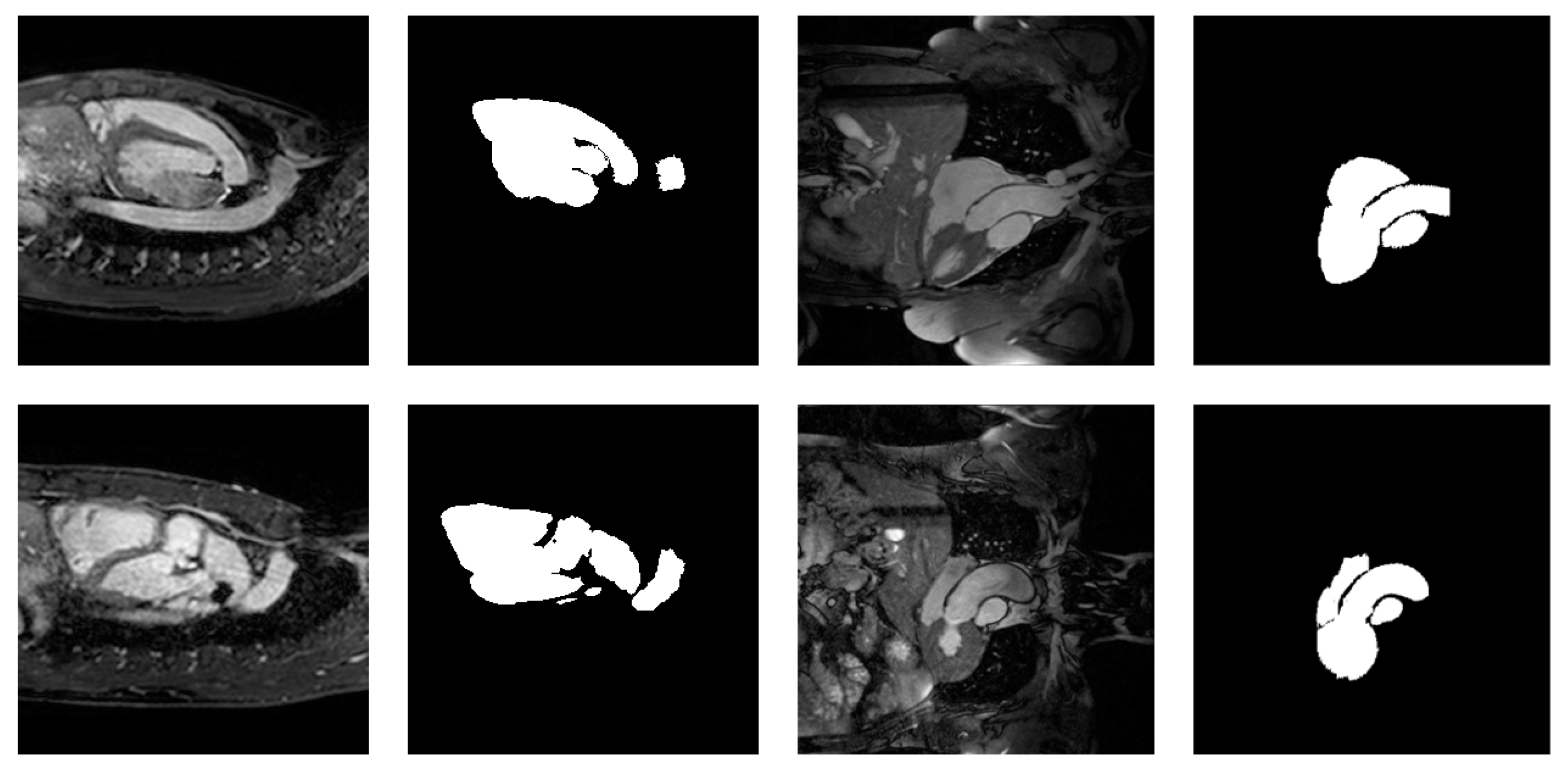
2.1. MRI Whole-Heart Segmentation

The task of MRI whole-heart segmentation (WHS) refers to the outlining of different heart structures from cardiac MRI scans. Recently, the task has received much attention, due, in part, to several open grand challenges and datasets [21,22], which have promoted the development of comparable solutions to the WHS task [23].

The spectrum of the best-performing WHS solution shows a polarization between deep learning-based [24,25] and multi-atlas-based approaches [26,27]. These two sets of approaches are representative of the data-based and bespoke solutions’ dichotomy discussed in Section 1.

Our approach is most similar to a third, less powerful class of approaches, one in which solutions are fully unsupervised; they do not rely on annotated data. Recent work in this direction leverages a more diverse set of methods, such as GANs [28], probabilistic modeling [29], dictionary learning [30], and optical flow [31]. A shared feature of all these approaches is their relatively low cost of transfer to different medical imaging tasks, since they do not rely on annotated data or complex modeling with stringent assumptions.

2.2. Cellular Automata and GrowCut

Cellular automata (CAs) [32] are computational models able to model complex behavior; CAs employ multiple locally-interacting discrete elementary units, called cells, usually arranged in a grid. CAs have been successfully applied to a wide range of problems, such as traffic modeling [33], structural design [34], edge detection [35], and image segmentation.

A popular approach to CA-based image segmentation is the GrowCut algorithm introduced in [19]. GrowCut is an interactive image segmentation algorithm, meaning that it requires the user to select a set of seed pixels that mark the segments of the image (e.g., background, object of interest).

GrowCut [19] maps the pixels of the image to a grid of cells, some of which are pre-labeled through the seeding mechanism (the user provides the labels). The state of a cell p in the CA is defined as a triplet $(l_p,{\sigma }_p,C_p)$ where $l_p$ is the label of the cell, ${\sigma }_p$ is its strength, and $C_p$ is a feature value:

• The labels encode the desired segments of the image. At any point, the set of cells having a specific label determines the corresponding pixels of the specific segment.
• The strength of a cell is a value bounded to $[0,1]$, which weakly corresponds to the confidence of the algorithm in the label of the cell. Strengths are used by the algorithm to make decisions relating to label propagation between neighboring cells. Usually, the cells corresponding to the seeds have a maximum strength of one.
• The feature value is an image feature associated with the cell. Most commonly, this is the grey intensity or RGB vector of the pixel corresponding to the cell.

GrowCut evolves at each step by locally propagating labels based on the feature similarity between neighboring cells, until a stable configuration is reached. More specifically, at each time step, a cell p will receive the label ${\lambda }_q$ from a neighbor cell q if the strength ${\sigma }_q$ of cell q combined with the cells’ similarity is larger than ${\sigma }_p$, the strength of p. This is formalized in the GrowCut label propagation condition: ${\sigma }_p<g\left(∥C_p-C_q∥\right)·{\sigma }_q$. This similarity between the cells’ features is given by the function $g(·)$, bounded on $[0,1]$, which transforms the feature difference $∥C_p-C_q∥$ into a similarity. Algorithm 1 details the GrowCut dynamics.

Algorithm 1 Classical GrowCut algorithm applied on an input image I.

1: procedureGrowCut(I) 2:     for $p\in I$ do 3:          ${\sigma }_{defense}\leftarrow {\sigma }_p^t$ 4:          $l_{winning}\leftarrow l_p^t$ 5:          for $q\in N\left(p\right)$ do 6:               if q is in image bound then 7:                   ${\sigma }_{attack}\leftarrow {\sigma }_q^t·g\left(∥C_p-C_q∥\right)$ 8:                   if ${\sigma }_{attack}>{\sigma }_{defense}$ then 9:                        ${\sigma }_{defense}\leftarrow {\sigma }_{attack}$ 10:                       $l_{winning}\leftarrow l_q^t$ 11:         ${\sigma }_p^{t+1}\leftarrow {\sigma }_{defense}$ 12:         $l_p^{t+1}\leftarrow l_{winning}$

2.3. Band-Based GrowCut

For GrowCut, the most popular neighborhood systems used are Moore and von Neumann of radius one [19]. In [36], the authors proposed an extension to GrowCut that augments the local neighborhoods by the addition of remote neighbor bands. For the ease of reference, we call this extension band-based GrowCut (BBG). Thus, in BBG, a cell interacts with both adjacent cells and non-adjacent ones, at a specific distance from the cell. By interacting with remote neighbors, BBG is able to include more global information in the label propagation process.

BBG is parametrized by the extent of the remote neighbor bands, $(a-b)$, which specifies that remote neighbors lie at a distance between a and b to the cell; different distance metrics give different topologies, e.g., extended Moore corresponds to $l_{\infty }$ and extended von Neumann to $l_1$. Since the number of neighbors in these bands grows as a power law with respect to the remote band extent (with a power coefficient that depends on the grid dimensionality), it is not tractable to consider all neighbors in these bands. Thus, a sampling mechanism is used, where, at each step, for each cell, k neighbors are sampled uniformly from the remote neighborhood. Moreover, BBG is relatively robust to the choice of k, with $k=5$ being a sensitive choice.

2.4. Unsupervised GrowCut

Unsupervised GrowCut [37] along with its extensions [38,39] are algorithms based on GrowCut that remove the need for user-provided seeds. These algorithms generate seeds randomly and assign a different label to each pixel in the seed. Starting from these seeds, a label propagation mechanism similar to GrowCut is used to label non-seed pixels. Additionally, a region merging mechanism is used to reduce the number of labels; typically, a threshold on neighboring cells’ similarity is used to determine whether the cells’ labels should be merged. A disadvantage of such methods is the difficulty to control the number of resulting labels, which is usually different from the number of labels required by the specific image segmentation task. Hence, unsupervised GrowCut cannot be readily used for higher level tasks such as semantic segmentation or instance segmentation, since it requires a post-processing step that determines the nature (with respect to the task) of each generated region.

3. Seeds for Image Segmentation

GrowCut and its extensions have been successfully used in image segmentation tasks. However, the algorithm relies on a user-specified seed in order to perform well. Generating such seeds automatically is an easier task than segmenting the entire image: we only need to find a relatively small set of pixels that mark the image segments with high precision.

The generated seeds trade off the seed size and seed precision: seed size refers to the number of pixels making up the seed, while seed precision refers to the fraction of these pixels that overlap with the true object of interest (OOI). This trade-off is necessary, since a seed of maximum size and precision coincides with a perfect segmentation. Moreover, the trade-off is also affected by the specifics of the task, such as inherent variance in the OOIs, the difficulty of modeling OOIs, and the noise profile.

For these reasons, assessing the feasibility of generated seeds entails the exploration of the trade-off’s regimes and GrowCut’s response to them.

3.1. Automatic Seeds

Automatically generated seeds have been presented in the literature in both explicit and implicit forms. Notably, in [40], the authors presented an overview of seed selection mechanisms for the seeded region growing algorithm [41,42] in bio-medical applications. Most of the surveyed studies focus on finding a single seed point in the image, as well as the region growing threshold. All such methods rely on task-specific knowledge that is used in the process of seed selection.

For example, in lesion detection from ultrasound tasks [43,44], seeds are selected by taking into account homogeneity and grey intensity, based on the observation that lesions in ultrasound have a high intensity and are homogeneous. Similar assumptions were used by [45,46] for breast lesion detection in MRI scans.

In [47], the authors presented a method for selecting seed points in MRI scans for organ detection. The method relies on extracting a set of features (Haralick, semi-variogram, Gabor) and using these to construct a scoring function for each pixel in the image. Then, the pixel that minimizes the scoring function is selected as a seed point. To the best of our knowledge, this is the only method that we found to solve a similar task to the one we are investigating: cardiac MRI image analysis.

An implicit seed generation strategy is embedded in the Unsupervised GrowCut method [37]. Here, instead of modeling the seeds and generating them based on domain knowledge, the location and label of the seeds are generated randomly, and segmentation proceeds by expanding and merging seed regions.

3.2. Seeds in Controlled Experiments

Another category of seeds is represented by seeds generated from the ground truth segmentation. This type of seed is an excellent tool for analyzing the properties of seeded algorithms, while avoiding the bias and variance introduced by manual segmentations. An example of such seeds is the vertical seeding mechanism used in [36], which deterministically generates seeds in the shape of 1 px wide vertical lines.

In our experiments, we used such a type of seed in order to control seed properties, while avoiding biases introduced by manual segmentation. Concretely, this is a random walk-based (foreground) seed generation process that allows us to control the seed size n and seed precision $\pi$. The process of generating such seeds starts by randomly choosing a pixel on the border of the OOI (We also filter the border pixels by ensuring that the proportion of foreground pixels in a 7 × 7 vicinity is between 0.3 and 0.7. This was done in order to avoid situations where there are not enough foreground/background pixels for the random walk). From this initial pixel, two random walks are performed on the true segmentation mask—one representing the pixels agreeing with the ground truth and one set of false positive pixels:

• A random walk of size $n\times \pi$ that evolves along the foreground.
• A random walk of size $n\times (1-\pi )$ that evolves along the background.

Whenever a random walk is unable to advance, the algorithm backtracks to a previous state and continues the walk from there.

4. Seed Generation for MRI Whole-Heart Segmentation

In order to reify the feasibility of automatically generated seeds, we propose a method for whole-heart segmentation of MRI images, based on generated seeds. The method is based on standard edge detection and local thresholding methods, and it is grounded on observations about the structure of the task.

4.1. Task Invariants

In order to simplify the task of generating seeds, we introduce structure in the task in the form of two invariants related to the OOI:

• OOI centeredness: the object of interest (the heart) is positioned near the center of the image, having similar scale across images.
• OOI local brightness: OOI is represented by higher gray intensity in its immediately local area.

Figure 1 exemplifies these invariants with sample images from the MMWHS dataset [21].

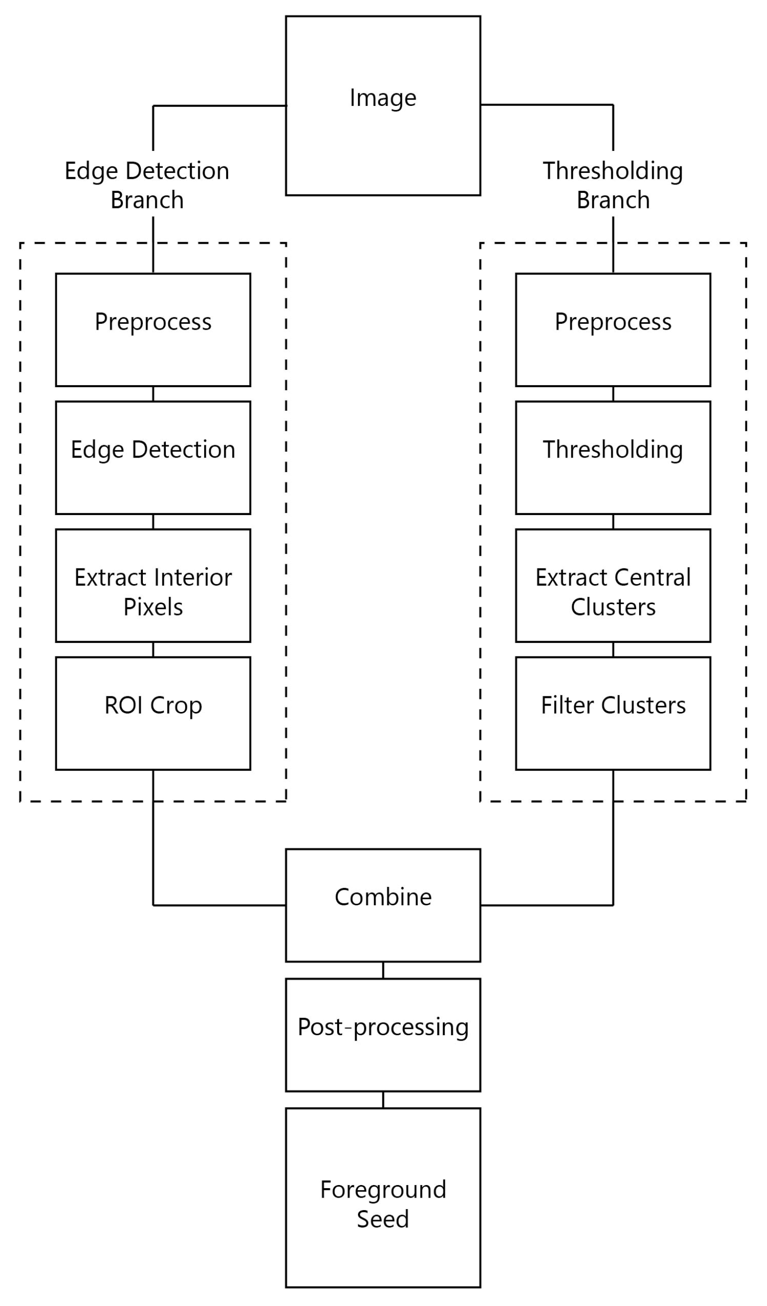
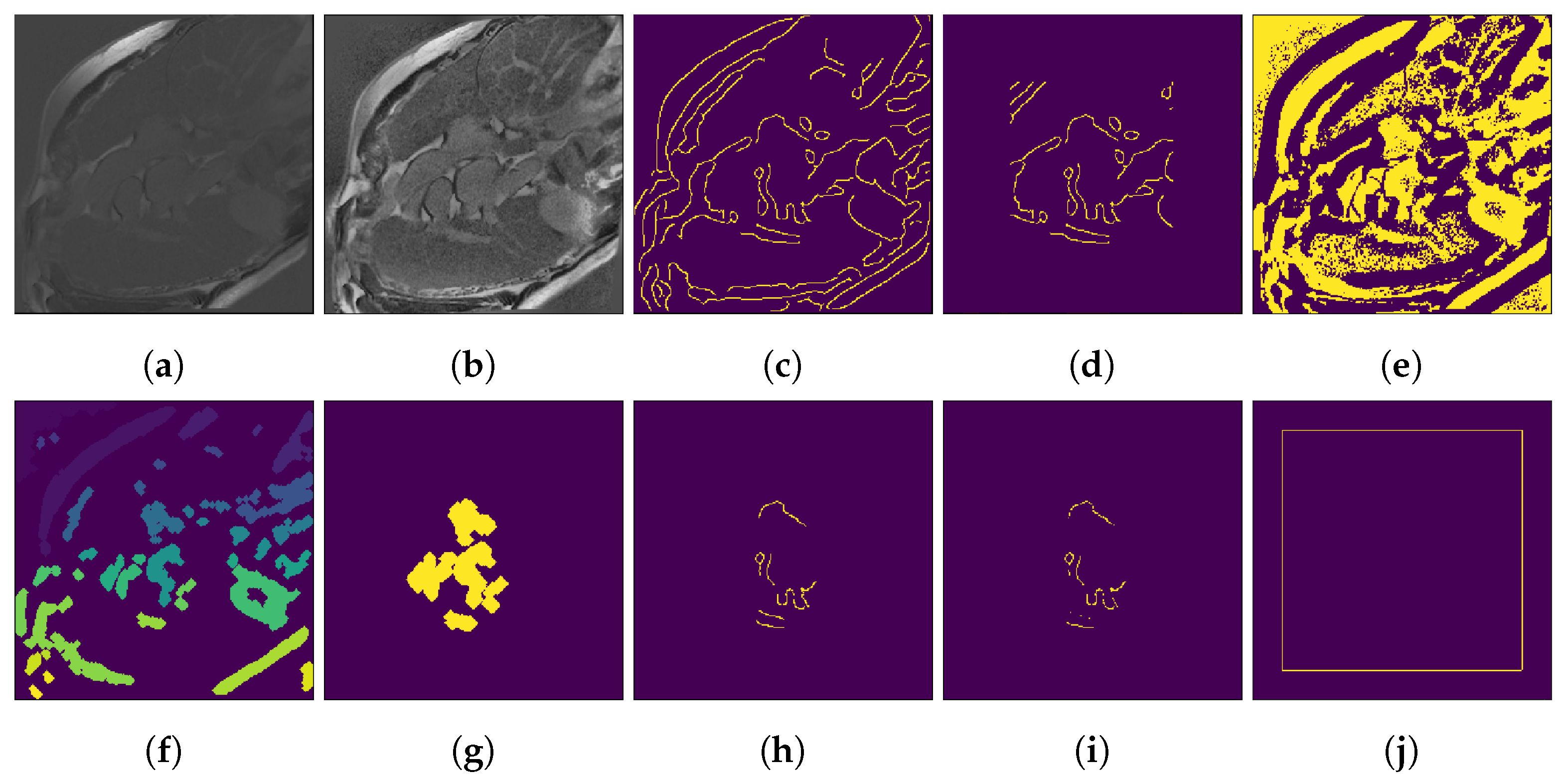
4.2. Method Pipeline

The centeredness invariant gives us a method to generate the bounds of a region that contains the heart. Moreover, defining such a region provides us with a trivial seed for the background of the image. Specifically, for the background seed of an image, we use lines of pixels that are a fixed distance away from the border of the image.

For the foreground seed, we use an image processing pipeline to generate a small set of pixels marking the OOI (illustrated in Figure 2).

The pipeline is made of two branches: edge detection and thresholding. Each of these branches generates a seed proposal based on the particular method. The two proposals are combined to generate only one set of seed points that is further post-processed to increase its precision.

The edge detection branch is composed of four steps. First, the image is preprocessed such that it is more suitable to edge detection. Second, an edge detection procedure is carried out. Since edges describe the contour of object, we generate pixels that are inside the object by using these edges. These edges are an indicator of the OOI extent, especially in the central region of the image. For this reason, in the last step, we crop the edge detector output to a rectangular region of interest (ROI).

The thresholding branch is similar to the edge detection one. We first preprocess the image and then feed it to a thresholding algorithm. Using this thresholding, we aim to find large connected components that have a high chance of belonging to the OOI. To this end, we split the thresholding output into connected components and extract the components closest to the most central component. Finally, we apply a filtering step on these components. The details and parameters of the pipeline are presented in the next section.

4.3. Method Details

For the foreground seed pipeline, we used the following specialization of the steps illustrated in Figure 2. An example of the output of these steps is presented in Figure 3.

In the edge detection branch, images are first preprocessed by a contrast-limited adaptive histogram equalization (CLAHE) [48] step that prepares the image for edge detection (Figure 3b). After this, the Canny edge detector is used to extract edges from the image (Figure 3c). To generate pixels inside the object, we move all edges towards the center of the image by 1 px. Further, we crop the edge detector output to an ROI that sits 70 px away from the image border (Figure 3d); this is, a value for which the heart is included in the ROI for all resolutions in the datasets. It is worth noting that the ROI parameter trades off seed precision and recall. Moreover, this is the only parameter fixed in favor of recall; a larger ROI implies a larger universe of possible seed pixels and, thus, a possible increase in recall.

In the thresholding branch, the same CLAHE preprocessing is used. For thresholding, we run a local Otsu thresholding (Figure 3e) and generate the connected components. We filter out those with an area under 50 px (Figure 3f), since these are mostly noise; a higher area threshold promotes seed precision while risking filtering out important heart structures. We then extract the components closest to the most central one and apply a dilation step of 1 px (Figure 3g). This last step ensures that when combining the result with the output of the edge detection branch, we are not discarding edge pixels. The number of dilation steps can be interpreted as a dual of the distance the seeds are moved towards the center in the edge detection branch.

Since we aim to obtain a relatively small, high-precision seed, we combine the two seed proposals by intersecting them (Figure 3h). Finally, we post-process the seed by removing the top 20% lowest-intensity pixels (Figure 3i), giving the final foreground seed. We set the 20% parameter conservatively, in order to have a high probability of removing any low-intensity outliers.

In the case of the background seed, we used 1 px wide lines sitting at 25 px from the border of the image. This background seed is illustrated in Figure 3j.

4.4. Computational Complexity

For seed generation, the complexity of the proposed method follows from the complexities of the pipeline components. Thus, the seed generation pipeline has a linear complexity with respect to the number of pixels in the input image.

Table 1. Computational complexities of the seed generation pipeline as a function of n, the number of pixels in the input image. CLAHE, contrast-limited adaptive histogram equalization.

Branch	Stage	Complexity
Edge	CLAHE	$\mathcal{O}\left(n\right)$
Edge	Canny	$\mathcal{O}\left(n\right)$
Edge	Move + crop	$\mathcal{O}\left(n\right)$
Thresholding	Otsu	$\mathcal{O}\left(n\right)$
Thresholding	Connected components	$\mathcal{O}\left(n\right)$
Thresholding	Filter + extract central component	$\mathcal{O}\left(n\right)$
Thresholding	Dilation	$\mathcal{O}\left(n\right)$
Post-process	Intersection	$\mathcal{O}\left(n\right)$
Post-process	Intensity filter	$\mathcal{O}\left(n\right)$

details the complexities of the different pipeline stages. Finally, the segmentation step has a complexity of $\mathcal{O}\left(nk\right|\mathcal{N}\left|\right|C\left|\right)$, where:

• n is the number of pixels in the input image
• k is the number of iterations for which the algorithm is run
• $\left|\mathcal{N}\right|$ is the cardinality of the neighborhood system used; e.g., this is eight for GrowCut and 13 for BGC (five extra random remote neighbors)
• $\left|C\right|$ is the dimension of the image feature representation. This is one in our case (grayscale images), but can be larger if other feature spaces are used (e.g., texture descriptors or deep learning-based representations).

5. Experiments and Results

In order to evaluate the proposed seed generation method, we performed the following analyses:

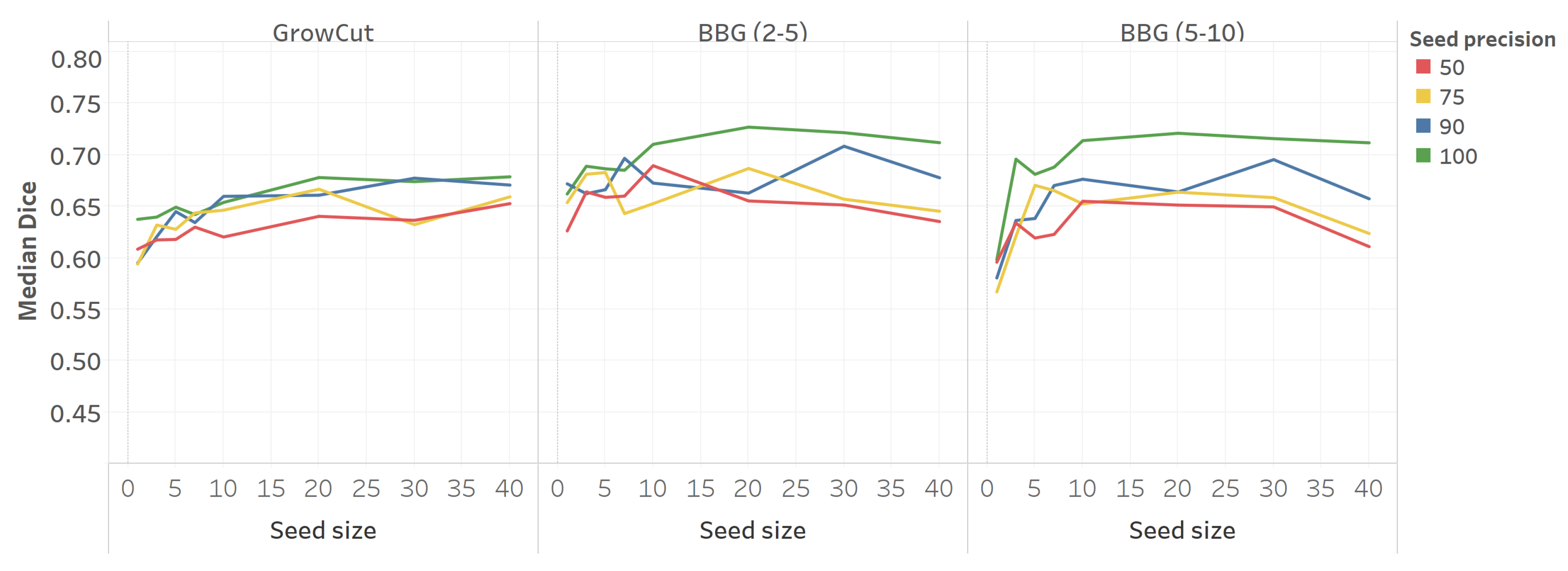
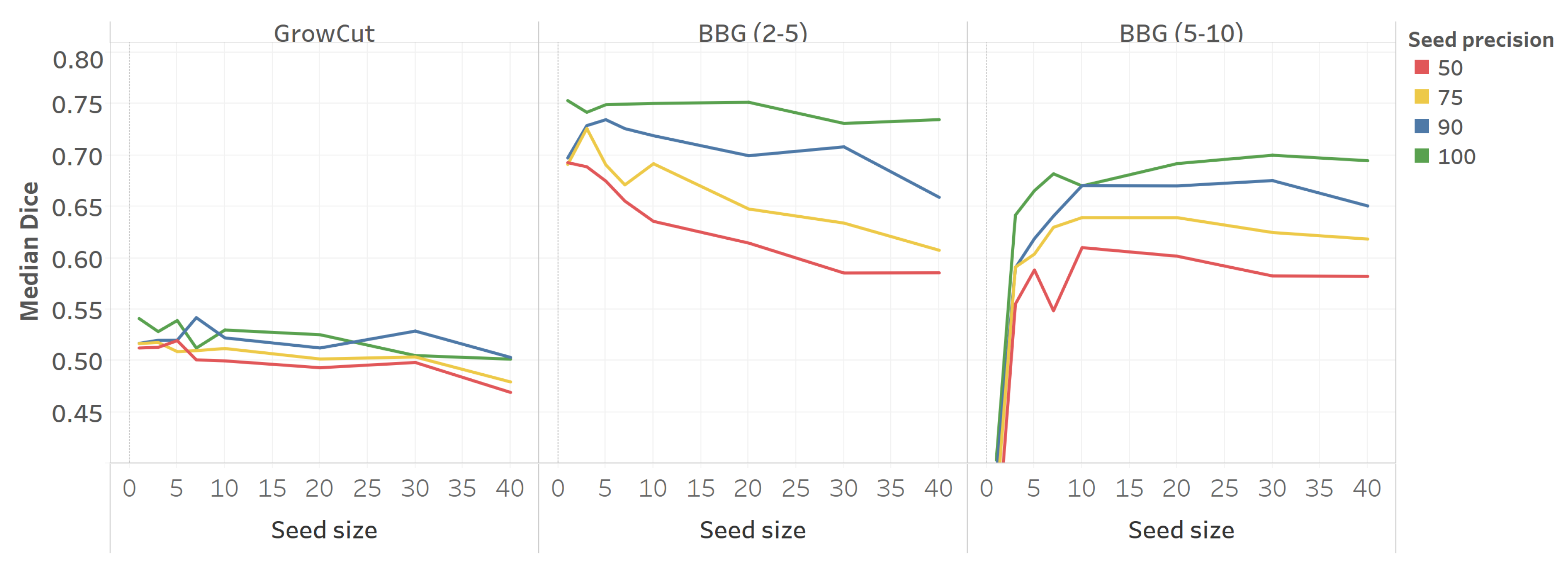
• Effects of seed size and seed precision on the segmentation performance (Section 5.4).
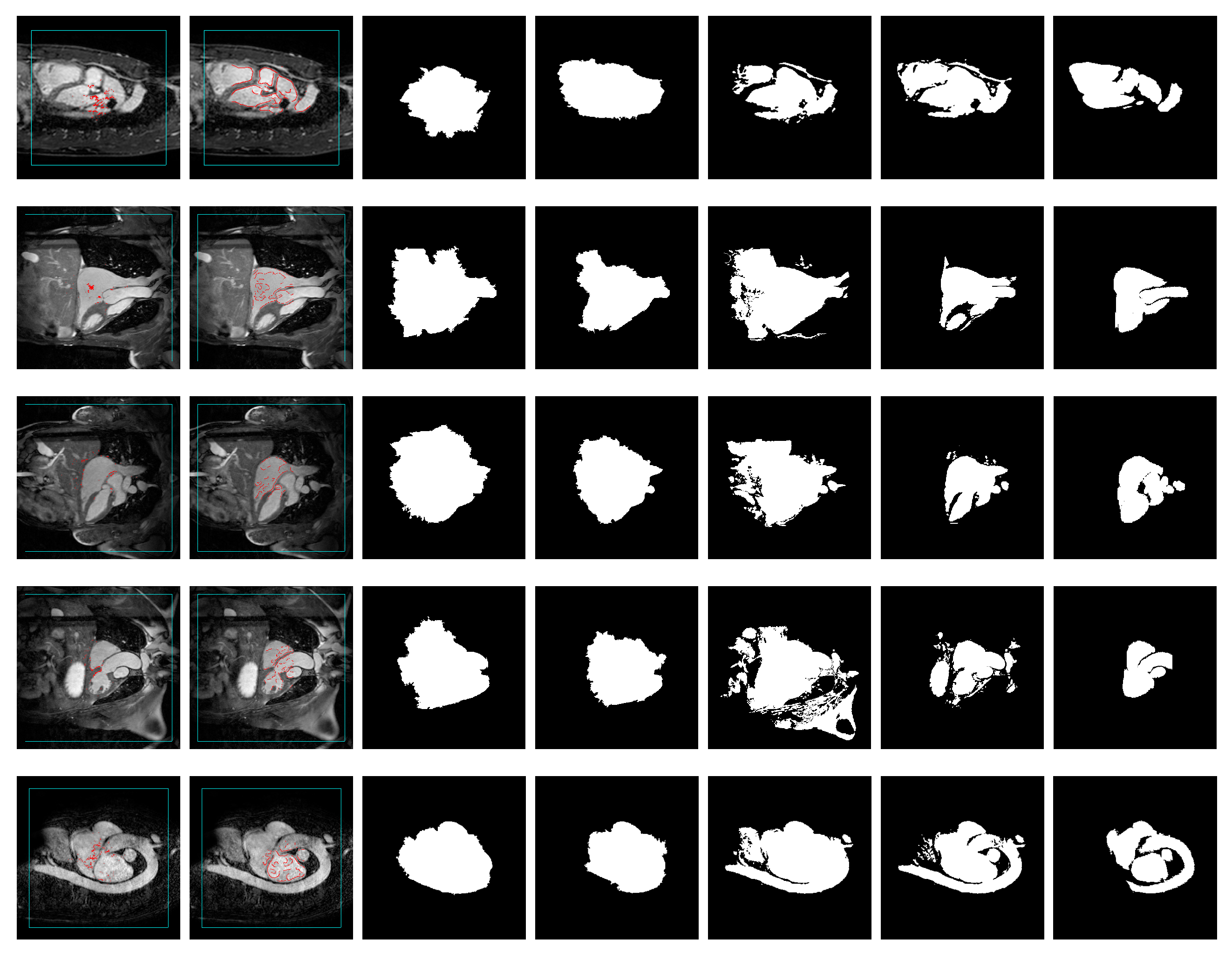
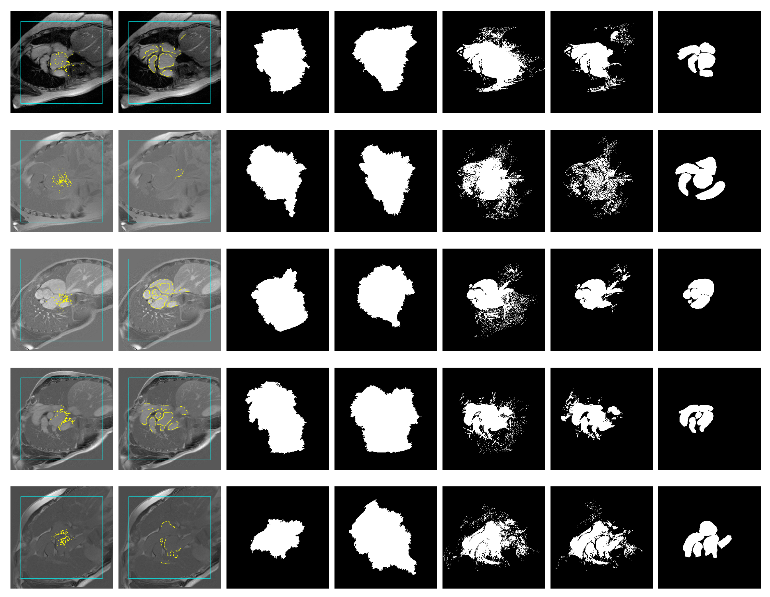
• Evaluation of the proposed seed generation method, contrasted with a similar technique from the literature and unsupervised GrowCut (Section 5.5).

5.1. Data

We ran experiments on the Multi-Modality Whole Heart Segmentation (MMWHS) dataset [21], a dataset of 2.5D (stacks of 2D images) MRI and CT scans of the human heart ranging in dimension from 256 px × 256 px to 512 px × 512 px. We used 20 MRI scans of this dataset, along with ground truth volumes that segment the heart chambers from the rest of the scan. For each stack of slices, we only used the most representative slice (i.e., the one with the largest heart area).

We also used a dataset of 2.5D cardiac MRI scans from our concurrent study on atrial fibrillation (imATFIB—NCT03584126). The dataset consists of 20 stacks of slices (from which we selected the most representative slice) of dimension 256 px × 256 px. The ground truth was prepared by a team of two radiologists: one radiologist manually segmented the heart structures, while a second, more experienced, radiologist validated the manual segmentations.

In order to simplify the interpretation of the results, for each dataset, we solved the problem of segmenting the entire heart region without differentiating between the different structures of the heart.

5.2. Algorithm Parameters

We used two flavors of the GrowCut algorithm for our experiments: classical GrowCut [19] and band-based GrowCut (BBG) [36]. For both algorithms, we used Moore neighborhoods with radius one and, in the case of BBG, remote bands spanning (2,5) and (5,10) pixels with five neighbors sampled at each step (as used in [36]). In all experiments, we set an upper limit of iterations to 2000, where, if convergence is not reached, execution is stopped, and the intermediate labeling is used as the final one.

5.3. Seeds

For our feasibility analysis, we used a random walk-based seed generation process (presented in Section 3.2). This method allows us to control the seed size n (total number of seed pixels) and seed precision $\pi$ (fraction of seed pixels that overlap with the ground truth). All foreground seeds generated in our analyses were complemented by a background seed represented by a frame near the image border. Using such a fixed background seed ensured that we did not introduce additional variance in the segmentation results.

5.4. Seed Generation Feasibility

To assess the feasibility of automatically generating seeds, we explored the seed size and seed precision trade-off on the MMWHS and imATFIB datasets. To this end, we generated seeds with size $n\in \{1,3,5,7,10,20,30,40\}$ and precision $\pi \in \{0.50,0.75,0.90,1.00\}$. Moreover, to account for the variance introduced by the random walk process, we generated 10 sets of seeds for each size/precision configuration. This setup aims to answer the question: Can small, low-precision seeds behave similarly, from the point of view of segmentation performance, to larger, higher precision seeds? In other words, we are interested in assessing whether segmentation performance scales significantly with seed size and seed precision.

Figure 4 shows the segmentation performance related to different configurations of seed size and seed precision.

For all three GrowCut configurations, there is a seed size threshold after which the average Dice value stabilizes. Thus, for a seed size greater than 10, neither GrowCut nor BBG (2–5) show a significant improvement in the Dice value. Similarly, for BBG (5–10), no significant improvement in performance is observed for seed sizes greater than 20.

Seed precision influences the performance of the algorithm, most notably in large seed size regimes for BBG. Although seed precision predicts the relative ordering with respect to segmentation performance, the largest absolute difference in the average Dice value is still smaller than 0.1.

For the completeness of the analysis, we also computed the effect size, using the ${\omega }^2$ statistic [49], of the two factors (seed size and precision) on the segmentation performance. We did this separately for each algorithm configuration. Moreover, we also filtered the data to seed sizes greater than 10 to restrict our analysis to more stable seeds. For this, we first performed a two-way ANOVA analysis and computed the p-value of the interaction terms, which showed the lack of a significant interaction between the two factors (p-values 0.65, 0.50, 0.32 for GrowCut, BBG (2–5), BBG (5–10), respectively).

The obtained ${\omega }^2$ statistics are shown in

Table 2. ${\omega }^2$ statistic (effect size) for the seed size and precision factors (MMWHS dataset).

	GrowCut	BBG (2–5)	BBG (5–10)
Seed size ${\omega }^2$	0.0002	0.0002	0.0018
Precision ${\omega }^2$	0.0040	0.0149	0.0104

. According to [50], these are considered to be either small (${\omega }^2\in (0.01,0.06]$) or very small (${\omega }^2<0.01$) effect sizes.

We obtained similar results for the imATFIB dataset. Figure 5 shows the relation between segmentation performance, seed size, and seed precision. While the general conclusions are similar, the imATFIB dataset shows more variance in the different seed precision curves.

Table 3. ${\omega }^2$ statistic (effect size) for the seed size and precision factors (imATFIB dataset).

	GrowCut	BBG (2–5)	BBG (5–10)
Seed size ${\omega }^2$	0.0026	0.0142	0.0919
Precision ${\omega }^2$	0.0019	0.0339	0.0182

shows the ${\omega }^2$ values for the imATFIB dataset; the same conclusions apply to this dataset, with an exception for the seed size factor in the case of BBG (5–10). While this factor shows a non-small effect size, we can see in the figure that the median performance shows a decreasing trend towards higher seed sizes, which is in consonance with the rest of the conclusions.

These results suggest that, for seeds that are reasonably large (above ten pixels in our case), small seed size and precision do not have a significant effect on the segmentation performance. This suggests that the GrowCut suite of algorithms is robust to seed noise, making automatic seed generation feasible.

5.5. Evaluation of the Proposed Method

5.5.1. Feature- and Texture-Based Seeding

In [47], a method of automatically-seeded segmentation was proposed for organ detection in MRI scans. For conciseness, we further refer to this method as feature- and texture-based seeding (FTS). FTS’s setup differs from ours in two ways. Firstly, the method is designed for a different seeded segmentation algorithm, seeded region growing (SRG) [41], which is based on region growing until a threshold condition is met. Thus, SRG does not require a background seed; moreover, it is usually used with just one foreground seed pixel, centered in the object of interest. Secondly, SRG assumes that the image is cropped to an ROI whose center aligns with that of the organ to be segmented.

In order to apply this method to our scenario, we perform slight modifications that adapt FTS to our tasks:

• Multiple seed pixels: We adapted the method to select multiple pixels, rather than just one. This was achieved by selecting the top pixels sorted by the cost value used by the original method. In our experiments, we used 300 seed pixels.
• Background seed: Since the method does not produce any background seed, we used the same generator as for our method (i.e., a 1 px square sitting 25 px from the border of the image).
• Different cost function weights: FTS works by computing a cost function and selecting the top pixel in the ROI according to it. The cost function has three components: spatial centrality (spatial distance to the center of the ROI), feature distance (distance in the feature space from the ROI mean feature vector), neighborhood homogeneity (sum of feature distances from the neighbors of a pixel). In our experiments, if we balanced all these components to have the same weight and scale, we obtained seeds that were centered around the center of the ROI, since the spatial centrality component dominated the entire cost function. In order to escape this, we explored different weights for the cost components and fixed them to 0.2 (spatial centrality), 0.7 (feature distance), and 0.1 (neighborhood homogeneity).

Out of the four feature representations proposed in the FTS paper (Haralick, Gabor, 2D semi-variogram, and 3D semi-variogram), we found that the Haralick representation offered the best result.

5.5.2. Unsupervised GrowCut

Unsupervised GrowCut (UGC) outputs a segmentation that contains an uncontrolled number of labels. In order to assess UGC’s performance on the MMWHS and imATFIB segmentation tasks, we need to either force UGC to output the desired number of labels (i.e., background and foreground) or relabel the resulting segments with the target labels. Similar to the evaluation used in the original UGC paper [37], for each image in the dataset, we varied the merge threshold parameter and selected the one that yielded the desired number of labels. For a target number of two labels, this strategy provided poor results: 0.17 and 0.14 Dice scores on the MMWHS and imATFIB datasets, respectively.

Note that we chose to vary the threshold parameter, rather than the number of seed pixels (as in the original paper’s experiment design), since this is a parameter that is much more robust to the random seed initialization of UGC. Moreover, the noise introduced by the random seed is amplified when targeting a small number of labels, since this is achieved for a very small number of seed pixels. This is further complicated by the resolution of the images (between $256\times 256$ and $512\times 512$ as opposed to $64\times 64$ in the UGC paper, where the strategy was used).

To improve the UGC baseline, we experimented with relabeling the segments output by UGC, rather than forcing the number of segments. In order to find the UGC parameters, we fixed the threshold to 0.95, as proposed in the original paper, and searched over the number of initial seed pixels for each image. Note that, in this scenario, it is feasible to use the number of seed pixels as a search variable, since we are not constraining the number of target segments. To account for the various image sizes, we performed our search over seed density $\rho$: the ratio between the number of seed pixels and the number of total pixels in the image.Our search was performed over 17 values for $\rho$ that increased in a quadratic manner (We used the following values: $2.44\times {10}^{-5}$, $1.22\times {10}^{-4}$, $2.44\times {10}^{-4}$, $7.32\times {10}^{-4}$, $1.22\times {10}^{-3}$, $2.44\times {10}^{-3}$, $4.88\times {10}^{-3}$, $7.32\times {10}^{-3}$, $9.77\times {10}^{-3}$, $1.34\times {10}^{-2}$, $1.83\times {10}^{-2}$, $2.44\times {10}^{-2}$, $3.17\times {10}^{-2}$, $4.03\times {10}^{-2}$, $5.00\times {10}^{-2}$, $6.10\times {10}^{-2}$, $7.32\times {10}^{-2}$. These were obtained by translating from an absolute number of seed pixels for $64\times 64$ px images, as used in the original paper. Thus, the $\rho$ values used correspond to $0.1,0.5,1,3,5,10,20,30,40,55,75,100,130,165,205,250,300$ seed pixels in the $64\times 64$ images).

For each image and value of the seed density, we performed the segmentation and recorded the total within cluster sum of squares (TWCSS) [51]: this measures, for all segments of the image, the sum of squared differences between the pixel intensities and the mean intensity. More formally, TWCSS can be defined as:

$$TWCSS=\sum _{S\in \mathcal{S}}\sum _{p\in S}{(I\left(p\right)-{\mu }_S)}^2$$

where $\mathcal{S}$ is the set of segments output by UGC, p iterates over pixels belonging to a segment S, $I\left(p\right)$ is the intensity of pixel p in the image, and ${\mu }_S$ is the mean intensity of all pixels belonging to segment S. Finally, for each image, we manually chose the seed density value using the elbow method [51] of optimizing the number of clusters.

In order to relabel the segments obtained by UGC, we assigned the background label to the segments that included the four corners of the image and labeled as foreground all the other segments. We experimented with labeling the unlabeled pixels as the background and with a combined strategy that assigns the background label to both the corner segments and the unlabeled pixels, also. None of these approaches provided better results, though.

Using this parameter selection and relabeling approach, we obtained a median Dice coefficient of 0.36 and 0.16 for the MMWHS and imATFIB datasets, respectively. Similar results (0.40 and 0.14 median Dice value for MMWHS and imATFIB, respectively) were obtained if we selected the seed density based on the number of labels in the segmentation, rather than TWCSS.

5.5.3. Evaluation

Table 4. Median Dice coefficient values obtained using our method, FTS, and unsupervised GrowCut (UGC).

	Contour Seed (Ours)			FTS (Haralick)			UGC
	GrowCut	BBG (2–5)	BBG (5–10)	GrowCut	BBG (2–5)	BBG (5–10)
MMWHS	0.65	0.76	0.76	0.58	0.61	0.61	0.40
imATFIB	0.42	0.70	0.71	0.51	0.67	0.64	0.14

shows the median results obtained using our proposed seeding method, FTS, and UGC;

Table 5. Ninety-five percent confidence interval of Dice coefficient values obtained using our method, FTS, and UGC.

	Contour Seed (Ours)			FTS (Haralick)			UGC
	GrowCut	BBG (2–5)	BBG (5–10)	GrowCut	BBG (2–5)	BBG (5–10)
MMWHS	[0.62, 0.72]	[0.70, 0.79]	[0.69, 0.78]	[0.54, 0.65]	[0.58, 0.68]	[0.56, 0.69]	[0.46, 0.45]
imATFIB	[0.37, 0.45]	[0.67, 0.73]	[0.67, 0.73]	[0.42, 0.56]	[0.58, 0.70]	[0.54, 0.67]	[0.09, 0.20]

complements the results with 95% confidence intervals. Figure 6 and Figure 7 show examples of the segmentation output for the MMWHS and imATFIB datasets, respectively.

The results suggest that our proposed method and FTS outperform UGC. Moreover, none of the GrowCut-based approaches has the downside of requiring manual tuning of parameters.

Our proposed method performs best in the BBG cases, while, in the GrowCut cases, the best performing method is a function of the dataset. These results further reinforce the feasibility of seed generation and show that good segmentation results can be obtained with seed-level modeling based on simple observations about the task.

5.6. Discussion

Our method shows several desirable properties, such as an unsupervised character and robustness to seed precision. These properties, though, can be seen as the result of trading off segmentation performance. As illustrated in

Table 6. Dice coefficients obtained by supervised techniques compared to our proposed method as evaluated within the MMWHS grand challenge [23].

Ours	Non-Local Fusion [27]	Local Probabilistic Atlases [26]	Anatomic Label Configurations [24]
0.76	0.87	0.82	0.86

, deep learning and multi-atlas-based approaches outperform our solution. Nevertheless, our method shows similar performance to recent unsupervised whole-heart segmentation methods [28,29,30,31], both qualitatively and quantitatively (Reference [28] reports a Dice coefficient of 0.66, while our BBG (5–10) configuration achieves a Dice coefficient of 0.76).

6. Conclusions

In this paper, we experimentally showed the feasibility of automating the seed generation process for the GrowCut algorithm on the task of MRI whole-heart segmentation. This entails that using seeded image segmentation algorithms, such as GrowCut coupled with a domain-specific seed generation method, can greatly simplify the task of modeling solutions for image segmentation.

We further reinforced this by proposing a method of generating such seeds using minimal modeling and domain knowledge. Concretely, we propagate structure in the MRI images specific to the task and design a method to generate input seeds.

We demonstrate the method on two cardiac MRI datasets and contrast it with unsupervised GrowCut and a similar seed generation method proposed in the literature [47].

In the future, we plan to:

• Investigate the interaction between different seed properties and segmentation performance, both in supervised and imperfect precision regimes.
• Design more sophisticated computer vision methods for a better control over the proposed seed properties.

The method presented in this paper could be used in an automated image processing pipeline in a computer aided diagnosis system. Such automatic algorithms will augment human decision making and, in the future, will provide a decision support for radiologists, increasing the quantitative diagnostic.

References

1. Masood, S.; Sharif, M.; Masood, A.; Yasmin, M.; Raza, M. A survey on medical image segmentation. Curr. Med. Imaging Rev. 2015, 11, 3–14. [Google Scholar] [CrossRef]
2. Zaitoun, N.M.; Aqel, M.J. Survey on image segmentation techniques. Procedia Comput. Sci. 2015, 65, 797–806. [Google Scholar] [CrossRef] [Green Version]
3. Hosny, A.; Parmar, C.; Quackenbush, J.; Schwartz, L.H.; Aerts, H.J. Artificial intelligence in radiology. Nat. Rev. Cancer 2018, 18, 500. [Google Scholar] [CrossRef] [PubMed]
4. Wang, S.; Summers, R.M. Machine learning and radiology. Med. Image Anal. 2012, 16, 933–951. [Google Scholar] [CrossRef] [PubMed] [Green Version]
5. Giger, M.L. Machine learning in medical imaging. J. Am. Coll. Radiol. 2018, 15, 512–520. [Google Scholar] [CrossRef] [PubMed]
6. Santos, M.K.; Ferreira Júnior, J.R.; Wada, D.T.; Tenório, A.P.M.; Barbosa, M.H.N.; Marques, P.M.d.A. Artificial intelligence, machine learning, computer-aided diagnosis, and radiomics: Advances in imaging towards to precision medicine. Radiol. Bras. 2019, 52, 387–396. [Google Scholar] [CrossRef] [Green Version]
7. Chan, S.; Siegel, E.L. Will machine learning end the viability of radiology as a thriving medical specialty? Br. J. Radiol. 2019, 92, 20180416. [Google Scholar] [CrossRef]
8. Fritz, S.; See, L.; Perger, C.; McCallum, I.; Schill, C.; Schepaschenko, D.; Duerauer, M.; Karner, M.; Dresel, C.; Laso-Bayas, J.C.; et al. A global dataset of crowdsourced land cover and land use reference data. Sci. Data 2017, 4, 170075. [Google Scholar] [CrossRef] [Green Version]
9. Helber, P.; Bischke, B.; Dengel, A.; Borth, D. Eurosat: A novel dataset and deep learning benchmark for land use and land cover classification. IEEE J. Sel. Top. Appl. Earth Obs. Remote Sens. 2019, 12, 2217–2226. [Google Scholar] [CrossRef] [Green Version]
10. Spera, E.; Furnari, A.; Battiato, S.; Farinella, G.M. EgoCart: A Benchmark Dataset for Large-Scale Indoor Image-Based Localization in Retail Stores. IEEE Trans. Circuits Syst. Video Technol. 2019. [Google Scholar] [CrossRef]
11. Cordts, M.; Omran, M.; Ramos, S.; Rehfeld, T.; Enzweiler, M.; Benenson, R.; Franke, U.; Roth, S.; Schiele, B. The cityscapes dataset for semantic urban scene understanding. In Proceedings of the IEEE Conference on Computer Vision and Pattern Recognition, Las Vegas, NV, USA, 27–30 June 2016; pp. 3213–3223. [Google Scholar]
12. Zhang, C.; Harrison, P.A.; Pan, X.; Li, H.; Sargent, I.; Atkinson, P.M. Scale Sequence Joint Deep Learning (SS-JDL) for land use and land cover classification. Remote Sens. Environ. 2020, 237, 111593. [Google Scholar] [CrossRef]
13. Fu, J.; Liu, J.; Li, Y.; Bao, Y.; Yan, W.; Fang, Z.; Lu, H. Contextual deconvolution network for semantic segmentation. Pattern Recognit. 2020, 101, 107152. [Google Scholar] [CrossRef]
14. Jaware, T.; Khanchandani, K.; Badgujar, R. A novel hybrid atlas-free hierarchical graph-based segmentation of newborn brain MRI using wavelet filter banks. Int. J. Neurosci. 2020, 130, 499–514. [Google Scholar] [CrossRef] [PubMed]
15. Mathew, A.R.; Anto, P.B. Tumor detection and classification of MRI brain image using wavelet transform and SVM. In Proceedings of the 2017 International Conference on Signal Processing and Communication (ICSPC), Tamil Nadu, India, 28–29 July 2017; IEEE: Piscataway, NJ, USA, 2017; pp. 75–78. [Google Scholar]
16. Isensee, F.; Jaeger, P.F.; Full, P.M.; Wolf, I.; Engelhardt, S.; Maier-Hein, K.H. Automatic cardiac disease assessment on cine-MRI via time-series segmentation and domain specific features. In International Workshop on Statistical Atlases and Computational Models of the Heart; Springer: Quebec City, QC, Canada, 2017; pp. 120–129. [Google Scholar]
17. Ranschaert, E.R.; Morozov, S.; Algra, P.R. Artificial Intelligence in Medical Imaging: Opportunities, Applications and Risks; Springer: Berlin/Heidelberg, Germany, 2019. [Google Scholar]
18. Forsyth, D.A.; Ponce, J. Computer Vision: A Modern Approach; Prentice Hall Professional Technical Reference; ACM: New York, NY, USA, 2002. [Google Scholar]
19. Vezhnevets, V.; Konouchine, V. GrowCut—Interactive Multi-Label N-D Image Segmentation By Cellular Automata. In Proceedings of the Graphicon. Russian Academy of Sciences, Novosibirsk Akademgorodok, Russia, 20–24 June 2005; pp. 1–7. [Google Scholar]
20. Zhao, F.; Xie, X. An overview of interactive medical image segmentation. Ann. BMVA 2013, 2013, 1–22. [Google Scholar]
21. Zhuang, X.; Shen, J. Multi-scale patch and multi-modality atlases for whole-heart segmentation of MRI. Med. Image Anal. 2016, 31, 77–87. [Google Scholar] [CrossRef]
22. Bernard, O.; Lalande, A.; Zotti, C.; Cervenansky, F.; Yang, X.; Heng, P.A.; Cetin, I.; Lekadir, K.; Camara, O.; Ballester, M.A.G.; et al. Deep learning techniques for automatic MRI cardiac multi-structures segmentation and diagnosis: Is the problem solved? IEEE Trans. Med. Imaging 2018, 37, 2514–2525. [Google Scholar] [CrossRef]
23. Zhuang, X.; Li, L.; Payer, C.; Štern, D.; Urschler, M.; Heinrich, M.P.; Oster, J.; Wang, C.; Smedby, Ö.; Bian, C.; et al. Evaluation of algorithms for multi-modality whole-heart segmentation: An open-access grand challenge. Med. Image Anal. 2019, 58, 101537. [Google Scholar] [CrossRef]
24. Payer, C.; Štern, D.; Bischof, H.; Urschler, M. Multi-label whole-heart segmentation using CNNs and anatomical label configurations. In International Workshop on Statistical Atlases and Computational Models of the Heart; Springer: Berlin/Heidelberg, Germany, 2017; pp. 190–198. [Google Scholar]
25. Wang, C.; Smedby, Ö. Automatic whole-heart segmentation using deep learning and shape context. In International Workshop on Statistical Atlases and Computational Models of the Heart; Springer: Quebec City, QC, Canada, 2017; pp. 242–249. [Google Scholar]
26. Galisot, G.; Brouard, T.; Ramel, J.Y. Local probabilistic atlases and a posteriori correction for the segmentation of heart images. In International Workshop on Statistical Atlases and Computational Models of the Heart; Springer: Quebec City, QC, Canada, 2017; pp. 207–214. [Google Scholar]
27. Heinrich, M.P.; Oster, J. MRI whole-heart segmentation using discrete nonlinear registration and fast non-local fusion. In International Workshop on Statistical Atlases and Computational Models of the Heart; Springer: Quebec City, QC, Canada, 2017; pp. 233–241. [Google Scholar]
28. Joyce, T.; Chartsias, A.; Tsaftaris, S. Deep Multi-Class Segmentation without Ground-Truth Labels; Medical Imaging with Deep Learning; University of Edinburgh: Edinburgh, UK, 2018. [Google Scholar]
29. Cordero-Grande, L.; Vegas-Sánchez-Ferrero, G.; Casaseca-de-la Higuera, P.; San-Román-Calvar, J.A.; Revilla-Orodea, A.; Martín-Fernández, M.; Alberola-López, C. Unsupervised 4D myocardium segmentation with a Markov Random Field based deformable model. Med. Image Anal. 2011, 15, 283–301. [Google Scholar] [CrossRef]
30. Oksuz, I.; Mukhopadhyay, A.; Dharmakumar, R.; Tsaftaris, S.A. Unsupervised myocardial segmentation for cardiac BOLD. IEEE Trans. Med. Imaging 2017, 36, 2228–2238. [Google Scholar] [CrossRef] [Green Version]
31. Mukhopadhyay, A.; Oksuz, I.; Bevilacqua, M.; Dharmakumar, R.; Tsaftaris, S.A. Unsupervised myocardial segmentation for cardiac MRI. In Proceedings of the International Conference on Medical Image Computing and Computer-Assisted Intervention, Munich, Germany, 5–9 October 2015; Springer: Berlin/Heidelberg, Germany, 2015; pp. 12–20. [Google Scholar]
32. Von Neumann, J. Theory of Self-Reproducing Automata; Burks, A.W., Ed.; University of Illinois Press: Urbana, IL, USA, 1966. [Google Scholar]
33. Gershenson, C.; Rosenblueth, D. Modeling self-organizing traffic lights with elementary cellular automata. Comput. Res. Repos. 2009, 2017. [Google Scholar] [CrossRef]
34. Kita, E.; Toyoda, T. Structural design using cellular automata. Struct. Multidiscip. Optim. 2000, 19, 64–73. [Google Scholar] [CrossRef]
35. Chang, C.L.; Zhang, Y.j.; Gdong, Y.Y. Cellular automata for edge detection of images. In Proceedings of the 2004 International Conference on Machine Learning and Cybernetics (IEEE Cat. No. 04EX826), Shanghai, China, 26–29 August 2004; IEEE: Piscataway, NJ, USA, 2004; Volume 6, pp. 3830–3834. [Google Scholar]
36. Marginean, R.; Andreica, A.; Diosan, L.; Balint, Z. Butterfly effect in chaotic image segmentation. Entropy 2020, in press. [Google Scholar]
37. Ghosh, P.; Antani, S.; Long, L.R.; Thoma, G.R. Unsupervised Grow-Cut: Cellular Automata-Based Medical Image Segmentation. In Proceedings of the 2011 IEEE First International Conference on Healthcare Informatics, Imaging and Systems Biology, San Jose, CA, USA, 26–29 July 2011; IEEE: Piscataway, NJ, USA, 2011; pp. 40–47. [Google Scholar]
38. Marinescu, I.A.; Bálint, Z.; Diosan, L.; Andreica, A. Dynamic autonomous image segmentation based on Grow Cut. In Proceedings of the 26th European Symposium on Artificial Neural Networks (ESANN 2018), Bruges, Belgium, 25–27 April 2018; pp. 67–72. [Google Scholar]
39. Marginean, R.; Andreica, A.; Diosan, L.; Bálint, Z. Autonomous Image Segmentation by Competitive Unsupervised GrowCut. In Proceedings of the 2019 21st International Symposium on Symbolic and Numeric Algorithms for Scientific Computing (SYNASC), Timisoara, Romania, 4–7 September 2019; IEEE: Piscataway, NJ, USA, 2019; pp. 313–319. [Google Scholar]
40. Melouah, A.; Layachi, S. Overview of Automatic seed selection methods for biomedical images segmentation. Int. Arab. J. Inf. Technol. 2018, 15, 499–504. [Google Scholar]
41. Adams, R.; Bischof, L. Seeded region growing. IEEE Trans. Pattern Anal. Mach. Intell. 1994, 16, 641–647. [Google Scholar] [CrossRef] [Green Version]
42. Mehnert, A.; Jackway, P. An improved seeded region growing algorithm. Pattern Recognit. Lett. 1997, 18, 1065–1071. [Google Scholar] [CrossRef]
43. Poonguzhali, S.; Ravindran, G. A complete automatic region growing method for segmentation of masses on ultrasound images. In Proceedings of the 2006 International Conference on Biomedical and Pharmaceutical Engineering, Kuala Lumpur, Malaysia, 11–14 December 2016; IEEE: Piscataway, NJ, USA, 2006; pp. 88–92. [Google Scholar]
44. Shan, J.; Cheng, H.D.; Wang, Y. A novel automatic seed point selection algorithm for breast ultrasound images. In Proceedings of the 2008 19th International Conference on Pattern Recognition, Tampa, FL, USA, 8–11 December 2008; IEEE: Piscataway, NJ, USA, 2008; pp. 1–4. [Google Scholar]
45. Al-Faris, A.Q.; Ngah, U.K.; Isa, N.A.M.; Shuaib, I.L. Breast MRI tumour segmentation using modified automatic seeded region growing based on particle swarm optimization image clustering. In Soft Computing in Industrial Applications; Springer: Berlin/Heidelberg, Germany, 2014; pp. 49–60. [Google Scholar]
46. Al-Faris, A.Q.; Ngah, U.K.; Isa, N.A.M.; Shuaib, I.L. Computer-aided segmentation system for breast MRI tumour using modified automatic seeded region growing (BMRI-MASRG). J. Digit. Imaging 2014, 27, 133–144. [Google Scholar] [CrossRef] [Green Version]
47. Wu, J.; Poehlman, S.; Noseworthy, M.D.; Kamath, M.V. Texture feature based automated seeded region growing in abdominal MRI segmentation. In Proceedings of the 2008 International Conference on BioMedical Engineering and Informatics, Sanya, Hainan, China, 28–30 May 2008; IEEE: Piscataway, NJ, USA, 2008; Volume 2, pp. 263–267. [Google Scholar]
48. Pizer, S.M.; Amburn, E.P.; Austin, J.D.; Cromartie, R.; Geselowitz, A.; Greer, T.; ter Haar Romeny, B.; Zimmerman, J.B.; Zuiderveld, K. Adaptive histogram equalization and its variations. Comput. Vis. Graph. Image Process. 1987, 39, 355–368. [Google Scholar] [CrossRef]
49. Durlak, J.A. How to select, calculate, and interpret effect sizes. J. Pediatr. Psychol. 2009, 34, 917–928. [Google Scholar] [CrossRef] [Green Version]
50. Field, A. Discovering Statistics Using IBM SPSS Statistics; Sage: Thousand Oaks, CA, USA, 2013.
51. Hastie, T.; Tibshirani, R.; Friedman, J. The Elements of Statistical Learning: Data Mining, Inference, and Prediction; Springer Science & Business Media: New York, NY, USA, 2009. [Google Scholar]
Figure 1. Samples from the MMWHS dataset showing four cardiac MRI images along with the manual segmentation of the heart.
Mathematics 08 01511 g001
Figure 2. Pipeline proposed to generate high-precision foreground seeds. Two methods (edge detection and thresholding) are used to generate seed proposals independently. These proposals are further merged and post-processed.
Mathematics 08 01511 g002
Figure 3. Example of automatically generating seeds from an input image. (a) Input image. (b) After adaptive histogram equalization. (c) Canny output. (d) ROI crop of Canny output. (e) Local Otsu output. (f) After applying cluster the area filter on Otsu output. (g) Otsu central components. (h) Canny intersected with central Otsu clusters. (i) After removing top 20% low-intensity pixels (final foreground seed). (j) Trivial background seed.
Mathematics 08 01511 g003
Figure 4. Median Dice value as a function of seed size and seed precision (MMWHS dataset). BBG, band-based GrowCut.
Mathematics 08 01511 g004
Figure 5. Median Dice value as a function of seed size and seed precision (imATFIB dataset).
Mathematics 08 01511 g005
Figure 6. Sample segmentations of MMWHS images. From left to right: image with feature- and texture-based seeding (FTS) (Haralick) seed superimposed (red: foreground, cyan: background), image with contour-based seed superimposed, GrowCut segmentation using FTS (Haralick) seed, GrowCut segmentation using contour-based seed, band-based GrowCut (2–5) segmentation using FTS (Haralick) seed, band-based GrowCut (2–5) segmentation using contour seed, ground truth.
Mathematics 08 01511 g006
Figure 7. Sample segmentations of imATFIB images. From left to right: image with FTS (Haralick) seed superimposed (yellow: foreground, cyan: background), image with contour-based seed superimposed, GrowCut segmentation using FTS (Haralick) seed, GrowCut segmentation using contour-based seed, band-based GrowCut (2–5) segmentation using FTS (Haralick) seed, band-based GrowCut (2–5) segmentation using contour seed, ground truth.
Mathematics 08 01511 g007