Abstract
The progressive iterative approximation (PIA) plays an important role in curve and surface fitting. By using the diagonally compensated reduction of the collocation matrix, we propose the preconditioned progressive iterative approximation (PPIA) to improve the convergence rate of PIA. For most of the normalized totally positive bases, we show that the presented PPIA can accelerate the convergence rate significantly in comparison with the weighted progressive iteration approximation (WPIA) and the progressive iterative approximation with different weights (DWPIA). Furthermore, we propose an inexact variant of the PPIA (IPPIA) to reduce the computational complexity of the PPIA. We introduce the inexact solver of the preconditioning system by employing some state-of-the-art iterative methods. Numerical results show that both the PPIA and the IPPIA converge faster than the WPIA and DWPIA, while the elapsed CPU times of the PPIA and IPPIA are less than those of the WPIA and DWPIA.
1. Introduction
The progressive iterative approximation (PIA) is an important iterative method for fitting a given set of data points. Due to its clear geometric meaning, stable convergence and simple iterative scheme, the PIA has intrigued researchers for decades. In particular, said methodology has achieved great success in geometric design [1,2], data fitting [3,4], reverse engineering [5] and NURBS solid generation [6,7,8]. For more detailed research on this topic, we refer the reader to read a recent survey [9]. However, the PIA converges very slowly, especially when the number of interpolating points increases to some extent. This is because the collocation matrices resulting from some normalized totally positive (NTP) bases are usually ill-conditioned; see [10,11]. Therefore, much more attention was paid to accelerating the convergence rate of PIA; see the weighted progressive iteration approximation (WPIA) (also named modified Richardson method) in [12,13]; the QR-PIA in [11]; the Jacobi-PIA in [14]; the Chebyshev semi-iterative method in [15]; the progressive iterative approximation with different weights (DWPIA) in [16]; the GS-PIA in [17]; the PIA with mutually different weights in [18]; the Schulz iterative method in [19]; and a lot literature therein.
There are other remedy strategies, such as locally interpolating, i.e, interpolating partial points selected from the total given points, which results in the local progressive-iterative approximation format [20], the extended progressive-iterative approximation format [21] and the progressive iterative approximation format for least square fitting [22].
Let be an NTP basis, such as the Bernstein basis [23] or the Said–Ball basis [24]. Given a set of data points in or , we assign a parameter value to the i-th point . For PIA, the initial interpolating curve is given by
and the -th interpolating curve can be generated by
where
Equation (1) can be rewritten as the following form
which generates a sequence of control polygons , for .
Let , , . Then the matrix form of Equations (1) and (2) is
where , , I is the identity matrix and B is the collocation matrix resulting from the basis at , . We note in [23] that the collocation matrix B resulting from any NTP basis is a stochastic totally positive matrix.
If , then the sequence of curves is said to have the PIA property and Equation (2) is referred to as the PIA format. It is shown in [25] that the PIA property holds for any NTP basis.
In fact, the PIA is mathematically equivalent to the Richardson iteration for solving the collocation matrix equation
see [15,26]. Therefore, the state-of-the-art iterative method, the generalized minimal residual (GMRES) method for solving general linear systems of equations, was suggested in [26] for solving (4). It is known that the GMRES method works efficiently when the coefficient matrix B is positive definite. It is true that the GMRES has better convergence behavior than PIA in the same required precision when fitting 19 points on the helix. However, we found that the collocation matrix B resulting from some NTP bases is not always positive definite, even if B is a totally positive matrix. This led us to further study the PIA. Obviously, the convergence of PIA depends on the spectral radius of the iteration matrix . The smaller the spectral radius is, the faster the PIA converges. This motivated us to use the preconditioning techniques to reduce the spectral radius of the iteration matrix . The PIA consists of the interpolatory PIA and the approximating PIA [9]. In the first case, the number of the control points is the same as that of the given data points. In the second case, the number of the selected control points is less than that of the given data points. In this paper, we focus on preconditioning the interpolatory PIA. The proposed preconditioning technique can be extended straightforwardly to the approximating PIA.
The paper is organized as follows. In Section 2, we first exploit the diagonally compensated reduction of the collocation matrix B to construct a class of preconditioners for B; then we establish the PPIA (preconditioned PIA) format and analyze its convergence. In order to improve the computational efficiency of the PPIA, we further propose an IPPIA (inexact PPIA) format and analyze its convergence in Section 3. Finally, some numerical examples are given to illustrate the effectiveness of our proposed methods in Section 4.
2. The Preconditioned Progressive Iterative Approximation (PPIA)
As mentioned earlier, the PIA does always converge although slowly. In this section, we therefore consider the preconditioning technique to accelerate the convergence rate of PIA. Preconditioning means replacing the initial system (4) with the system
where P is an approximation of B with the following properties: is well conditioned or has few extreme eigenvalues, and is easy to solve or is easy to obtain.
A careful and problem-dependent choice of P can often make the condition number of much smaller than that of B and thus accelerate convergence dramatically.
2.1. Preconditioners
In this subsection, we focus on preconditioner P for the collocation matrix B resulting from an NTP basis. Very often, the preconditioner P should be chosen to preserve certain structures of the original matrix B. There are many applications that generate structured matrices, and by exploiting the structure, one may be able to design faster and/or more accurate algorithms; see for example [27,28,29]; furthermore, structure may also help in producing solutions which have more precise physical meanings. Structure comes in many forms, including Hamiltonian, Toeplitz, Vandermonde matrices and so on. Note that B is a stochastic matrix, so we hope that the preconditioner P is also a stochastic matrix. Moreover, in order to get easily, we restrict P to be a banded matrix with small bandwidth. Based on those two requirements, we construct P as follows.
We first split B into , where
and is a banded matrix with bandwidth . Then we define a diagonal matrix
such that with . Finally, let
be the diagonally compensated reduction matrix of B. The matrix R is called the reduced matrix and D is called the compensation matrix for R; see for instance [30,31]. It is easy to check that P is a stochastic banded matrix and its construction time is small enough and can be neglected, because it only involves a matrix-vector multiplication. If P in (8) is invertible, it can serve as a preconditioner for the system (4). Unfortunately, we cannot give a theoretical proof about the nonsingularity of P, but numerous numerical experiments demonstrate P is invertible for different order n with various q. Therefore, we have
For convenience, we refer to (10) as the PPIA format.
2.2. Convergence Analysis of PPIA
Before analyzing the convergence, we first investigate some properties of the collocation matrix B resulting from the Bernstein basis.
Proposition 1.
For the Bernstein basis, if , , then the entries of the collocation matrix B are
and possess the following properties:
- (a)
- The diagonal entry is the maximum of all entries which locate at the j-th row and j-th column; i.e., and .
- (b)
- , and .
- (c)
- , and .
Proof.
It was proven in [23] that the Bernstein basis has the unimodality property in the interval ; i.e., has a unique extremum at in the interval . Moreover, for any fixed , there exists a corresponding index j such that
In other words, reaches its maximum at the value which is the closest to ; thus Property (a) holds. Properties (b) and (c) can be proved in a similar way, by using the unimodality property of the Bernstein basis. □
For each fixed j, it is easy to verify that both and are monotonically decreasing and finally decay to zero, as q increases. Hence, any of sum of each row’s entries outside of the q-th diagonal decays to 0. This means that approaches zero if . Combined with (12), we conclude that the matrix P is a good approximation of B. Thus, the spectrum of approaches 1 for large q.
Remark 1.
We remark here that the spectral radius may decrease as q increases; i.e., the bigger the q is, the faster the PPIA format converges. However, according to (10), one needs to compute or equivalently solve an additional matrix equation at the -th iteration. This will result in a large computational complexity, especially for large q. Therefore, we need to seek a tradeoff between the convergence rate and computational complexity. Experimentally, we found that is a suitable choice.
Remark 2.
We emphasize that most of the NTP bases have the unimodality property, so Proposition 1 also holds for other NTP bases with unimodality. This means that our PPIA will work well for such a class of bases, such as the Said–Ball basis. This was experimentally verified in our numerical tests.
3. The Inexact Preconditioned Progressive Iterative Approximation (IPPIA)
As mentioned in Remark 1, we need to compute or equivalently solve at the k-th iteration. This is very costly and impractical in actual implementations for large n. To reduce the computational complexity, we propose an IPPIA format in which we inexactly solve by employing a state-of-the-art iterative method, that is, the conjugate gradient (CG) method for solving the related system of normal equations.
3.1. The Inexact Solver
Denote by the iteration sequence generated from IPPIA format defined below. Since the sequence is an approximation of , in should be replaced by .
Now, let be the l-th approximation of the solution of
which can be obtained by employing the CG method to solve the system of normal equations
The CG method used here can be thought of as an inner iterative format and terminates if
where is the prescribed stopping tolerance and is the Frobenius norm.
We refer to (16) as the IPPIA format.
Very often, to ensure the computational efficiency, the iteration (16) can also be terminated if the stopping criterion,
is satisfied, where defined by
is the interpolation error of the k-th interpolating curve .
Since the term in (10) is replaced by an inexact solution , the iterative sequence does not necessarily converge to the exact solution . Clearly, the selection of will affect the convergence of iterative sequence . If equals to zero, the solution obtained by the CG method is the exact one for the system (14). In this case, the IPPIA format is reduced into the PPIA format. Therefore, one can expect that the iterative sequence has a good convergence rate if is chosen to be small enough. The selection of is discussed in the following subsection.
3.2. Convergence Analysis of IPPIA
Theorem 1.
Let P be the preconditioner defined as in (8) for B and be the exact solution to (4). Suppose that the CG method starts from an initial guess , terminates if (15) is satisfied and produces an inner iterative sequence for each outer iterative index k, where is an approximation of . Then, for the iterative sequence generated by IPPIA, we have
where . In particular, if
then the iterative sequence converges to , where .
Proof.
Note that , , from (10), we have
Let be the exact solution of (4). Then
Since , from the hypothesis (15), we have
Since , we have from (25) that for small enough . The proof is thus complete. □
Theorem 1 tells us that the error of the IPPIA iteration consists of two parts: and . The first part is the error upper bound for PPIA iteration. The second part is the error upper bound resulting from the CG method, depending on the choice of the stopping tolerance . This is hard to be optimally determined between the convergence rate and computational costs in practice.
The following theorem presents one possible way of choosing the tolerance .
Theorem 2.
Let the assumptions in Theorem 1 be satisfied. Suppose that is a nondecreasing and nonnegative sequence satisfying , and , and that χ is a real constant in the interval satisfying
where c is a nonnegative constant. Then we have
i.e., the convergence rate of IPPIA is asymptotically the same as that of PPIA.
Remark 3.
Theorem 2 tells us that the convergence rate of IPPIA is asymptotically the same as that of PPIA if the tolerance sequence approaches 0 as k increases. To reduce the computational complexity, it is not necessary for to approach zero in actual implementations, which will be shown numerically in the next section.
4. Numerical Experiments
In this section, some numerical examples are given to illustrate the effectiveness of our methods. All the numerical experiments were done on a PC with Intel(R) Core(TM) i5-5200U CPU @2.20 GHz by Matlab R2012b.
In our numerical experiments, we used the Bézier curves and the Said–Ball curves to test the following three examples [12,17,26].
For comparison, we also tested the WPIA and the DWPIA. The parameter values and the optimal weight used in our numerical experiments were the same as those used in [12]; i.e., , for and with being the smallest eigenvalue of B. Moreover, we set the parameter when we tested the DWPIA.
Example 1.
Consider the lemniscate of Gerono given by
A sequence of points is taken from the lemniscate of Gerono as follows:
Example 2.
Consider the helix of radius 5 given by
A sequence of points is taken from the helix as below
Example 3.
Consider the four-leaf clover given by
A sequence of points is taken from the four-leaf clover in the following way
4.1. Tests for PPIA
Numerically, we found that the half-bandwidth of the preconditioner P in (8) is a good choice. Therefore, when we used Bézier curves and Said–Ball curves to test Example 1 with , we took and 6, respectively. Similarly, when we used Bézier curves and Said–Ball curves to test Example 2 with , we took and 12, respectively; when we used Bézier curves and Said–Ball curves to test Example 3 with , we took and 14, respectively.
The spectral distributions of and resulting from Bézier curves and Said–Ball curves in Examples 1–3 are illustrated in Figure 1, Figure 2 and Figure 3, respectively. From those figures, we can see that most of the eigenvalues of the preconditioned iteration matrices are far away from 1 and clustered around 0 in each of six cases.
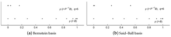
Figure 1.
Spectral distributions of matrices and in Example 1.
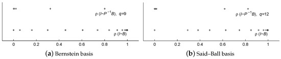
Figure 2.
Spectral distributions of matrices and in Example 2.
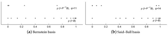
Figure 3.
Spectral distributions of matrices and in Example 3.
To further illustrate the effectiveness of the PPIA, we list in Table 1 the spectral radii of the iteration matrices of the WPIA, DWPIA and PPIA formats resulting from the considered Bézier and Said–Ball curves. Clearly, the spectral radii of the iteration matrices of the PPIA are much less than those of the corresponding WPIA, DWPIA. Additionally, we see that the spectral radii of PPIA decline sharply when the half-bandwidth of the preconditioner P is near . Those results entirely coincide with the aforementioned conclusions in Section 2. Therefore, we can expect that the PPIA method has a good convergence behavior.

Table 1.
The spectral radii of iteration matrices of WPIA, DWPIA and PPIA in Examples 1–3.
We denote the number of iterations by k, the k-th interpolation error by and the elapsed CPU time after k iterations by (in seconds), respectively. We emphasize here that the elapsed CPU time for the same routine in Matlab was different every time. Therefore, we took the average of all runtimes of 100 independent runs as the elapsed CPU time. The detailed numerical results of the PPIA, DWPIA and WPIA resulting from Bézier curves and Said–Ball curves are listed in Table 2, Table 3 and Table 4, respectively. Under the requirement of the same precision, the number of iterations by PPIA is much less than those of WPIA and DWPIA, and the runtime by PPIA is much less than the runtimes of WPIA and DWPIA. This means that our PPIA can accelerate the convergence rate of PIA significantly.
Table 2.
The approximation errors and runtimes of WPIA, DWPIA and PPIA in Example 1.
Table 3.
The approximation errors and runtime of WPIA, DWPIA and PPIA in Example 2.
Table 4.
The approximation errors and runtime of WPIA, DWPIA and PPIA in Example 3.
In Table 5, we show the detailed runtimes of WPIA, DWPIA and PPIA for when we tested Example 3 by using Bézier curves and Said–Ball curves. We denote the runtime of computing the optimal weight for WPIA by , the runtime of computing different weights for DWPIA by and the runtime of constructing the preconditioner P for PPIA by , respectively. We can see that the cost of constructing P is small enough and can be neglected.
Table 5.
The detailed runtime of WPIA, DWPIA and PPIA in Example 3.
We remark here that all curves in Figure 4, Figure 5 and Figure 6 are those obtained at 10th iteration step by employing different iterations with different bases, respectively. In Figure 4, Figure 5 and Figure 6, the curves generated by PPIA and WPIA formats are denoted by the solid and dashed lines respectively. We can see from Figure 4, Figure 5 and Figure 6 that the approximations obtained by PPIA are better than those obtained by WPIA, no matter whether Bézier curves or Said–Ball curves are used. Clearly, the PPIA converges faster than the WPIA.
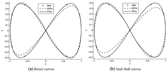
Figure 4.
Approximations of the lemniscate of Gerono in Example 1 at the tenth iteration.
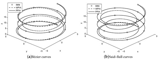
Figure 5.
Approximations of the helix in Example 2 at the tenth iteration.
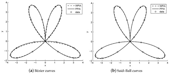
Figure 6.
Approximations of the four-leaf clover in Example 3 at the tenth iteration.
4.2. Tests for IPPIA
From the above numerical experiments, we know that the PPIA works much better than the WPIA and DWPIA if the number of the interpolating points is moderate. However, when we fit 53 points sampled from the lemniscate of Gerono, the helix and the four-leaf clover in Examples 1–3 by using Bézier curves and Said–Ball curves, we found that the WPIA and DWPIA converge very slowly. At the same time, we found that the PPIA does not work, because the condition number of P is very large and the solution to cannot be directly obtained. In this case, we can employ the IPPIA to get the corresponding fitting curves. The numerical results (including the number of iterations, the approximation errors and the runtime) obtained by the WPIA, DWPIA and IPPIA are listed in Table 6, Table 7 and Table 8 respectively, where the parameters in IPPIA are taken as , and .
Table 6.
Numerical results when fitting 53 points sampled from the lemniscate of Gerono.
Table 7.
Numerical results when fitting 53 points sampled from the helix.
Table 8.
Numerical results when fitting 53 points sampled from the four-leaf clover.
From Table 6, Table 7 and Table 8, we can see that the IPPIA converges much faster than the WPIA and DWPIA. For example, when we fit the points sampled from the lemniscate of Gerono by using Bézier curves, we observed that the errors caused by performing 5 IPPIA iterations are about the same as those caused by performing 137 WPIA iterations or 381 DWPIA iterations. Again, when we fit 53 points sampled from the lemniscate of Gerono by using Said–Ball curves, we found that the errors caused by performing 4 IPPIA iterations are about the same as those caused by performing 291 WPIA iterations or 358 DWPIA iterations. Furthermore, under the requirement of the same accuracy, the runtime of IPPIA iterations was less than that of WPIA iterations and it was comparable to that of DWPIA iterations.
When fitting 53 points sampled from the lemniscates of Gerono, helix and four-leaf clover, we sketched the Bézier curves and the Said–Ball curves generated by performing five IPPIA and WPIA iterations in Figure 7, Figure 8 and Figure 9, respectively. The solid and dashed lines in Figure 7, Figure 8 and Figure 9 represent the curves generated by IPPIA and WPIA respectively. Clearly, the IPPIA outperforms the WPIA in the sense of the convergence rate.
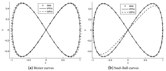
Figure 7.
Approximations to 53 points sampled from the lemniscate of Gerono at the fifth iteration.
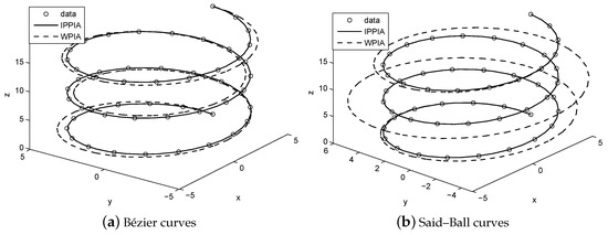
Figure 8.
Approximations of 53 points sampled from the helix at the fifth iteration.
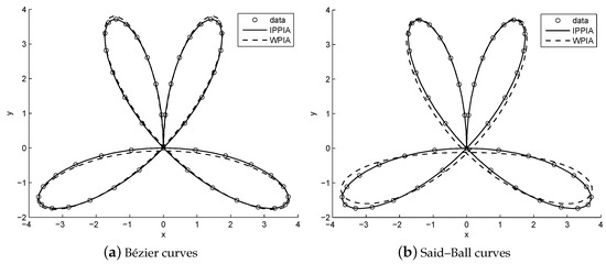
Figure 9.
Approximations of 53 points sampled from the four-leaf clover at the fifth iteration.
5. Conclusions
In this paper, we have exploited the properties of collocation matrix B, resulting from an NTP basis, to design an efficient preconditioner P for PIA. The main tool to derive our preconditioner is the diagonally compensated reduction. By applying that P to PIA, we have developed a novel version of PIA, called the PPIA. By both convergence theory and numerical experiments, we have shown that the PPIA outperforms the WPIA and DWPIA, in the sense of convergence rate and elapsed CPU time. In particular, to reduce the computational complexity of PPIA, we have also proposed an inexact variant of PPIA (i.e., IPPIA) and shown its effectiveness, especially when the number of interpolating points is large.
As mentioned in Section 1, the PIA has extensive successful applications. Therefore, we can expect that our methods have a wide range of potential applications.
Author Contributions
Methodology, Z.L.; Resources, C.L.; Writing—original draft, C.L.; Writing—review and editing, Z.L. All authors have read and agreed to the published version of the manuscript.
Funding
This research was funded by the National Natural Science Foundation of China (grant numbers 11371075 and 11771453), the Hunan Key Laboratory of mathematical modeling and analysis in engineering, Natural Science Foundation of Hunan Province (grant number 2020JJ5267) and the Scientific Research Funds of Hunan Provincial Education Department (grant number 18C877).
Conflicts of Interest
The authors declare no conflict of interest.
References
- Hu, Q. An iterative algorithm for polynomial of rational triangular Bézier surfaces. Appl. Math. Comput. 2013, 219, 9308–9316. [Google Scholar] [CrossRef]
- Gofuku, S.; Tamura, S.; Maekawa, T. Point-tangent/point-normal B-spline curve interpolation by geometric algorithms. Comput. Aided Des. 2009, 41, 412–422. [Google Scholar] [CrossRef]
- Lin, H. Adaptive data fitting by the progressive-iterative approximation. Comput. Aided Geom. Des. 2012, 29, 463–473. [Google Scholar] [CrossRef]
- Lin, H.; Zhang, Z. An efficient method for fitting large data sets using T-splines. SIAM J. Sci. Comput. 2013, 35, 3052–3068. [Google Scholar] [CrossRef]
- Kineri, Y.; Wang, M.; Lin, H.; Maekawa, T. B-spline surface fitting by iterative geometric interpolation/ approximation algorithms. Comput. Aided Des. 2012, 44, 697–708. [Google Scholar] [CrossRef]
- Lin, H.; Jin, S.; Liao, H.; Jian, Q. Quality guaranteed all-hex mesh generation by a constrained volume iterative fitting algorithm. Comput. Aided Des. 2015, 67, 107–117. [Google Scholar] [CrossRef]
- Martin, T.; Cohen, E.; Kirby, R. Volumetric parameterization and trivariate B-spline fitting using harmonic functions. Comput. Aided Geom. Des. 2009, 26, 648–664. [Google Scholar] [CrossRef]
- Lin, H.; Jin, S.; Hu, Q.; Liu, Z. Constructing B-spline solids from tetrahedral meshes for isogeometric analysis. Comput. Aided Geom. Des. 2015, 3, 109–120. [Google Scholar] [CrossRef]
- Lin, H.; Maekawa, T.; Deng, C. Survey on geometric iterative methods and their applications. Comput. Aided Des. 2017, 95, 40–51. [Google Scholar] [CrossRef]
- Marco, A.; Martínez, J. A fast and accurate algorithm for solving Bernstein-Vandermonde linear systems. Linear Algebra Appl. 2006, 2, 616–628. [Google Scholar] [CrossRef]
- Deng, S.; Wang, G. Numerical analysis of the progressive iterative approximation method. Comput. Aided Des. Graph. 2012, 7, 879–884. [Google Scholar]
- Lu, L. Weighted progressive iteration approximation and convergence analysis. Comput. Aided Geom. Des. 2010, 2, 129–137. [Google Scholar] [CrossRef]
- Carnicer, J.M.; Delgado, J.; Pena, J. Richardson method and totally nonnegative linear systems. Linear Algebra Appl. 2010, 11, 2010–2017. [Google Scholar] [CrossRef]
- Liu, X.; Deng, C. Jacobi-PIA algorithm for non-uniform cubic B-Spline curve interpolation. J. Comput. Aided Des. Comput. Graph. 2015, 27, 485–491. [Google Scholar]
- Liu, C.; Han, X.; Li, J. The Chebyshev accelerating method for progressive iterative approximation. Commun. Inf. Syst. 2017, 17, 25–43. [Google Scholar] [CrossRef]
- Zhang, L.; Zhao, L.; Tan, J. Progressive iterative approximation with different weights and its application. J. Zhejiang Univ. Sci. Ed. 2017, 44, 22–27. [Google Scholar]
- Wang, Z.; Li, J.; Deng, C. Convergence proof of GS-PIA algorithm. J. Comput. Aided Des. Comput. Graph. 2018, 30, 60–66. [Google Scholar] [CrossRef]
- Zhang, L.; Tan, J.; Ge, X.; Guo, Z. Generalized B-splines’ geometric iterative fitting method with mutually different weights. J. Comput. Appl. Math. 2018, 329, 331–343. [Google Scholar] [CrossRef]
- Ebrahimi, A.; Loghmani, G. A composite iterative procedure with fast convergence rate for the progressive-iteration approximation of curves. J. Comput. Appl. Math. 2019, 359, 1–15. [Google Scholar] [CrossRef]
- Lin, H. Local progressive-iterative approximation format for blending curves and patches. Comput. Aided Geom. Des. 2010, 27, 322–339. [Google Scholar] [CrossRef]
- Lin, H.; Zhang, Z. An extended iterative format for the progressive-iteration approximation. Comput. Graph. 2011, 35, 967–975. [Google Scholar] [CrossRef]
- Deng, C.; Lin, H. Progressive and iterative approximation for least squares B-spline curve and surface fitting. Comput. Aided Des. 2014, 47, 32–44. [Google Scholar] [CrossRef]
- Farouki, R. The Bernstein polynomial basis: A centennial retrospective. Comput. Aided Geom. Des. 2012, 29, 379–419. [Google Scholar] [CrossRef]
- Delgado, J.; Pena, J. On the generalized Ball bases. Adv. Comput. Math. 2006, 24, 263–280. [Google Scholar] [CrossRef]
- Lin, H.; Bao, H.; Wang, G. Totally positive bases and progressive iteration approximation. Comput. Math. Appl. 2005, 50, 575–586. [Google Scholar] [CrossRef]
- Carnicer, J.M.; Delgado, J. On the progressive iteration approximation property and alternative iterations. Comput. Aided Geom. Des. 2011, 28, 523–526. [Google Scholar] [CrossRef]
- Liu, Z.; Wu, N.; Qin, X.; Zhang, Y. Trigonometric transform splitting methods for real symmetric Toeplitz systems. Comput. Math. Appl. 2018, 75, 2782–2794. [Google Scholar] [CrossRef]
- Liu, Z.; Qin, X.; Wu, N.; Zhang, Y. The shifted classical circulant and skew circulant splitting iterative methods for Toeplitz matrices. Canad. Math. Bull. 2017, 60, 807–815. [Google Scholar] [CrossRef]
- Liu, Z.; Ralha, R.; Zhang, Y.; Ferreira, C. Minimization problems for certain structured matrices. Electron. J. Linear Algebra 2015, 30, 613–631. [Google Scholar] [CrossRef][Green Version]
- Axelsson, O. Iterative Solution Methods; Cambridge University Press: Cambridge, UK, 1994. [Google Scholar]
- Cao, Z.; Liu, Z. Symmetric multisplitting of a symmetric positive definite matrix. Linear Algebra Appl. 1998, 285, 309–319. [Google Scholar] [CrossRef]
© 2020 by the authors. Licensee MDPI, Basel, Switzerland. This article is an open access article distributed under the terms and conditions of the Creative Commons Attribution (CC BY) license (http://creativecommons.org/licenses/by/4.0/).