The Convergence Analysis of a Numerical Method for a Structured Consumer-Resource Model with Delay in the Resource Evolution Rate

Abstract

In this paper, we go through the development of a new numerical method to obtain the solution to a size-structured population model that describes the evolution of a consumer feeding on a dynamical resource that reacts to the environment with a lag-time response. The problem involves the coupling of the partial differential equation that represents the population evolution and an ordinary differential equation with a constant delay that describes the evolution of the resource. The numerical treatment of this problem has not been considered before when a delay is included in the resource evolution rate. We analyzed the numerical scheme and proved a second-order rate of convergence by assuming enough regularity of the solution. We numerically confirmed the theoretical results with an academic test problem.

1. Introduction

We consider a model that describes the evolution of a size-structured consumer in an environment inhabited by a single unstructured resource. We assume that the resource responds to the environment with a constant time delay. The model is composed of two nonlinear coupled problems. On the one hand, a size-structured population model governed by a first-order hyperbolic equation with a nonlocal and nonlinear boundary condition, which represents the evolution over time of the consumer:

$$\left\{\begin{array}{cc}\hfill & u_t+{\left(g(x,s\left(t\right),t)u\right)}_x=-\mu (x,s\left(t\right),t)u,x_0<x<x_M\left(t\right),t>0,\hfill \\ \hfill & {\displaystyle g(x_0,s\left(t\right),t)u(x_0,t)={\int }_{x_0}^{x_M\left(t\right)}\alpha (x,s\left(t\right),t)u(x,t)dx,t>0,}\hfill \\ \hfill & u(x,0)=u_0\left(x\right),x_0\le x\le x_M^0.\hfill \end{array}\right.$$

(1)

Variables x and t represent the size and the time, respectively. Size is the variable which structures the individuals in the consumer population, $x_0$ denotes the newborn individual’s size (the size at birth) that is assumed to be constant and positive and $x_M\left(t\right)$ represents the maximum size of individuals at time t. Then, $x_M\left(0\right)=x_M^0$ is the initial maximum size. The dependent variables u and s are the density of individuals of size x and the amount of the resource available at time t, respectively. The so-called vital rates, the mortality, the fertility and the growth rates, are given by $\mu$, $\alpha$ and g, respectively. The mortality and the fertility are nonnegative functions and the growth rate has no-sign restriction, although we assume that $g(x_0,·,·)>0$, which means that each individual increases in size at birth. Vital rates depend on the structuring variable, the time and the amount of the resource available, to take into account the influences of these factors on the dynamics of the population. The size of the individuals changes according to the differential equation

$$x^{\prime }\left(t\right)=g(x\left(t\right),s\left(t\right),t),t>0.$$

As we allow a negative growth rate g, we are considering the case in which an individual in the population could shrink in size under a food shortage environmental condition. In particular, the maximum size, $x_M\left(t\right)$, is not fixed in the model and evolves following the corresponding characteristic curve of (1)

$$\left\{\begin{array}{c}{x}_M^{\prime }\left(t\right)=g(x_M\left(t\right),s\left(t\right),t),t>0,\hfill \\ x_M\left(0\right)=x_M^0.\hfill \end{array}\right.$$

(2)

On the other hand, the unstructured resource $s\left(t\right)$, $t\ge 0$, which provides feeding for the individuals of the population, evolves with time according to the following initial value problem for a delay ordinary differential equation:

$$\left\{\begin{array}{c}{s}^{\prime }\left(t\right)=f(s\left(t\right),s(t-\tau ),I\left(t\right),t),t>0,\hfill \\ s\left(t\right)=s_0\left(t\right),t\in [-\tau ,0].\hfill \end{array}\right.$$

(3)

The rate of change in the evolution of the resource is given by a function f that includes dependence on time and on the consumer population through the nonlocal term

$${\displaystyle I\left(t\right)={\int }_{x_0}^{x_M\left(t\right)}\gamma (x,s\left(t\right),t)u(x,t)dx,t\ge 0,}$$

(4)

where $\gamma$ is a function that represents the individual rate of consumption for individuals of a determined size. It also depends on the amount of the resource available at times t and $t-\tau$, $s\left(t\right)$ and $s(t-\tau )$ respectively. The memory effect, $s(t-\tau )$, can be seen as a deferred influence on the environment of the resource affordability. A common biological situation for this phenomenon occurs when the resource population is close to the carrying capacity of the environment or near extinction, which can make the population react with a certain delay [1]. Another situation in which this deferred influence occurs is when the resource is formed only by the adult individuals of the population, and the delay is due to the maturation time [2]. The solution of the model (1), (3) is determined once we know the initial conditions $u(x,0)=u_0\left(x\right)$, $x_0\le x\le x_M^0$, and $s\left(t\right)=s_0\left(t\right)$, $t\in [-\tau ,0]$.

Although a large number of papers on consumer models have been considered in past years, not so many address the case in which one of the populations is structured. Consumer-resource models have been studied from the very initial work of Kooijman and Metz [2]. These authors presented a mathematical model for the development of an ectothermic population (Daphnia magna, water flea) in which the amount of food they are supplied with represents a regulatory mechanism for the population density. The model was length-structured and also included a stage of maturity: a differentiation among juveniles and adults. This work is considered as the origin of the modern dynamic energy budget theory. The well-posedness of the model equations and the continuously dependence on model data was studied by Thieme [3]. The dynamical properties of the model were explored numerically in [4], and later, analytically in [5,6,7]. However the description of the evolution of the resource as a delay differential equation within a physiological structured consumer-resource model has not been developed theoretically yet.

The theoretical treatment of this model is not easy; therefore, its numerical analysis is a valid tool and sometimes the only one affordable. The integration of the model without delay has been developed by means of the Excalator Boxcar Train (EBT) [8] and a characteristics method [9]. This last work included the convergence proof of the method while the convergence of the popular EBT method was recently considered [10,11]. However, the numerical treatment of the coupled model with a resource evolving according to a delay differential equation remained unexplored until our study, so our goal was to provide a numerical method to perform the integration of such a model and its convergence analysis.

The remainder of the paper is organized as follows. Section 2 is devoted to the introduction of the numerical method to integrate problem (1), (3). We employ the technique of integration along the characteristic curves in order to obtain the new numerical scheme. In Section 3, we carry out the convergence analysis of the scheme. It is based on a theoretical framework that involves the properties of consistency and stability of the numerical method. We also pay attention to the properties required by the numerical quadrature rule used in the integration. Finally, in Section 4, we present a test done in order to numerically confirm the theoretical order of convergence.

2. Numerical Method

We begin with the description of the numerical scheme. We must employ the integration along the characteristic curves; therefore, we should remind the reader of the definition of $x(t;t^{*},x_{*})$, $x_{*}\in [x_0,x_M\left(t\right)]$, $t^{*}>0$, as the solution of

$$\left\{\begin{array}{c}{\displaystyle \frac{d}{dt}x(t;t^{*},x_{*})=g(x(t;t^{*},x_{*}),s\left(t\right),t),t\ge t^{*},}\hfill \\ x(t^{*};t^{*},x_{*})=x_{*},\hfill \end{array}\right.$$

(5)

that represents the characteristic curve that at time $t^{*}$ starts at $x_{*}$. Now, we consider $w(t;t^{*},x_{*})=u(x(t;t^{*},x_{*}),t)$, for each $x_{*}\in [x_0,x_M\left(t\right)]$, $t^{*}>0$. It satisfies the following initial value problem

$$\left\{\begin{array}{cc}\hfill & {\displaystyle \frac{d}{dt}w(t;t^{*},x_{*})=-{\mu }^{*}(x(t;t^{*},x_{*}),s\left(t\right),t)w(t;t^{*},x_{*}),t>t^{*},}\hfill \\ \hfill & w(t^{*};t^{*},x_{*})=u(x_{*},t^{*}),\hfill \end{array}\right.$$

(6)

where ${\mu }^{*}(x,s\left(t\right),t)=\mu (x,s\left(t\right),t)+g_x(x,s\left(t\right),t)$, whose solution is given by the following formula

$$u(x(t;t^{*},x_{*}),t)=u(x_{*},t^{*})exp\left\{{\displaystyle -{\int }_{t^{*}}^t{\mu }^{*}\left(x\left(\varpi ;t^{*},x_{*}\right),s\left(\varpi \right),\varpi \right)d\varpi }\right\},t\ge t^{*}.$$

(7)

For the numerical method, we discretize this expression, together with the boundary condition and the initial data in (1), and the initial value problem in (3).

The integration is carried out on a finite time interval $[0,T]$. Then, given $J,L\in \mathbb{N}$, we define the discretization parameters $h=(x_M^0-x_0)/J$, $k=\tau /L$, and the number of discrete time levels $N=[T/k]$, which are given by $t^n=nk$, $-L\le n\le N$. We begin the description of the numerical method with the initial values, which, in this case, are the initial size discretization ${\mathbf{X}}^0$, $X_j^0=x_0+jh$, $0\le j\le J$, the  initial condition on the initial grid, ${\mathbf{U}}^0$, $U_j^0=u_0\left(X_j^0\right)$, $0\le j\le J$, and the resource, that has to be initialized on the interval $[-\tau ,0]$, with the values $S^n=s_0\left(t^n\right)$, $-L\le n\le 0$.

We compute, for $0\le n\le N-1$, the approximation at the general level $t^{n+1}$: $\{{\mathbf{X}}^{n+1}$, $S^{n+1}$, ${\mathbf{U}}^{n+1}\}$, ${\mathbf{X}}^{n+1}=(X_0^{n+1},X_1^{n+1},\dots ,X_{J+n+1}^{n+1})$, ${\mathbf{U}}^{n+1}=(U_0^{n+1},U_1^{n+1},\dots ,U_{J+n+1}^{n+1})$ when the values at the previous time steps are known: $\{{\mathbf{X}}^m$, $S^m$, ${\mathbf{U}}^m\}$, ${\mathbf{X}}^m=(X_0^m,X_1^m,\dots ,X_{J+m}^m)$, ${\mathbf{U}}^m=(U_0^m,U_1^m,\dots ,U_{J+m}^m)$, $0\le m\le n$. We should point out that we design a second-order method based on the modified Euler scheme and on the trapezoidal quadrature rule. This means that we need an intermediate stage in which we compute a first-order approximation: $\{{\mathbf{X}}^{n+1,*}$, $S^{n+1,*}$, ${\mathbf{U}}^{n+1,*}\}$, ${\mathbf{X}}^{n+1,*}=(X_0^{n+1,*},X_1^{n+1,*},\dots ,X_{J+n+1}^{n+1,*})$, ${\mathbf{U}}^{n+1,*}=(U_0^{n+1,*},U_1^{n+1,*},\dots ,U_{J+n+1}^{n+1,*})$, given by the equations

$$\left\{\begin{array}{c}{X}_0^{n+1,*}=x_0,X_{j+1}^{n+1,*}=X_j^n+kg(X_j^n,S^n,t^n),0\le j\le J+n,\hfill \\ S^{n+1,*}=S^n+kf(S^n,S^{n-L},\mathcal{Q}({\mathbf{X}}^n,{\mathbf{\gamma }}^n\left(\mathbf{X},S\right)·{\mathbf{U}}^n),t^n),\hfill \\ U_{j+1}^{n+1,*}=U_j^{n}exp\left\{-k{\mu }^{*}(X_j^n,S^n,t^n)\right\},0\le j\le J+n,\hfill \\ g(X_0^{n+1,*},S^{n+1,*},t^{n+1})U_0^{n+1,*}=\mathcal{Q}({\mathbf{X}}^{n+1,*},{\mathbf{\alpha }}^{n+1,*}\left(\mathbf{X},S\right)·{\mathbf{U}}^{n+1,*}).\hfill \end{array}\right.$$

(8)

As soon as we have computed the intermedium quantities $\{{\mathbf{X}}^{n+1,*}$, $S^{n+1,*}$, ${\mathbf{U}}^{n+1,*}\}$ we can obtain the approximations at the advanced time level with

$$\left\{\begin{array}{c}{\displaystyle X_0^{n+1}=x_0,X_{j+1}^{n+1}=X_j^n+\frac{k}{2}\left(g(X_j^n,S^n,t^n)+g(X_{j+1}^{n+1,*},S^{n+1,*},t^{n+1})\right),0\le j\le J+n,}\hfill \\ {\displaystyle S^{n+1}=S^n+\frac{k}{2}\left(f(S^n,S^{n-L},\mathcal{Q}({\mathbf{X}}^n,{\mathbf{\gamma }}^n\left(\mathbf{X},S\right)·{\mathbf{U}}^n),t^n)\right.}\hfill \\ +\left.f(S^{n+1,*},S^{n+1-L},\mathcal{Q}({\mathbf{X}}^{n+1,*},{\mathbf{\gamma }}^{n+1,*}\left(\mathbf{X},S\right)·{\mathbf{U}}^{n+1,*}),t^{n+1})\right),\hfill \\ U_{j+1}^{n+1}=U_j^{n}exp\left\{{\displaystyle -\frac{k}{2}\left({\mu }^{*}(X_j^n,S^n,t^n)+{\mu }^{*}(X_{j+1}^{n+1,*},S^{n+1,*},t^{n+1})\right)}\right\},0\le j\le J+n,\hfill \\ g(X_0^{n+1},S^{n+1},t^{n+1})U_0^{n+1}=\mathcal{Q}({\mathbf{X}}^{n+1},{\mathbf{\alpha }}^{n+1}\left(\mathbf{X},S\right)·{\mathbf{U}}^{n+1}).\hfill \end{array}\right.$$

(9)

In (8) and (9), at each time level, ${\mathbf{\gamma }}^n\left(\mathbf{X},S\right)$ and ${\mathbf{\alpha }}^n\left(\mathbf{X},S\right)$ represent vectors with components ${\mathbf{\gamma }}_j^n\left(\mathbf{X},S\right)=\gamma (X_j^n,S^n,t^n)$ and ${\mathbf{\alpha }}_j^n\left(\mathbf{X},S\right)=\alpha (X_j^n,S^n,t^n)$, $0\le j\le J+n$, respectively, and ${\mathbf{\gamma }}^{n,*}\left(\mathbf{X},S\right)$ and ${\mathbf{\alpha }}^{n,*}\left(\mathbf{X},S\right)$ vectors with components ${\mathbf{\gamma }}_j^{n,*}\left(\mathbf{X},S\right)=\gamma (X_j^{n,*},S^{n,*},t^n)$ and ${\mathbf{\alpha }}_j^{n,*}\left(\mathbf{X},S\right)=\alpha (X_j^{n,*},S^{n,*},t^n)$, $0\le j\le J+n+1$, respectively. The notation ${\mathbf{\gamma }}^n\left(\mathbf{X},S\right)·{\mathbf{U}}^n$, ${\mathbf{\alpha }}^n\left(\mathbf{X},S\right)·{\mathbf{U}}^n$, ${\mathbf{\gamma }}^{n,*}\left(\mathbf{X},S\right)·{\mathbf{U}}^{n,*}$ and ${\mathbf{\alpha }}^{n,*}\left(\mathbf{X},S\right)·{\mathbf{U}}^{n,*}$ represent the componentwise products of the corresponding vectors, and $\mathcal{Q}$ is an appropriate second-order quadrature rule, as given below. We observed that, in this procedure, the total number of nodes in the grid increases in one at each time step due to the new node that fluxes from the left boundary into the domain. This feature led us to name this kind of scheme the aggregation grid nodes method (AGN) [12]. The algorithm is explicit and totally straightforward and can be resumed as in the pseudocode given in Box 1.

Box 1. Pseudocode of the algorithm AGN (and SGN).

% Choose L, J integers

$k=\tau /L$; $h=(x_M^0-x_0)/J$

$N=[T/k]$

% Initialization

do j=0,J

   $X_j^0=x_0+jh$ % Initial grid points

   $U_j^0=u_0\left(X_j^0\right)$

end

do n=-L,0

   $S^n=s_0\left(t^n\right)$

end

% Advancing the solution on time, step by step

do n=0, N-1

   Formulae in (8) % First stage to ${\mathbf{X}}^{n+1,*}$, $S^{n+1,*}$, ${\mathbf{U}}^{n+1,*}$

   Formulae in (9) % Second stage to ${\mathbf{X}}^{n+1}$, $S^{n+1}$, ${\mathbf{U}}^{n+1}$

% Optional (difference between AGN and SGN methods)

   Formulae in (10) % Selection procedure in case of SGN method

end

In the numerical experimentation, we use a more efficient procedure in order to keep the number of nodes constant (and consequently, to not increase the computational cost) at each time step. Toward that goal, we eliminate a chosen node from the grid at each time step. The selection procedure we use in the method depends on the dynamics of the grid, as it was introduced in [13]. We refer to this kind of scheme as the selection grid nodes method (SGN) [12]. The node picked out is the first $X_l^{n+1}$ that satisfies

$$|X_{l+1}^{n+1}-X_{l-1}^{n+1}|=\underset{1\le j\le J}{min}|X_{j+1}^{n+1}-X_{j-1}^{n+1}|.$$

(10)

Once it is elected, we rename the nodes to keep the index labels from $j=0$ to $j=J$.

Finally, we pay attention to the nonlocal terms; they are discretized by means of a composite quadrature rule, based on the trapezoidal formula, on the grid points $\mathbf{X}=(X_0,X_1,\dots ,X_{\aleph })$, $\aleph \in \mathbb{N}$,

$${\displaystyle \mathcal{Q}(\mathbf{X},\mathbf{V})=\sum _{l=0}^{\aleph -1}\frac{X_{l+1}-X_l}{2}(V_l+V_{l+1}),\mathrm{where}\mathbf{V}=(V_0,V_1,\dots ,V_{\aleph }).}$$

3. Convergence Analysis

The convergence analysis here follows the discretization framework developed in [14]. In this framework, suitable discrete normed spaces and operators are introduced to formulate the equations of the numerical method. Then, appropriate properties of consistency and nonlinear stability are established. The numerical method is an adaptation of the one given in [9], and so is the analysis. However, for the sake of completeness, we provide the details of the numerical method formulation, and for the sake of simplicity, we present only those parts of the convergence analysis proofs associated with estimates derived from the discretization of the delay term in the differential equation. That means that the step by step recurrences for the errors at each time level increase the order of the difference equation as the time discretization parameter tends to zero. For the theoretical analysis, we consider the AGN method.

With this aim, we fix $T>0$ and assume that the problem (1), (3) has a unique solution $u(x,t)$, $x\in [x_0,x_M\left(t\right)]$, and $s\left(t\right)$, $t\in [-\tau ,T]$, with the following regularity assumptions:

Hypothesis 1 (H1).

$u\in {\mathcal{C}}^2([x_0,x_M\left(t\right)]\times [0,T])$ and is nonnegative.

Hypothesis 2 (H2).

$s\in {\mathcal{C}}^2\left([-\tau ,T]\right)$ and is nonnegative.

Additionally, we assume that there exists a compact neighborhood D of ${\displaystyle \left\{s\left(t\right),0\le t\le T\right\}}$, such that

Hypothesis 3 (H3).

$\gamma \in {\mathcal{C}}^2([x_0,x_M\left(t\right)]\times D\times [0,T])$ and is nonnegative.

Hypothesis 4 (H4).

$\mu \in {\mathcal{C}}^2([x_0,x_M\left(t\right)]\times D\times [0,T])$ and is nonnegative.

Hypothesis 5 (H5).

$\alpha \in {\mathcal{C}}^2([x_0,x_M\left(t\right)]\times D\times [0,T])$ and is nonnegative.

Hypothesis 6 (H6).

$g\in {\mathcal{C}}^3([x_0,x_M\left(t\right)]\times D\times [0,T])$ and there exists a positive constant C such that $g(x_0,s,t)\ge C$, $s,t\ge 0$. In addition, the characteristic curves $x(t;t^{*},x_{*})$ defined by (5), are continuous and differentiable with respect to the initial values $(t^{*},x_{*})\in [0,T]\times [x_0,x_M\left(t\right)]$.

Finally, we suppose that there are compact neighborhoods, $D_f$ of ${\displaystyle \left\{s\left(t\right),-\tau \le t\le T\right\}}$, and $D_I$ of ${\displaystyle \left\{{\int }_{x_0}^{x_M\left(t\right)}\gamma (x,s\left(t\right),t)u(x,t)dx,0\le t\le T\right\}}$, such that

Hypothesis 7 (H7).

$f\in {\mathcal{C}}^2(D_f\times D_f\times D_I\times [0,T])$ and is nonnegative.

Now, we choose $L\in \mathbb{N}$ and assume that the time discretization parameter, k, takes values in the set

$$K=\{k:k=\tau /(\nu L),\nu \in \mathbb{N}\}.$$

Then for $k\in K$, we set $N=[T/k]$ and choose $J\in \mathbb{N}$ such that $h=(x_M^0-x_0)/J$, and the ratio $r:=k/h$ is a positive constant fixed throughout the analysis. Then, $x_M^0$ is always the last node in the size grid. For each $k\in K$, we define the space

$${\mathcal{A}}_k=\prod _{n=0}^N\left({\mathbb{R}}^{J+n}\times {\mathbb{R}}^{J+n+1}\right)\times {\mathbb{R}}^{L+N+1},$$

where vectors $\left({\mathbf{y}}^0,{\mathbf{V}}^0,\dots ,{\mathbf{y}}^N,{\mathbf{V}}^N,\mathbf{a}\right)\in {\mathcal{A}}_k$ are used to describe the following approximations: to the inner and right-hand boundary grid nodes, given by ${\mathbf{y}}^n\in {\mathbb{R}}^{J+n}$, and to the theoretical solution at the complete grid, ${\mathbf{V}}^n\in {\mathbb{R}}^{J+n+1}$, for each time level $t^n$, $0\le n\le N$; and to the theoretical solution to the delay differential equation at time levels $t^n$, $-L\le n\le N$, provided by $\mathbf{a}\in {\mathbb{R}}^{L+N+1}$. We also consider the space

$${\mathcal{B}}_k=\left({\mathbb{R}}^J\times {\mathbb{R}}^{J+1}\times {\mathbb{R}}^{L+1}\right)\times {\mathbb{R}}^N\times \prod _{n=1}^N\left({\mathbb{R}}^{J+n}\times {\mathbb{R}}^{J+n}\right)\times {\mathbb{R}}^N,$$

where each component of vector $\left({\mathbf{Y}}^0,{\mathbf{P}}^0,{\mathbf{A}}^0,{\mathbf{P}}_0,{\mathbf{Y}}^1,{\mathbf{P}}^1,\dots ,{\mathbf{Y}}^N,{\mathbf{P}}^N,\mathbf{A}\right)\in {\mathcal{B}}_k$ describes the residuals of the discrete solution when it is substituted on the discrete equations that define the numerical method: we discriminate ${\mathbf{Y}}^0$, ${\mathbf{P}}^0$, ${\mathbf{A}}^0=(A^{-L},A^{-L+1},\dots ,A^0)$, given by the approximations to the initial conditions; ${\mathbf{P}}_0$, provided by the solution at the left boundary node at each time level; ${\mathbf{Y}}^n$, ${\mathbf{P}}^n$, $0\le n\le N$, given by the grid nodes and solution to them; and $\mathbf{A}=(A^1,A^2,\dots ,A^N)$, due to the solution to the delay differential equation, as we show below. Both spaces, ${\mathcal{A}}_k$ and ${\mathcal{B}}_k$, have the same dimension.

In order to measure the size of the errors, we define

$${\parallel \mathbf{\eta }\parallel }_{\infty }=\underset{1\le j\le \aleph }{max}|{\eta }_j|,\mathbf{\eta }=({\eta }_1,{\eta }_2,\dots ,{\eta }_{\aleph })\in {\mathbb{R}}^{\aleph },$$

$${\parallel {\mathbf{V}}^n\parallel }_1=\sum _{j=0}^{J+n}h\left|V_j^n\right|,{\mathbf{V}}^n=(V_0^n,V_1^n,\dots ,V_{J+n}^n)\in {\mathbb{R}}^{J+n+1}.$$

Thus, we endow the spaces ${\mathcal{A}}_k$ and ${\mathcal{B}}_k$ with the following norms. If $\left({\mathbf{y}}^0,{\mathbf{V}}^0,\dots ,{\mathbf{y}}^N,{\mathbf{V}}^N,\mathbf{a}\right)\in {\mathcal{A}}_k$,

$${\parallel \left({\mathbf{y}}^0,{\mathbf{V}}^0,\dots ,{\mathbf{y}}^N,{\mathbf{V}}^N,\mathbf{a}\right)\parallel }_{{\mathcal{A}}_k}=max\left(\underset{0\le n\le N}{max}\parallel {\mathbf{y}}^n{\parallel }_{\infty },\underset{0\le n\le N}{max}\parallel {\mathbf{V}}^n{\parallel }_{\infty },{\parallel \mathbf{a}\parallel }_{\infty }\right).$$

On the other hand, if $\left({\mathbf{Y}}^0,{\mathbf{P}}^0,{\mathbf{A}}^0,{\mathbf{P}}_0,{\mathbf{Y}}^1,{\mathbf{P}}^1,\dots ,{\mathbf{Y}}^N,{\mathbf{P}}^N,\mathbf{A}\right)\in {\mathcal{B}}_k$,

$$\begin{array}{c}{\displaystyle \parallel \left({\mathbf{Y}}^0,{\mathbf{P}}^0,{\mathbf{A}}^0,{\mathbf{P}}_0,{\mathbf{Y}}^1,{\mathbf{P}}^1,\dots ,{\mathbf{Y}}^N,{\mathbf{P}}^N,\mathbf{A}\right){\parallel }_{{\mathcal{B}}_k}}\hfill \\ ={\parallel {\mathbf{Y}}^0\parallel }_{\infty }+\parallel {\mathbf{P}}^0{\parallel }_{\infty }+\parallel {\mathbf{A}}^0{\parallel }_{\infty }+\parallel {\mathbf{P}}_0{\parallel }_{\infty }+\sum _{n=1}^{N}k\parallel {\mathbf{Y}}^n{\parallel }_{\infty }+\sum _{n=1}^{N}k\parallel {\mathbf{P}}^n{\parallel }_{\infty }+\sum _{n=1}^{N}k\left|A^n\right|.\hfill \end{array}$$

Now, for each $k\in K$, we define

$${\mathbf{x}}^n=(x_1^n,\dots ,x_{J+n}^n)\in {\mathbb{R}}^{J+n},x_j^0=x_0+jh,1\le j\le J;x_j^n=x(t_n;t_{n-1},x_{j-1}^{n-1}),1\le j\le J+n,1\le n\le N;$$

(11)

and we denote $x_0^n=x_0$, $n\ge 0$. Recall that $x(t;t^{*},x_{*})$ represents the theoretical solution to problem (5), $t^{*}\in [0,T]$, $x^{*}\in [x_0,x_M\left(t\right)]$. In addition, if u represents the theoretical solution to (1) we define

$${\mathbf{u}}^n=(u_0^n,u_1^n,\dots ,u_{J+n}^n)\in {\mathbb{R}}^{J+n+1},u_j^n=u(x_j^n,t_n),0\le j\le J+n,0\le n\le N.$$

(12)

Finally, if s is the theoretical solution to (3) then we define

$${\mathbf{s}}_k=(s^{-L},s^{-L+1},\dots ,s^N),s^n=s\left(t^n\right),-L\le n\le N.$$

(13)

Therefore, ${\tilde{\mathbf{u}}}_k=({\mathbf{x}}^0,{\mathbf{u}}^0,{\mathbf{x}}^1,{\mathbf{u}}^1,\dots ,{\mathbf{x}}^N,{\mathbf{u}}^N,{\mathbf{s}}_k)\in {\mathcal{A}}_k$.

In the following, we introduce the discretization operator. Let R be a positive constant and let we denote by $B_{{\mathcal{A}}_k}({\tilde{\mathbf{u}}}_k,R{k}^p)\subset {\mathcal{A}}_k$ the open ball with center ${\tilde{\mathbf{u}}}_k$ and radius $R{k}^p$, $1<p<2$. Then, we define

$${\Phi }_k:B_{{\mathcal{A}}_k}({\tilde{\mathbf{u}}}_k,R{k}^p)\to {\mathcal{B}}_k,$$

$${\Phi }_k\left({\mathbf{y}}^0,{\mathbf{V}}^0,\dots ,{\mathbf{y}}^N,{\mathbf{V}}^N,\mathbf{a}\right)=\left({\mathbf{Y}}^0,{\mathbf{P}}^0,{\mathbf{A}}^0,{\mathbf{P}}_0,{\mathbf{Y}}^1,{\mathbf{P}}^1,\dots ,{\mathbf{Y}}^N,{\mathbf{P}}^N,\mathbf{A}\right),$$

(14)

given by the following equations, first

$${\mathbf{Y}}^0={\mathbf{y}}^0-{\mathbf{X}}^0\in {\mathbb{R}}^J,$$

(15)

$${\mathbf{P}}^0={\mathbf{V}}^0-{\mathbf{U}}^0\in {\mathbb{R}}^{J+1},$$

(16)

$${\mathbf{A}}^0={\mathbf{a}}^0-{\mathbf{S}}^0\in {\mathbb{R}}^{L+1},$$

(17)

where ${\mathbf{a}}^0=(a^{-L},a^{-L+1},\dots ,a^0)$. Vectors ${\mathbf{X}}^0$ and ${\mathbf{U}}^0$ represent approximations at $t=0$, respectively, to the initial grid nodes and to the theoretical solution at these nodes. Vector ${\mathbf{S}}^0$ represents an approximation to the initial resource in the interval $[-\tau ,0]$. Second,

$$P_0^{n+1}=V_0^{n+1}-\frac{\mathcal{Q}\left({\mathbf{y}}^{n+1},{\mathbf{\alpha }}^{n+1}(\mathbf{y},a)·{\mathbf{V}}^{n+1}\right)}{g\left(x_0,a^{n+1},t^{n+1}\right)},$$

(18)

$$Y_{j+1}^{n+1}=\frac{1}{k}\left\{y_{j+1}^{n+1}-y_j^n-\frac{k}{2}\left(g(y_j^n,a^n,t^n)+g(y_{j+1}^{n+1,*},a^{n+1,*},t^{n+1})\right)\right\},$$

(19)

$$\begin{array}{ccc}\hfill P_{j+1}^{n+1}& =& \frac{1}{k}\left\{V_{j+1}^{n+1}-V_j^{n}exp\left(-\frac{k}{2}\left({\mu }^{*}\left(y_j^n,a^n,t^n\right)+{\mu }^{*}\left(y_{j+1}^{n+1,*},a^{n+1,*},t^{n+1}\right)\right)\right)\right\},\hfill \end{array}$$

(20)

$0\le j\le J+n-1$,

$$\begin{array}{ccc}\hfill A^{n+1}& =& \frac{1}{k}\left\{a^{n+1}-a^n-\frac{k}{2}\left(f\left(a^n,a^{n-L},\mathcal{Q}({\mathbf{y}}^n,{\mathbf{\gamma }}^n(\mathbf{y},a)·{\mathbf{V}}^n),t^n\right)\right.\right.\hfill \\ & & \left.\left.+f\left(a^{n+1,*},a^{n-L+1},\mathcal{Q}({\mathbf{y}}^{n+1,*},{\mathbf{\gamma }}^{n+1,*}(\mathbf{y},a)·{\mathbf{V}}^{n+1,*}),t^{n+1}\right)\right)\right\},\hfill \end{array}$$

(21)

$0\le n\le N-1$. Where, with the notation introduced in Section 2,

$$y_{j+1}^{n+1,*}=y_j^n+kg(y_j^n,a^n,t^n),$$

(22)

$$V_{j+1}^{n+1,*}=V_j^{n}exp\left(-k{\mu }^{*}\left(y_j^n,a^n,t^n\right)\right),$$

(23)

$0\le j\le J+n-1$,

$${\displaystyle V_0^{n+1,*}=\frac{\mathcal{Q}({\mathbf{y}}^{n+1,*},{\mathbf{\alpha }}^{n+1,*}(\mathbf{y},a)·{\mathbf{V}}^{n+1,*})}{g(x_0,a^{n+1,*},t_{n+1})},}$$

(24)

$$a^{n+1,*}=a^n+kf\left(a^n,a^{n-L},\mathcal{Q}({\mathbf{y}}^n,{\mathbf{\gamma }}^n(\mathbf{y},a)·{\mathbf{V}}^n),t^n\right),$$

(25)

$0\le n\le N-1$. We rewrite the quadrature rule employed in (18)–(25) in the next general form ${\displaystyle \mathcal{Q}(\mathbf{X},\mathbf{V})=\sum _{l=0}^{J+n}{q}_l\left(\mathbf{X}\right)V_l}$. Written in this way, we highlight that the number of nodes considered at each time level $t^n$ is $J+n+1$, counting both the boundary node $X_0^n=x_0^n=x_0$, $0\le n\le N$ and the interior grid nodes $X_j^n$, $1\le j\le J+n$, $0\le n\le N$. This notation is also valid even when we consider quadrature rules whose nodes are, at each time level, a subgrid of ${\mathbf{X}}^n$, $0\le n\le N$, by asumming that the corresponding weights $q_l\left(\mathbf{X}\right)$ of some of the nodes are zero.

Note that ${\Phi }_k$ takes into account all the grid nodes and their corresponding solution values at each time level, and it employs quadrature rules possibly based on a subgrid. If ${\tilde{\mathbf{U}}}_k=({\mathbf{X}}^0,{\mathbf{U}}^0,{\mathbf{X}}^1,{\mathbf{U}}^1,\dots ,{\mathbf{X}}^N,{\mathbf{U}}^N,{\mathbf{s}}_k)\in B_{{\mathcal{A}}_k}({\tilde{\mathbf{u}}}_k,R{k}^p)$, satisfies

$${\Phi }_k\left({\tilde{\mathbf{U}}}_k\right)=\mathbf{0}\in {\mathcal{B}}_k,$$

(26)

the nodes, ${\mathbf{X}}^n$ and $0\le n\le N$ and the corresponding values of the solution, ${\mathbf{U}}^n$, $0\le n\le N$, at such nodes are numerical solutions to the scheme defined by (9) when the composite trapezoidal quadrature rule is used on a subgrid at each time step. On the other hand, the numerical solution to the scheme defined by (9) satisfies (26).

Henceforth, C will denote a positive constant, independent of k, h ($k=rh$), j ($0\le j\le J+n$) and n ($-L\le n\le N$), and C may have different values at different places.

As in [12], it is possible to establish the following property that we called (SG) for the selection procedure given by (10): if ${\left\{x_{j_l^n}^n\right\}}_{l=0}^{M\left(n\right)}$, denotes a subgrid of the grid ${\left\{x_j^n\right\}}_{j=0}^{J+n+1}$ at the time level $t^n$, $0\le n\le N$,

• (SG) There exists a positive constant C such that, for h sufficiently small, $x_{j_{l+1}^n}^n-x_{j_l^n}^n\le Ch$, $0\le l\le M\left(n\right)-1$, $x_{j_0^n}^n=x_0$, $x_{j_{M\left(n\right)}^n}^n=x_{J+n}^n$, $0\le n\le N$.

The property (SG) condenses the essential information about the adaptive selection procedure to allow the proof, under the hypotheses (H1)–(H7), of the following general properties of the composite trapezoidal quadrature $\mathcal{Q}\left(\mathbf{X},\mathbf{V}\right)$ based on the subgrids,

(P1)

$\left|I\left(t^n\right)-\mathcal{Q}\left({\mathbf{x}}^n,{\mathbf{\gamma }}^n(\mathbf{x},s)·{\mathbf{u}}^n\right)\right|\le C{h}^2$, when $h\to 0$, $0\le n\le N$.

(P2)

${\displaystyle \left|{\int }_{x_0}^{x_M\left(t^n\right)}\alpha (x,s\left(t^n\right),t^n)u(x,t^n)dx-\mathcal{Q}\left({\mathbf{x}}^n,{\mathbf{\alpha }}^n(\mathbf{x},s)·{\mathbf{u}}^n\right)\right|\le C{h}^2}$, when $h\to 0$, $0\le n\le N$.

(P3)

$|q_j\left({\mathbf{x}}^n\right)|\le qh$, where q is a positive constant independent of h, k, j ($0\le j\le J+n$) and n ($-L\le n\le N)$, for $0\le j\le J+n$, $0\le n\le N$.

(P4)

Let R and p be positive constants with $1<p<2$. The quadrature weights $q_j$ are Lipschitz continuous functions on $B_{\infty }({\mathbf{x}}^n,R{k}^p)$, $0\le j\le J+n$, $0\le n\le N$.

(P5)

Let R and p be positive constants with $1<p<2$. If ${\mathbf{y}}^n,{\mathbf{z}}^n\in B_{\infty }({\mathbf{x}}^n,R{k}^p)$, ${\mathbf{V}}^n\in B_{\infty }({\mathbf{u}}^n,R{k}^p)$ and $a^n\in B_{\infty }(s^n,R{k}^p)$; then

$$\left|\sum _{i=0}^{J+n}\left(q_i\left({\mathbf{y}}^n\right)-q_i\left({\mathbf{z}}^n\right)\right)\gamma (z_i^n,a^n,t^n)V_i^n\right|\le C{\parallel {\mathbf{y}}^n-{\mathbf{z}}^n\parallel }_{\infty },$$

when $k\to 0$, $0\le n\le N$.

(P6)

Let R and p be positive constants with $1<p<2$. If ${\mathbf{y}}^n,{\mathbf{z}}^n\in B_{\infty }({\mathbf{x}}^n,R{k}^p)$, ${\mathbf{V}}^n\in B_{\infty }({\mathbf{u}}^n,R{k}^p)$ and $a^n\in B_{\infty }(s^n,R{k}^p)$; then

$$\left|\sum _{i=0}^{J+n}\left(q_i\left({\mathbf{y}}^n\right)-q_i\left({\mathbf{z}}^n\right)\right)\alpha \left(z_i^n,a^n,t^n\right)V_i^n\right|\le C{\parallel {\mathbf{y}}^n-{\mathbf{z}}^n\parallel }_{\infty },$$

when $h\to 0$, $0\le n\le N$.

Then, the properties (P1)–(P6) allow us to establish that the nonlinear discrete operators describing ${\Phi }_k$ are well defined for $k\in K$ small enough, as we formulate in the following theorem (we refer to [9] about details of the proof).

Theorem 1.

Assume that hypotheses (H1)–(H7) hold and that the quadrature rules used in (18)–(25) satisfy the properties (P1)–(P6). If

$$\left({\mathbf{X}}^0,{\mathbf{V}}^0,\dots ,{\mathbf{X}}^N,{\mathbf{V}}^N,\mathbf{S}\right)\in B_{{\mathcal{A}}_k}({\tilde{\mathbf{u}}}_k,R{k}^p),$$

where R is a fixed positive constant and $1<p<2$, then, for k sufficiently small,

$$\mathcal{Q}({\mathbf{X}}^n,{\mathbf{\gamma }}^n(\mathbf{X},S)·{\mathbf{V}}^n)\in D_I,$$

(27)

$0\le n\le N$. Furthermore, there exists a positive constant $R^{\prime }$, independent of k, such that, as $k\to 0$, ${\mathbf{X}}^{n,*}\in B_{\infty }({\mathbf{x}}^n,R^{\prime }{k}^p)$, $S^{n,*}\in B_{\infty }(s^n,R^{\prime }{k}^p)$ and ${\mathbf{V}}^{n,*}\in B_{\infty }({\mathbf{u}}^n,R^{\prime }{k}^p)$, and

$$\mathcal{Q}({\mathbf{X}}^{n,*},{\mathbf{\gamma }}^{n,*}(\mathbf{X},S)·{\mathbf{V}}^{n,*})\in D_I,$$

(28)

$1\le n\le N$.

Now, we define the local discretization error as

$${\Phi }_k\left({\tilde{\mathbf{u}}}_k\right)=({\mathbf{Z}}^0,{\mathbf{L}}^0,{\mathbf{\sigma }}^0,{\mathbf{L}}_0,{\mathbf{Z}}^1,{\mathbf{L}}^1,\dots ,{\mathbf{Z}}^N,{\mathbf{L}}^N,\mathbf{\sigma })\in {\mathcal{B}}_k,$$

and we say that the discretization (14) is consistent if, as $k\to 0$,

$$lim\parallel {\Phi }_k\left({\tilde{\mathbf{u}}}_k\right){\parallel }_{{\mathcal{B}}_k}=0.$$

The following theorem establishes the consistency of the numerical scheme defined by Equations (26).

Theorem 2

(Consistency). Assume that hypotheses (H1)–(H7) hold and that the considered quadrature rules satisfy properties (P1)–(P6). Then, as $k\to 0$, the local discretization error satisfies

$${\parallel {\Phi }_k\left({\tilde{\mathbf{u}}}_k\right)\parallel }_{{\mathcal{B}}_k}=\parallel {\mathbf{u}}^0-{\mathbf{U}}^0{\parallel }_{\infty }+{\parallel {\mathbf{x}}^0-{\mathbf{X}}^0\parallel }_{\infty }+\underset{-L\le n\le 0}{max}|s^n-S^n|+O(h^2+k^2).$$

(29)

Proof. 

The only novelty with respect to the proof of the consistency in [9] is to establish bounds for the truncation errors in the numerical approximations to the solution of the delay differential equation that drives the dynamics of the resource. Therefore, the regularity hypotheses (H1)–(H7), properties (P1), (P2) of the quadrature rule and error bounds for the explicit Euler method allow us to bound

$$\begin{array}{ccc}\hfill |s^n-s^{n,*}|& \le & {\displaystyle \left|s\left(t^n\right)-s^{n-1}-kf\left(s^{n-1},s^{n-1-L},I\left(t^{n-1}\right),t^{n-1}\right)\right|}\hfill \\ & +& k\left|f\left(s^{n-1},s^{n-1-L},I\left(t^{n-1}\right),t^{n-1}\right)-f\left(s^{n-1},s^{n-1-L},\mathcal{Q}({\mathbf{x}}^{n-1},{\mathbf{\gamma }}^{n-1}(\mathbf{x},s)·{\mathbf{u}}^{n-1},t^{n-1})\right)\right|\hfill \\ & \le & C\left(k^2+k\left|I\left(t^{n-1}\right)-\mathcal{Q}({\mathbf{x}}^{n-1},{\mathbf{\gamma }}^{n-1}(\mathbf{x},s)·{\mathbf{u}}^{n-1})\right|\right)\hfill \\ & \le & C(k^2+k{h}^2).\hfill \end{array}$$

(30)

As was made in [9], for h sufficiently small, we also can attain,

$$\begin{array}{c}\hfill \left|\mathcal{Q}\left({\mathbf{x}}^n,{\mathbf{\gamma }}^n(\mathbf{x},s){\mathbf{u}}^n\right)-\mathcal{Q}\left({\mathbf{x}}^{n,*},{\mathbf{\gamma }}^{n,*}(\mathbf{x},s){\mathbf{u}}^{n,*}\right)\right|\le C(h^2+k^2),\end{array}$$

(31)

and bounds on the truncation errors corresponding to the numerical approximations to the nodal grids, ${\mathbf{Z}}^n$, $1\le n\le N$,

$$\begin{array}{ccc}\hfill |Z_j^n|& \le & C(k^2+h^{2}k),1\le j\le J+n,1\le n\le N.\hfill \end{array}$$

(32)

Next, (21), the regularity hypotheses (H1)–(H7), the property (P1), inequalities (30) and (31) and the error bound of the modified Euler scheme employed, allow us to achieve

$$\begin{array}{ccc}\hfill |{\sigma }^n|& \le & \frac{1}{k}\left\{\left|s^n-s^{n-1}-\frac{k}{2}\left(f\left(s^{n-1},s^{n-1-L},I\left(t^{n-1}\right),t^{n-1}\right)+f\left(s^n,s^{n-L},I\left(t^n\right),t^n\right)\right)\right|\right.\hfill \\ & & +\frac{k}{2}\left|f\left(s^{n-1},s^{n-1-L},I\left(t^{n-1}\right),t^{n-1}\right)-f\left(s^{n-1},s^{n-1-L},\mathcal{Q}({\mathbf{x}}^{n-1},{\mathbf{\gamma }}^{n-1}(\mathbf{x},s)·{\mathbf{u}}^{n-1}),t^{n-1}\right)\right|\hfill \\ & & +\frac{k}{2}\left|f\left(s^n,s^{n-L},I\left(t^n\right),t^n\right)-f\left(s^{n,*},s^{n-L},I\left(t^n\right),t^n\right)\right|\hfill \\ & & \left.+\frac{k}{2}\left|f\left(s^{n,*},s^{n-L},I\left(t^n\right),t^n\right)-f\left(s^{n,*},s^{n-L},\mathcal{Q}({\mathbf{x}}^{n,*},{\mathbf{\gamma }}^{n,*}(\mathbf{x},s)·{\mathbf{u}}^{n,*}),t^n\right)\right|\right\}\hfill \\ & \le & C\left\{k^2+\left|s^n-s^{n,*}\right|+\left|I\left(t^{n-1}\right)-\mathcal{Q}({\mathbf{x}}^{n-1},{\mathbf{\gamma }}^{n-1}(\mathbf{x},s)·{\mathbf{u}}^{n-1})\right|\right.\hfill \\ & & \left.+\left|I\left(t^n\right)-\mathcal{Q}({\mathbf{x}}^n,{\mathbf{\gamma }}^n(\mathbf{x},s)·{\mathbf{u}}^n)\right|+\left|\mathcal{Q}({\mathbf{x}}^n,{\mathbf{\gamma }}^n(\mathbf{x},s)·{\mathbf{u}}^n)-\mathcal{Q}({\mathbf{x}}^{n,*},{\mathbf{\gamma }}^{n,*}(\mathbf{x},s)·{\mathbf{u}}^{n,*})\right|\right\}\hfill \\ & \le & C\left(k^2+h^2\right),\hfill \end{array}$$

(33)

$1\le n\le N$. Finally, the bounds for the truncation errors produced by $U_j^n$, $0\le j\le J+n$, $1\le n\le N$, are derived as in [9],

$$\begin{array}{ccc}\hfill |L_j^n|& \le & C(k^2+h^2),0\le j\le J+n,1\le n\le N.\hfill \end{array}$$

(34)

Therefore, (29) follows from (32)–(34). □

Another piece of notion that plays an important role in the analysis of the numerical method is the stability with k-dependent thresholds. For $k\in K$, let $R_k$ be a real number (the stability threshold) with $0<R_k<\infty$. We say that the discretization (26) is stable for ${\tilde{\mathbf{u}}}_k$ restricted to the thresholds $R_k$, if there exist two positive constants $k_0\in K$ and $\mathfrak{S}$ (the stability constant) such that, for any $k\in K$ with $k\le k_0$, the open ball $B_{{\mathcal{A}}_k}({\tilde{\mathbf{u}}}_k,R_k)$ is contained in the domain of ${\Phi }_k$,, and for all ${\tilde{\mathbf{V}}}_k$, ${\tilde{\mathbf{W}}}_k$ in that ball,

$$\parallel {\tilde{\mathbf{V}}}_k-{\tilde{\mathbf{W}}}_k{\parallel }_{{\mathcal{A}}_k}\le \mathfrak{S}{\parallel {\Phi }_k\left({\tilde{\mathbf{V}}}_k\right)-{\Phi }_k\left({\tilde{\mathbf{W}}}_k\right)\parallel }_{{\mathcal{B}}_k}.$$

We introduce the following auxiliary result, proved in [9] where the same quadrature rule and the same procedure of selection of the subgrid at each time step were used.

Proposition 1.

Assume that hypotheses (H1)–(H7) hold and that the considered quadrature rules satisfy properties (P1)–(P6). Let be ${\mathbf{y}}^n,{\mathbf{z}}^n\in B_{\infty }({\mathbf{x}}^n,R{k}^p)$, ${\mathbf{V}}^n,{\mathbf{W}}^n\in B_{\infty }({\mathbf{u}}^n,R{k}^p)$ and $a^n$, $b^n$ $\in B_{\infty }(s^n,R{k}^p)$, where R is a positive constant and $1<p<2$. Then, as $k\to 0$,

$$|\mathcal{Q}({\mathbf{y}}^n,{\mathbf{\gamma }}^n(\mathbf{y},a)·{\mathbf{V}}^n)-\mathcal{Q}({\mathbf{z}}^n,{\mathbf{\gamma }}^n(\mathbf{z},b)·{\mathbf{W}}^n)|\le C\left(\parallel {\mathbf{V}}^n-{\mathbf{W}}^n{\parallel }_1+\parallel {\mathbf{y}}^n-{\mathbf{z}}^n{\parallel }_{\infty }+|a^n-b^n|\right),$$

(35)

$$|\mathcal{Q}({\mathbf{y}}^{n,*},{\mathbf{\gamma }}^{n,*}(\mathbf{y},a)·{\mathbf{V}}^{n,*})-\mathcal{Q}({\mathbf{z}}^{n,*},{\mathbf{\gamma }}^{n,*}(\mathbf{z},b)·{\mathbf{W}}^{n,*})|\le C\left(\parallel {\mathbf{V}}^{n,*}-{\mathbf{W}}^{n,*}{\parallel }_1+\parallel {\mathbf{y}}^{n,*}-{\mathbf{z}}^{n,*}{\parallel }_{\infty }+|a^{n,*}-b^{n,*}|\right),$$

(36)

$1\le n\le N$.

Now, we introduce the theorem that establishes the stability of the discretization defined by Equations (26).

Theorem 3

(Stability). Assume that hypotheses (H1)–(H7) hold and that the considered quadrature rules satisfy properties (P1)–(P6). Then, the discretization is stable for ${\tilde{\mathbf{u}}}_k$ with $R_k=R{k}^p$, $1<p<2$.

Proof. 

We denote

$${\Phi }_k\left({\mathbf{y}}^0,{\mathbf{V}}^0,{\mathbf{y}}^1,{\mathbf{V}}^1,\dots ,{\mathbf{y}}^N,{\mathbf{V}}^N,\mathbf{a}\right)=\left({\mathbf{Y}}^0,{\mathbf{P}}^0,{\mathbf{A}}^0,{\mathbf{P}}_0,{\mathbf{Y}}^1,{\mathbf{P}}^1,\dots ,{\mathbf{Y}}^N,{\mathbf{P}}^N,\mathbf{A}\right),$$

$${\Phi }_k\left({\mathbf{z}}^0,{\mathbf{W}}^0,{\mathbf{z}}^1,{\mathbf{W}}^1,\dots ,{\mathbf{z}}^N,{\mathbf{W}}^N,\mathbf{b}\right)=\left({\mathbf{Z}}^0,{\mathbf{R}}^0,{\mathbf{B}}^0,{\mathbf{R}}_0,{\mathbf{Z}}^1,{\mathbf{R}}^1,\dots ,{\mathbf{Z}}^N,{\mathbf{R}}^N,\mathbf{B}\right),$$

for $\left({\mathbf{y}}^0,{\mathbf{V}}^0,{\mathbf{y}}^1,{\mathbf{V}}^1,\dots ,{\mathbf{y}}^N,{\mathbf{V}}^N,\mathbf{a}\right)$, $\left({\mathbf{z}}^0,{\mathbf{W}}^0,{\mathbf{z}}^1,{\mathbf{W}}^1,\dots ,{\mathbf{z}}^N,{\mathbf{W}}^N,\mathbf{b}\right)\in B_{{\mathcal{A}}_k}({\tilde{\mathbf{u}}}_k,R_k)$. Now, we set

$${\mathbf{E}}^n={\mathbf{V}}^n-{\mathbf{W}}^n\in {\mathbb{R}}^{J+n+1},{\mathrm{\Delta }}^n={\mathbf{y}}^n-{\mathbf{z}}^n\in {\mathbb{R}}^{J+n},0\le n\le N;{\sigma }^n=b^n-a^n\in \mathbb{R},-L\le n\le N,$$

$${\mathbf{E}}^{n,*}={\mathbf{V}}^{n,*}-{\mathbf{W}}^{n,*}\in {\mathbb{R}}^{J+n+1},{\mathrm{\Delta }}^{n,*}={\mathbf{y}}^{n,*}-{\mathbf{z}}^{n,*}\in {\mathbb{R}}^{J+n},{\sigma }^{n,*}=b^{n,*}-a^{n,*}\in \mathbb{R},$$

$1\le n\le N$. From (22) and hypothesis (H6), we obtain

$${∥{\mathrm{\Delta }}^{n,*}∥}_{\infty }\le (1+Ck){∥{\mathrm{\Delta }}^{n-1}∥}_{\infty }+Ck\left|{\sigma }^{n-1}\right|,$$

(37)

$1\le n\le N$. Next, from (25), by means of hypothesis (H7) and inequality (35), we arrive at

$$\begin{array}{ccc}\hfill |{\sigma }^{n,*}|& \le & |{\sigma }^{n-1}|+k\left|f\left(a^{n-1},a^{n-1-L},Q\left({\mathbf{y}}^{n-1},{\mathbf{\gamma }}^{n-1}(\mathbf{y},a)·{\mathbf{V}}^{n-1}\right),t^{n-1}\right)\right.\hfill \\ & & \left.-f\left(b^{n-1},b^{n-1-L},Q\left({\mathbf{z}}^{n-1},{\mathbf{\gamma }}^{n-1}(\mathbf{z},b)·{\mathbf{W}}^{n-1}\right),t^{n-1}\right)\right|\hfill \\ & \le & (1+Ck)|{\sigma }^{n-1}|+Ck|{\sigma }^{n-1-L}|+Ck\left\{{∥{\mathrm{\Delta }}^{n-1}∥}_{\infty }+{∥{\mathbf{E}}^{n-1}∥}_1\right\},\hfill \end{array}$$

(38)

$1\le n\le N$. Now, from (23), hypotheses (H4), (H6) and the boundedness of $\parallel {\mathbf{W}}^n{\parallel }_{\infty }$, we have, for k sufficiently small,

$$|E_j^{n,*}|\le (1+Ck){∥{\mathbf{E}}^{n-1}∥}_1+Ck\left\{\left|{\sigma }^{n-1}\right|+{∥{\mathrm{\Delta }}^{n-1}∥}_{\infty }\right\},$$

(39)

$1\le j\le J+n$. Additionally, (24), hypothesis (H6) and inequalities (36)–(38), allow us to obtain, for k sufficiently small,

$$|E_0^{n,*}|\le C\left\{\left|{\sigma }^{n-1}\right|+\left|{\sigma }^{n-1-L}\right|+{∥{\mathrm{\Delta }}^{n-1}∥}_{\infty }+{∥{\mathbf{E}}^{n-1}∥}_1+{∥{\mathbf{E}}^{n,*}∥}_1\right\},$$

(40)

$1\le n\le N$. Then, we multiply $|E_j^{n,*}|$ by h and sum in j, $0\le j\le J+n$, to achieve a bound of $\parallel E^{n,*}{\parallel }_1$, $1\le n\le N$. Therefore, from (39), (40) and that $k=rh$, we derive, for h sufficiently small,

$$\begin{array}{cccc}\hfill {\parallel E^{n,*}\parallel }_1& \le & Ch& {\displaystyle \left\{\left|{\sigma }^{n-1}\right|+\left|{\sigma }^{n-1-L}\right|+{∥{\mathrm{\Delta }}^{n-1}∥}_{\infty }+{∥{\mathbf{E}}^{n-1}∥}_1+{∥{\mathbf{E}}^{n,*}∥}_1\right\}}\hfill \\ & & & +h\sum _{j=1}^{J+n}\left\{(1+Ck){∥{\mathbf{E}}^{n-1}∥}_1+Ck\left(\left|{\sigma }^{n-1}\right|+{∥{\mathrm{\Delta }}^{n-1}∥}_{\infty }\right)\right\}\hfill \\ & \le & Ch& {∥{\mathbf{E}}^{n,*}∥}_1+C\left\{\left|{\sigma }^{n-1}\right|+\left|{\sigma }^{n-1-L}\right|+{∥{\mathrm{\Delta }}^{n-1}∥}_{\infty }+{∥{\mathbf{E}}^{n-1}∥}_1\right\},\hfill \end{array}$$

(41)

$1\le n\le N$, and for h sufficiently small,

$$\parallel E^{n,*}{\parallel }_1\le C\left\{\left|{\sigma }^{n-1}\right|+\left|{\sigma }^{n-1-L}\right|+{∥{\mathrm{\Delta }}^{n-1}∥}_{\infty }+{∥{\mathbf{E}}^{n-1}∥}_1\right\},$$

(42)

$1\le n\le N$. Next, (19), hypotheses (H6)–(H7), (37) and (38) enable us to arrive at

$$\begin{array}{c}{\displaystyle \left|{\mathrm{\Delta }}_j^n\right|\le (1+Ck)|{\mathrm{\Delta }}_{j-1}^{n-1}|+Ck\left\{|{\sigma }^{n-1}|+\left|{\mathrm{\Delta }}_j^{n,*}\right|+\left|{\sigma }^{n,*}\right|\right\}+k\left|Y_j^n-Z_j^n\right|}\hfill \\ \le (1+Ck)|{\mathrm{\Delta }}_{j-1}^{n-1}|+Ck\left\{{∥{\mathrm{\Delta }}^{n-1}∥}_{\infty }+{∥{\mathbf{E}}^{n-1}∥}_1+\left|{\sigma }^{n-1}\right|+\left|{\sigma }^{n-1-L}\right|\right\}+k\left|Y_j^n-Z_j^n\right|,\hfill \end{array}$$

(43)

$1\le j\le J+n$, $1\le n\le N$. Thus, from (43), when $N\ge n>j\ge 1$, we have

$$\begin{array}{ccc}\hfill |{\mathrm{\Delta }}_j^n|& \le & Ck\sum _{l=0}^{j-1}{(1+Ck)}^l\left(\parallel {\mathbf{E}}^{n-1-l}{\parallel }_1+{\parallel {\mathrm{\Delta }}^{n-1-l}\parallel }_{\infty }+\left|{\sigma }^{n-1-l}\right|+\left|{\sigma }^{n-1-l-L}\right|\right)\hfill \\ & & +k\sum _{l=0}^{j-1}{(1+Ck)}^l|Y_{j-l}^{n-l}-Z_{j-l}^{n-l}|,\hfill \end{array}$$

(44)

and when $J+n\ge j\ge n\ge 1$, it follows that

$$\begin{array}{ccc}\hfill |{\mathrm{\Delta }}_j^n|& \le & {(1+Ck)}^n\left|{\mathrm{\Delta }}_{j-n}^0\right|+Ck\sum _{l=0}^{n-1}{(1+Ck)}^l\left(\parallel {\mathbf{E}}^{n-1-l}{\parallel }_1+{\parallel {\mathrm{\Delta }}^{n-1-l}\parallel }_{\infty }+\left|{\sigma }^{n-1-l}\right|+\left|{\sigma }^{n-1-l-L}\right|\right)\hfill \\ \hfill & & +k\sum _{l=0}^{n-1}{(1+Ck)}^l|Y_{j-l}^{n-l}-Z_{j-l}^{n-l}|.\hfill \end{array}$$

(45)

Then, by means of (44) and (45), we can conclude that

$${\parallel {\mathrm{\Delta }}^n\parallel }_1\le C\left\{\parallel {\mathrm{\Delta }}^0{\parallel }_{\infty }+\sum _{m=0}^{n-1}k\parallel {\mathbf{E}}^m{\parallel }_1+\sum _{m=0}^{n-1}k\parallel {\mathrm{\Delta }}^m{\parallel }_{\infty }+\sum _{m=-L}^{n-1}k\left|{\sigma }^m\right|+\sum _{m=1}^{n}k{\parallel {\mathbf{Y}}^m-{\mathbf{Z}}^m\parallel }_{\infty }\right\},$$

(46)

$1\le n\le N$. On the other hand, from (21), (H7) and (35)–(38) and (42), for k small enough, we obtain that

$$\begin{array}{ccc}\hfill \left|{\sigma }^n\right|& \le & {\displaystyle (1+Ck)|{\sigma }^{n-1}|+Ck\left\{\left|{\sigma }^{n,*}\right|+\left|{\sigma }^{n-L}\right|+\left|\mathcal{Q}({\mathbf{y}}^{n,*},{\mathbf{\gamma }}^{n,*}(\mathbf{y},a)·{\mathbf{V}}^{n,*})-\mathcal{Q}({\mathbf{z}}^{n,*},{\mathbf{\gamma }}^{n,*}(\mathbf{z},b)·{\mathbf{W}}^{n,*})\right|\right.}\hfill \\ & & +\left.\left|\mathcal{Q}({\mathbf{y}}^{n-1},{\mathbf{\gamma }}^{n-1}(\mathbf{y},a)·{\mathbf{V}}^{n-1})-\mathcal{Q}({\mathbf{z}}^{n-1},{\mathbf{\gamma }}^{n-1}(\mathbf{z},b)·{\mathbf{W}}^{n-1})\right|+\left|{\sigma }^{n-L-1}\right|\right\}+k|A^n-B^n|\hfill \\ & \le & (1+Ck)|{\sigma }^{n-1}|+Ck\left\{{∥{\mathrm{\Delta }}^{n-1}∥}_{\infty }+{∥{\mathbf{E}}^{n-1}∥}_1\right\}\hfill \\ & & +Ck\left\{{∥{\mathrm{\Delta }}^{n,*}∥}_{\infty }+{∥{\mathbf{E}}^{n,*}∥}_1+\left|{\sigma }^{n,*}\right|+\left|{\sigma }^{n-L-1}\right|+\left|{\sigma }^{n-L}\right|\right\}+k|A^n-B^n|\hfill \\ & \le & (1+Ck)|{\sigma }^{n-1}|+Ck\left\{\left|{\sigma }^{n-L-1}\right|+\left|{\sigma }^{n-L}\right|+{∥{\mathrm{\Delta }}^{n-1}∥}_{\infty }+{∥{\mathbf{E}}^{n-1}∥}_1\right\}+k|A^n-B^n|,\hfill \end{array}$$

(47)

$1\le n\le N$. Thus,

$$\begin{array}{ccc}\hfill |{\sigma }^n|& \le & {(1+Ck)}^n|{\sigma }^0|+k\sum _{l=0}^{n-1}{(1+Ck)}^l|A^{n-l}-B^{n-l}|\hfill \\ & & +Ck\sum _{l=0}^{n-1}{(1+Ck)}^l\left\{\left|{\sigma }^{n-l-L-1}\right|+\left|{\sigma }^{n-l-L}\right|+{∥{\mathrm{\Delta }}^{n-l-1}∥}_{\infty }+{∥{\mathbf{E}}^{n-l-1}∥}_1\right\},\hfill \end{array}$$

(48)

$1\le n\le N$. Therefore,

$$|{\sigma }^n|\le C\left\{|{\sigma }^0|+\sum _{m=-L}^{n-L}k\left|{\sigma }^m\right|+\sum _{m=1}^{n}k|A^m-B^m|+\sum _{m=0}^{n-1}k{∥{\mathrm{\Delta }}^m∥}_{\infty }+\sum _{m=0}^{n-1}k{∥{\mathbf{E}}^m∥}_1\right\},$$

(49)

$1\le n\le N$. Finally, when we study the residuals caused by the approximation to the solution, from (20), hypotheses (H4), (H6), (H7), the inequalities (35), (37), (38) and $\parallel {\mathbf{W}}^{n-1}{\parallel }_{\infty }\le C$, we have, for k sufficiently small,

$$\begin{array}{cc}\hfill \left|E_j^n\right|& {\displaystyle \le k|P_j^n-R_j^n|+(1+Ck)|E_{j-1}^{n-1}|+Ck\left\{\left|{\mathrm{\Delta }}_{j-1}^{n-1}\right|+\left|{\sigma }^{n-1}\right|+\left|{\mathrm{\Delta }}_j^{n,*}\right|+\left|{\sigma }^{n,*}\right|\right\}}\hfill \\ \hfill \le & k|P_j^n-R_j^n|+(1+Ck)|E_{j-1}^{n-1}|+Ck\left\{{∥{\mathrm{\Delta }}^{n-1}∥}_{\infty }+{∥{\mathbf{E}}^{n-1}∥}_1+\left|{\sigma }^{n-1}\right|+\left|{\sigma }^{n-1-L}\right|\right\},\hfill \end{array}$$

(50)

$1\le j\le J+n$, $1\le n\le N$. Now, we derive the stability estimate for the boundary node from (18). We employ hypotheses (H5) and (H6), the properties (P3) and (P6), and that $\parallel {\mathbf{W}}^n{\parallel }_{\infty }\le C$, to achieve

$$|E_0^n|\le |P_0^n-R_0^n|+C\left\{\left|{\sigma }^n\right|+{∥{\mathrm{\Delta }}^n∥}_{\infty }+{∥{\mathbf{E}}^n∥}_1\right\},$$

(51)

$1\le n\le N$. Thus, from (50), when $N\ge n>j\ge 1$, we obtain

$$\begin{array}{cc}\hfill \left|E_j^n\right|& {\displaystyle {\le (1+Ck)}^j|E_0^{n-j}|+k\sum _{l=0}^{j-1}{(1+Ck)}^l|P_{j-l}^{n-l}-R_{j-l}^{n-l}|}\hfill \\ & +Ck\sum _{l=0}^{j-1}{(1+Ck)}^l\left\{\parallel {\mathbf{E}}^{n-1-l}{\parallel }_1+\parallel {\mathrm{\Delta }}^{n-1-l}{\parallel }_{\infty }+|{\sigma }^{n-1-l}|+|{\sigma }^{n-1-l-L}|\right\}.\hfill \end{array}$$

(52)

Additionally, when $J+n\ge j\ge n\ge 1$, it follows that

$$\begin{array}{cc}\hfill \left|E_j^n\right|& {\displaystyle {\le (1+Ck)}^n|E_{j-n}^0|+k\sum _{l=0}^{n-1}{(1+Ck)}^l|P_{j-l}^{n-l}-R_{j-l}^{n-l}|}\hfill \\ & +Ck\sum _{l=0}^{n-1}{(1+Ck)}^l\left\{\parallel {\mathbf{E}}^{n-1-l}{\parallel }_1+\parallel {\mathrm{\Delta }}^{n-1-l}{\parallel }_{\infty }+|{\sigma }^{n-1-l}|+|{\sigma }^{n-1-l-L}|\right\}.\hfill \end{array}$$

(53)

Thus, we can conclude that

$$|E_j^n|\le C\left\{\parallel {\mathbf{E}}^0{\parallel }_1+\sum _{m=0}^{n-1}k\parallel {\mathbf{E}}^m{\parallel }_1+\sum _{m=0}^{n-1}k\parallel {\mathrm{\Delta }}^m{\parallel }_{\infty }+\sum _{m=-L}^{n-1}k|{\sigma }^m|+\sum _{m=1}^{n}k{\parallel {\mathbf{P}}^m-{\mathbf{R}}^m\parallel }_{\infty }\right\}.$$

(54)

As we are interested in a maximum norm bound of ${\mathbf{E}}^n$, next, we proceed to achieve a bound for the term $\parallel {\mathbf{E}}^n{\parallel }_1$, $1\le n\le N$. Then, for k small enough,

$$\parallel {\mathbf{E}}^n{\parallel }_1\le C\left\{\parallel {\mathbf{E}}^0{\parallel }_1+\sum _{m=1}^{n}k\parallel {\mathbf{E}}^m{\parallel }_1+\sum _{m=0}^{n}k\parallel {\mathrm{\Delta }}^m{\parallel }_{\infty }+\sum _{m=-L}^{n}k|{\sigma }^m|+\sum _{m=1}^{n}k\parallel {\mathbf{P}}^m-{\mathbf{R}}^m{\parallel }_{\infty }+{\parallel {\mathbf{P}}_0-{\mathbf{R}}_0\parallel }_{\infty }\right\},$$

(55)

$1\le n\le N$. Thus, by means of the discrete Gronwall lemma,

$$\parallel {\mathbf{E}}^n{\parallel }_1\le C\left\{\parallel {\mathbf{E}}^0{\parallel }_1+\sum _{m=0}^{n}k\parallel {\mathrm{\Delta }}^m{\parallel }_{\infty }+\sum _{m=-L}^{n}k|{\sigma }^m|+\sum _{m=1}^{n}k\parallel {\mathbf{P}}^m-{\mathbf{R}}^m{\parallel }_{\infty }+{\parallel {\mathbf{P}}_0-{\mathbf{R}}_0\parallel }_{\infty }\right\},$$

(56)

$1\le n\le N$. Next, we substitute (56) into (46), and by means of the discrete Gronwall Lemma, for k sufficiently small, it follows that

$$\parallel {\mathrm{\Delta }}^n{\parallel }_{\infty }\le C\left\{\parallel {\mathrm{\Delta }}^0{\parallel }_{\infty }+\parallel {\mathbf{E}}^0{\parallel }_1+\sum _{m=-L}^{n-1}k|{\sigma }^m|+\parallel {\mathbf{P}}_0-{\mathbf{R}}_0{\parallel }_{\infty }+\sum _{m=1}^{n-1}k\parallel {\mathbf{P}}^m-{\mathbf{R}}^m{\parallel }_{\infty }+\sum _{m=1}^{n}k{\parallel {\mathbf{Y}}^m-{\mathbf{Z}}^m\parallel }_{\infty }\right\},$$

(57)

$1\le n\le N$. Now, we substitute (56) and (57) in (49), and apply again the discrete Gronwall Lemma, to attain

$$\begin{array}{ccc}\hfill |{\sigma }^n|& \le & C\left\{\parallel {\mathrm{\Delta }}^0{\parallel }_{\infty }+\parallel {\mathbf{E}}^0{\parallel }_1+\parallel {\mathbf{\sigma }}^0{\parallel }_{\infty }+\sum _{m=1}^{n}k|A^m-B^m|+\parallel {\mathbf{P}}_0-{\mathbf{R}}_0{\parallel }_{\infty }\right.\hfill \\ & & +\left.\sum _{m=1}^{n-1}k\parallel {\mathbf{P}}^m-{\mathbf{R}}^m{\parallel }_{\infty }+\sum _{m=1}^{n-1}k{\parallel {\mathbf{Y}}^m-{\mathbf{Z}}^m\parallel }_{\infty }\right\},\hfill \end{array}$$

(58)

$1\le n\le N$. Then, we substitute (58) in (56) and (57) to obtain

$$\begin{array}{ccc}\hfill \parallel {\mathrm{\Delta }}^n{\parallel }_{\infty }& \le & C\left\{\parallel {\mathrm{\Delta }}^0{\parallel }_{\infty }+\parallel {\mathbf{E}}^0{\parallel }_1+\parallel {\mathbf{\sigma }}^0{\parallel }_{\infty }+\parallel {\mathbf{P}}_0-{\mathbf{R}}_0{\parallel }_{\infty }+\sum _{m=1}^{n-1}k|A^m-B^m|\right.\hfill \\ & & \left.+\sum _{m=1}^{n-1}k\parallel {\mathbf{P}}^m-{\mathbf{R}}^m{\parallel }_{\infty }+\sum _{m=1}^{n}k{\parallel {\mathbf{Y}}^m-{\mathbf{Z}}^m\parallel }_{\infty }\right\},\hfill \end{array}$$

(59)

and

$$\begin{array}{ccc}\hfill \parallel {\mathbf{E}}^n{\parallel }_1& \le & C\left\{\parallel {\mathrm{\Delta }}^0{\parallel }_{\infty }+\parallel {\mathbf{E}}^0{\parallel }_1+\parallel {\mathbf{\sigma }}^0{\parallel }_{\infty }+\parallel {\mathbf{P}}_0-{\mathbf{R}}_0{\parallel }_{\infty }+\sum _{m=1}^{n}k|A^m-B^m|\right.\hfill \\ & & \left.+\sum _{m=1}^{n}k\parallel {\mathbf{P}}^m-{\mathbf{R}}^m{\parallel }_{\infty }+\sum _{m=1}^{n}k{\parallel {\mathbf{Y}}^m-{\mathbf{Z}}^m\parallel }_{\infty }\right\},\hfill \end{array}$$

(60)

$1\le n\le N$. Finally, we substitute (58)–(60) in (51) and (54) to arrive at

$$\begin{array}{ccc}\hfill \parallel {\mathbf{E}}^n{\parallel }_{\infty }& \le & C\left\{\parallel {\mathrm{\Delta }}^0{\parallel }_{\infty }+\parallel {\mathbf{E}}^0{\parallel }_1+\parallel {\mathbf{\sigma }}^0{\parallel }_{\infty }+\parallel {\mathbf{P}}_0-{\mathbf{R}}_0{\parallel }_{\infty }+\sum _{m=1}^{n}k|A^m-B^m|\right.\hfill \\ & & \left.+\sum _{m=1}^{n}k\parallel {\mathbf{P}}^m-{\mathbf{R}}^m{\parallel }_{\infty }+\sum _{m=1}^{n}k{\parallel {\mathbf{Y}}^m-{\mathbf{Z}}^m\parallel }_{\infty }\right\},\hfill \end{array}$$

(61)

$1\le n\le N$. Thus, due to (58), (59) and (61) we have

$$\begin{array}{c}{\displaystyle {\parallel \left({\mathrm{\Delta }}^0,{\mathbf{E}}^0,\dots ,{\mathrm{\Delta }}^N,{\mathbf{E}}^N,\mathbf{\sigma }\right)\parallel }_{{\mathcal{A}}_k}}\hfill \\ \le C\parallel ({\mathrm{\Delta }}^0,{\mathbf{E}}^0,{\mathbf{\sigma }}^0,{\mathbf{P}}_0-{\mathbf{R}}_0,{\mathbf{Y}}^1-{\mathbf{Z}}^1,{\mathbf{P}}^1-{\mathbf{R}}^1,\dots ,{\mathbf{Y}}^N-{\mathbf{Z}}^N,{\mathbf{P}}^N-{\mathbf{R}}^N,\mathbf{A}-\mathbf{B}){\parallel }_{{\mathcal{B}}_k}.\hfill \end{array}$$

 □

We finish the analysis of the numerical method with the convergence. The global discretization error is defined as

$${\tilde{\mathbf{e}}}_k={\tilde{\mathbf{u}}}_k-{\tilde{\mathbf{U}}}_k\in {\mathcal{A}}_k,$$

We say that the discretization (26) is convergent if there exists $k_0\in K$ such that, for each $k\in K$ with $k\le k_0$, (26) has a solution ${\tilde{\mathbf{U}}}_k$ for which, as $k\to 0$,

$$lim\parallel {\tilde{\mathbf{u}}}_k-{\tilde{\mathbf{U}}}_k{\parallel }_{{\mathcal{A}}_k}=lim{\parallel {\tilde{\mathbf{e}}}_k\parallel }_{{\mathcal{A}}_k}=0.$$

In our analysis, we use the following result of the general discretization framework introduced in [14].

Theorem 4.

Assume that (26) is consistent and stable with thresholds $R_k$. If ${\Phi }_k$ is continuous in $B({\tilde{\mathbf{u}}}_k,R_k)$ and $\parallel {\mathbf{l}}_k{\parallel }_{{\mathcal{B}}_k}=o\left(R_k\right)$ as $k\to 0$, then:

(i) 

For k sufficiently small, the discrete Equations (26) possess a unique solution in $B({\tilde{\mathbf{u}}}_k,R_k)$.

(ii) 

As $k\to 0$, $\parallel {\tilde{\mathbf{e}}}_k{\parallel }_{{\mathcal{A}}_k}=O(\parallel {\mathbf{l}}_k{\parallel }_{{\mathcal{B}}_k})$.

Finally, we propose the next theorem which establishes the convergence of the numerical method defined by Equations (26).

Theorem 5.

Assume that hypotheses (H1)–(H7) hold and that the considered quadrature rules satisfy properties (P1)–(P6). Then, for k sufficiently small, the numerical method defined by Equations (26) has a unique solution ${\tilde{\mathbf{U}}}_k\in B({\tilde{\mathbf{u}}}_k,R_k)$ and

$${\parallel {\tilde{\mathbf{U}}}_k-{\tilde{\mathbf{u}}}_k\parallel }_{{\mathcal{A}}_k}\le C\left(\parallel {\mathbf{x}}^0-{\mathbf{X}}^0{\parallel }_{\infty }+\parallel {\mathbf{u}}^0-{\mathbf{U}}^0{\parallel }_{\infty }+{\parallel {\mathbf{s}}^0-{\mathbf{S}}^0\parallel }_{\infty }+O(h^2+k^2)\right).$$

(62)

The proof of Theorem 5 is immediately derived by means of consistency (Theorem 2), stability (Theorem 3) and Theorem 4. Specifically, if ${\mathbf{X}}^0={\mathbf{x}}^0$, ${\mathbf{U}}^0={\mathbf{u}}^0$ and ${\mathbf{S}}^0={\mathbf{s}}^0$, the proposed numerical scheme is second-order accurate.

Next, we also establish an error bound for the differences between the theoretical solution u evaluated at the numerical values of the grid nodes, and the approximation obtained with the numerical method.

Theorem 6.

Assume that hypotheses (H1)–(H7) hold and that the considered quadrature rules satisfy properties (P1)–(P6). Then, for k sufficiently small, let

$${\mathbf{u}}_k^{†}=\left({\mathbf{u}}^{0,†},{\mathbf{u}}^{1,†},\dots ,{\mathbf{u}}^{N,†}\right)\in \prod _{n=0}^N{\mathbb{R}}^{J+n},$$

be defined by ${\mathbf{u}}^{n,†}=\left(u(X_0^n,t^n),u(X_1^n,t^n),\dots ,u(X_{J+n}^n,t^n)\right)\in {\mathbb{R}}^{J+n}$, $0\le n\le N$, where $X_j^n$, $0\le j\le J+n$, $0\le n\le N$, are the grid nodes given in (26). Then, the solution ${\tilde{\mathbf{U}}}_k$ satisfies

$$\underset{0\le n\le N}{max}\left\{max\left\{\parallel {\mathbf{u}}^{n,†}-{\mathbf{U}}^n{\parallel }_{\infty },|s\left(t^n\right)-S^n|\right\}\right\}\le C\left(\parallel {\mathbf{x}}^0-{\mathbf{X}}^0{\parallel }_{\infty }+\parallel {\mathbf{u}}^0-{\mathbf{U}}^0{\parallel }_{\infty }+{\parallel {\mathbf{s}}^0-{\mathbf{S}}^0\parallel }_{\infty }+O(h^2+k^2)\right).$$

(63)

Proof. 

We only have to consider the triangle inequality

$$|u(X_j^n,t^n)-U_j^n|\le |u(X_j^n,t^n)-u(x_j^n,t^n)|+|u(x_j^n,t^n)-U_j^n|,$$

$0\le j\le J+n$, $0\le n\le N$. The smoothness hypothesis (H1) on u is enough to derive that the first term on the right hand side of the inequality is $O\left(\right|X_j^n-x_j^n\left|\right)=O(h^2+k^2)$, as proved in Theorem 5. Additionally, the second-order rate of convergence proved in such a Theorem shows that the second term is $O(h^2+k^2)$. □

The last convergence theorem remains true even if the method employs a cuadrature rule at each time-step in which only a selection of nodes are involved, whenever the subgrid of these cuadrature nodes satisfies the (SG) property. In the case of the selection procedure given by (10), the convergence can be demonstrated in two stages. First, as proven in [12], we can establish that the selection procedure (10) creates subgrids with the property (SG) if the procedure is applied to a grid whose nodes are in the neighborhood of the theoretical ones within a radius $R{k}^p$. This is just the case, as the convergence Theorem 6 establishes, step by step, if the solutions at each fixed time level are obtained by the discrete operator (14).

4. Numerical Results

We carried out different simulations with the aim of exploring the behavior of the numerical method for the structured consumer population with a delayed resource model (1), (3). We tried to corroborate the convergence theoretical results with an academical test. It consisted of a test problem with meaningful nonlinearities both from mathematical and biological points of view in which the delay differential equation for the resource employed $\tau =1$. We used the following size-specific growth, fertility and mortality rates

$$g(x,z,t)=\frac{\lambda }{2}\frac{1+z}{z}\left({\left(\frac{z}{1+z}\right)}^2-x^2\right)+\frac{x\rho }{1+z}\left(\frac{29}{30}-\frac{z}{\kappa }\right),$$

$$\alpha (x,z,t)=\frac{3}{2}\lambda \frac{1+{\left(\frac{z}{\Lambda \left(\frac{29}{30}-\frac{z}{\kappa }\right)}\right)}^{\frac{-30\lambda }{29\rho }}}{1+2{\left(\frac{z}{\Lambda \left(\frac{29}{30}-\frac{z}{\kappa }\right)}\right)}^{\frac{-30\lambda }{29\rho }}},$$

$$\mu (x,z,t)=\lambda \frac{1+z}{z}\left(\frac{z}{1+z}+2x\right)-\frac{3\rho }{1+z}\left(\frac{29}{30}-\frac{z}{\kappa }\right).$$

The weight function in (4) was $\gamma (x,z,t)=x^2$, and finally, the function that drove the dynamics of the resource (3) was chosen to be

$$f(z\left(t\right),z(t-1),\zeta ,t)=\rho z\left(t\right)\left(1-\frac{z(t-1)}{\kappa }\right)-\rho \zeta \left(\kappa +30\left(z\right(t)-z(t-1\left)\right)\right)\frac{{(1+z\left(t\right))}^5}{\kappa {\left(z\left(t\right)\right)}^4(1+4e^{-\lambda t})}.$$

With this choice of data functions, the problem (1), (3) has the following solution:

$$u(x,t)={\left(\frac{s\left(t\right)}{1+s\left(t\right)}-x\right)}^2+e^{-\lambda t}\left({\left(\frac{s\left(t\right)}{1+s\left(t\right)}\right)}^2-x^2\right),$$

$$s\left(t\right)=\frac{29}{30}\frac{\Lambda e^{29\rho t/30}}{1+\Lambda e^{29\rho t/30}/\kappa },$$

where $\Lambda =24$; $\kappa =5$; and $\rho$ and $\lambda$ are parameters that must be fixed. In the experiment, we employed $\rho =0.1$ and $\lambda =0.3$.

The knowledge of the exact solution to the problem allowed us to compare it with the numerical solution and to compute the error caused by the numerical approximation. Then, given h and k the discretization parameters in size and time, and the corresponding numerical solution with $({\mathbf{X}}^0,{\mathbf{U}}^0,{\mathbf{X}}^1,{\mathbf{U}}^1,\dots ,{\mathbf{X}}^N,{\mathbf{U}}^N,\mathbf{S})$, we computed

$${\widehat{e}}_{h,k}^{†}=max\left\{\underset{0\le n\le N}{max}\left\{\underset{0\le j\le J}{max}|u(X_j^n,t^n)-U_j^n|\right\},\underset{0\le n\le N}{max}\left\{|s\left(t^n\right)-S^n|\right\}\right\}.$$

(64)

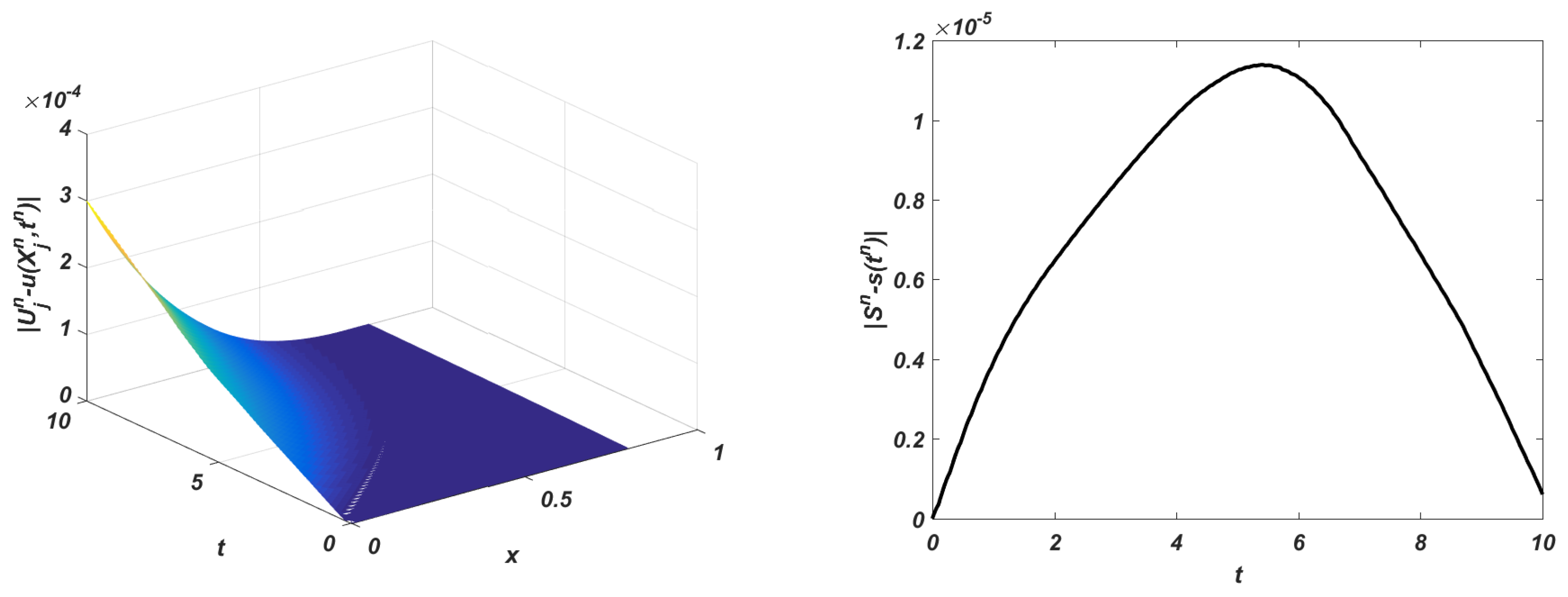
Note that the exact positions of the grid nodes, $x_j^n$, $0\le j\le J$, $0\le n\le N$, are unknown, so we compared them with the solution on the computed grid $X_j^n$, $0\le j\le J$, $0\le n\le N$. In Figure 1, we show the evolution of the computed error in both consumer and resource populations. We observe that the error is produced mainly at the birth (minimum size) and increases with time.

We can also obtain the experimental order of convergence by means of the following well-known formula:

$${\widehat{order}}_{2h,2k}=\frac{log({\widehat{e}}_{2h,2k}^{†}/{\widehat{e}}_{h,k}^{†})}{log2}.$$

We can show the convergence of our method and that it is second-order accurate by means of

Table 1. T = 10. For each value of h and k, the corresponding upper number is ${\widehat{e}}_{h,k}^{†}$; the lower number is ${\widehat{order}}_{h,k}^{†}$.

$\mathit{h}\backslash \mathit{k}$	1.25 × 10−2	6.25 × 10−3	3.125 × 10−3	1.5625 × 10−3	7.8125 × 10−4
1.25 × 10−1	3.003180 × 10−4	5.059363 × 10−5	9.929120 × 10−6	2.615432 × 10−5	2.965525 × 10−5
6.25 × 10−2	3.260311 × 10−4	7.522357 × 10−5	1.271462 × 10−5	2.473141 × 10−6	6.535886 × 10−6
		2.00	1.99	2.01	2.00
3.125 × 10−2	3.334010 × 10−4	8.200264 × 10−5	1.880835 × 10−5	3.186199 × 10−6	6.163402 × 10−7
		1.99	2.00	2.00	2.00
1.5625 × 10−2	3.359480 × 10−4	8.344165 × 10−5	2.046955 × 10−5	4.704060 × 10−6	7.979058 × 10−7
		2.00	2.00	2.00	2.00
7.8125 × 10−3	3.363417 × 10−4	8.380967 × 10−5	2.093071 × 10−5	5.118703 × 10−6	1.176429 × 10−6
		2.00	2.00	2.00	2.00

. In the test, the initial size interval was taken as $[0,x_M^0]$, with $x_M^0=0.8$, and the numerical integration was carried out on the time interval $[0,T]$, with $T=10$. Each column and each row of the table represent a computation with different values of the time and size discretization parameters, respectively. The upper number of each entry in columns two to six of said table represents the error computed from (64) and the lower quantity is the experimental order of convergence. We also remark that the ratio $r:=k/h$ was kept fixed as soon as we considered approximations along each diagonal of the table. We realize that the results in Table 1 clearly confirm the expected (theoretically) second-order convergence for these approximations. Different values of parameters $\rho$ and $\lambda$ confirm the same behavior of the error.

5. Conclusions

We proposed a numerical method specially adapted to integrate a model that describes the evolution of a size-structured consumer population feeding on a dynamical resource. The model couples a first-order hyperbolic partial differential equation with nonlocal and nonlinear boundary condition and a differential equation driving the dynamics of the resource. The novelty of the model is the appearance of a delay in the resource evolution rate. Numerical methods are the only feasible approach, except in exceptional cases, for the approximation of the solution of the problem and eventually studying the dynamical behavior of the model. The authors have in preparation [15], using this model, a numerical study on the effect of the delay in the resource evolution rate on the dynamics of a population of the Daphnia magna (water flea).

The analyzed numerical method integrated the problem along its characteristic curves. We proved optimal second-order of convergence to the solution; this was confirmed numerically by means of an academic test problem. This is the first convergence analysis to our knowledge for the discretization of this kind of problem.

References

Ruan, S. Delay differential equations in single species dynamics. In Delay Differential Equations and Applications; Arino, O., Hbid, M.L., Ait Dads, E., Eds.; Springer: Berlin, Germany, 2006; pp. 477–517. [Google Scholar]
Kooijman, S.A.L.M.; Metz, J.A.J. On the dynamics of chemically stressed populations: The deduction of population consequences from effects on individuals. Ecotoxicol. Environ. Saf.1984, 8, 254–274. [Google Scholar] [CrossRef]
Thieme, H.R. Well-posedness of physiologically structured population models for daphnia magna. J. Math. Biol.1988, 26, 299–317. [Google Scholar] [CrossRef][Green Version]
De Roos, A.M.; Metz, J.A.J.; Evers, E.; Leipoldt, A. A size dependent predator-prey interaction: Who pursues whom? J. Math. Biol.1990, 28, 609–643. [Google Scholar] [CrossRef]
Diekmann, O.; Gyllenberg, M.; Metz, J.A.J.; Nakaoka, S.; de Roos, A.M. Daphnia revisited: Local stability and bifurcation theory for physiologically structured population models explained by way of an example. J. Math. Biol.2010, 61, 277–318. [Google Scholar] [CrossRef] [PubMed]
De Roos, A.M.; Diekmann, O.; Getto, P.; Kirkilionis, M.A. Numerical equilibrium analysis for structured consumer resource models. Bull. Math. Biol.2010, 72, 259–297. [Google Scholar] [CrossRef] [PubMed]
Diekmann, O.; Getto, P.; Gyllenberg, M. Stability and bifurcation analysis of volterra functional equations in the light of suns and stars. SIAM J. Math. Anal.2007, 39, 1023–1069. [Google Scholar] [CrossRef][Green Version]
De Roos, A.M. Numerical methods for structured population models: The escalator boxcar train. Numer. Methods Partial. Differ. Equations1988, 4, 173–195. [Google Scholar] [CrossRef]
Angulo, O.; López-Marcos, J.C.; López-Marcos, M.A. Analysis of an efficient integrator for a size-structured population model with a dynamical resource. Comput. Math. Appl.2014, 68, 941–961. [Google Scholar] [CrossRef]
Brännström, Å.; Carlsson, L.; Simpson, D. On the convergence of the escalator boxcar train. SIAM J. Numer. Anal.2013, 51, 3213–3231. [Google Scholar] [CrossRef]
Carrillo, J.A.; Gwiazda, P.; Kropielnicka, K.; Marciniak-Czochra, A.K. The escalator boxcar train method for a system of age-structured equations in the space of measures. SIAM J. Numer. Anal.2019, 57, 1842–1874. [Google Scholar] [CrossRef]
Angulo, O.; López-Marcos, J.C. Numerical integration of fully nonlinear size-structured population models. Appl. Numer. Math.2004, 50, 291–327. [Google Scholar] [CrossRef]
Angulo, O.; López-Marcos, J.C. Numerical schemes for size-structured population equations. Math. Biosci.1999, 157, 169–188. [Google Scholar] [CrossRef]
López-Marcos, J.C.; Sanz-Serna, J.M. Stability and convergence in numerical analysis III: Linear investigation of nonlinear stability. IMA J. Numer. Anal.1988, 8, 71–84. [Google Scholar]
Abia, L.; Angulo, O.; López-Marcos, J.C.; López-Marcos, M.A. A numerical study on the effect of a delay in the resource evolution rate in the dynamics of a population of Daphnia magna. in preparation.
Figure 1.k = 1.25 × 10⁻², h = 1.25 × 10⁻¹.Plot on the left: evolution of the error in the consumer population; plot on the right: evolution of the error in the resource population.