Article

Study of Transition Zones in the Carbon Monoxide Catalytic Oxidation on Platinum Using the Network Simulation Method

1
Department of Applied Physics and Naval Technology, Universidad Politécnica de Cartagena (UPCT), Campus Alfonso XIII, 30202 Cartagena, Spain
2
Department of Mechanical Engineering, Materials and Manufacturing, Universidad Politécnica de Cartagena (UPCT), 30202 Cartagena, Spain
3
Metallurgical and Mining Engineering Department, Universidad Católica del Norte, Antofagasta 1240000, Chile
*
Author to whom correspondence should be addressed.
Mathematics 2020, 8(9), 1413; https://doi.org/10.3390/math8091413
Submission received: 29 July 2020 / Revised: 17 August 2020 / Accepted: 20 August 2020 / Published: 24 August 2020
(This article belongs to the Section Engineering Mathematics)

Abstract

:
A study of transition zones in the carbon monoxide catalytic oxidation over platinum is presented. After the design of a network model following the rules of the Network Simulation Method, it is run in a standard (free) software providing the fractional coverages of all species for different values of carbon monoxide partial pressure, the main parameter that produces the change between a stationary or periodic response. The design of the model is explained in detail and no assumptions are made concerning the removing of oxidation fractional coverage. The illusory chaotic behavior associated with an inadequate time step in the numerical algorithm is studied. This work provides an explanation for the transition (bifurcation) between the stationary and the periodical response studies making use of Poincaré plane and phase-diagrams. The extinction of variable fluctuation in the transition zone is analyzed to understand its relation with given values of transition partial pressures. Of particular interest is the small time span of the superficial fractional coverage of carbon monoxide fluctuation near the second transition partial pressure.

1. Introduction

The name “catalysis” was first used in 1836 by Berzelius for chemical reactions that involve the use of compounds, called catalysts, to accelerate these processes without being consumed [1]. A catalyst speeds up a reaction by lowering one or more activation energies or by introducing an alternative reaction with a lower activation energy; a catalyst should be selective. As a consequence, the activation energy for the desired product should be considerably diminished [2,3]. One of these processes, the catalytic oxidation of carbon monoxide on platinum, an example of air–metal interface oxidation with adsorption, is used in noble metal catalytic converters, which are common components in modern automobile engines. These systems are usually classified into two types: three-way and oxidation converters. However, from the point of view of the chemical reaction analysis, both are similar, a reason for which they are often considered the same type of chemical reaction.
A review of the literature reveals that there are four different approaches to modeling the chemical reactions that occur in these systems: the classical converter approach, the tanks-in-series approach, the more complex tanks-in-series approach and the Ford three-way converter model [4]. The classical converter approach first described by Oh and Cavendish [5] is based on a 1-D mass transfer model with chemical reactions and heat transfer. Chen et al. [6] extended this model to 3-D to study the effects of heat loss and to evaluate a series of design parameters. Katashiba et al. [7] used a zero-dimensional (tanks-in-series) approach, a model that was designed to comply with fuel control system optimization and so was simpler than the above. In this model, the new approach is to assume quasi-homogeneous reactions where the catalyst is divided into n elements to which global kinetics are applied with explicit velocity expressions. In addition, the capacity to store oxygen by the converter was also taken into account. Gottberg et al. [8] developed a more complex tanks-in-series approach, in an attempt to optimize potential exhaust after treatment technologies, a model that assumes a less sophisticated macromixing modelization of the flow applying an advanced treatment of the chemical kinetics modelization. This treatment is characterized by an independent calculation of the reactions and adsorption/desorption rates, but has the disadvantage of needing excessive computing times. Finally, Montreuil et al. [9] used a model designed for assuming Pt/Rh current generation and Pd/Rh catalysts in Ford vehicles for steady state operation, with the same specifications as the 1-D model mentioned above but incorporating a complicated system of 13 reactions.
The model in this work, proposed by Langmuir–Hinshelwood, simulates the carbon monoxide oxidation reaction over platinum. This mechanism has been used in many science and engineering problems, mainly in catalytic problems [10,11,12,13,14]. From experimental studies, this mechanism is developed in three steps, [15,16,17,18]: adsorption of carbon monoxide, dissociative chemisorbed oxygen and desorption of carbon dioxide. Some authors have added a slow step to the Langmuir–Hinshelwood mechanism: periodical oxidation-reduction on a catalytic surface [19,20]. Recently, L’vov and Galwey proposed a new mechanism for the catalytic oxidation of CO in platinum through an intermediate species in the platinum (IV) oxide, with two clearly differentiated kinetics: one for the oxidation of CO and the other for the restoration of the platinum oxide layer [21]. Most catalytic converters studied use simple explicit velocity expressions, despite the evidence of multiple isothermal steady state and auto-sustained oscillations [15]. Recent works have managed to measure the different rates of the active processes in the reaction for the oxidation of CO in platinum using molecular beams [22,23]. In addition, other works propose new methodologies and techniques that may be useful to measure the mentioned reaction rates based on a predictive approach [24].
The network model that implements the governing equation and boundary conditions of the problem, which has been designed following the rules of the network simulation method (Gonzalez-Fernandez and Alhama [25] and Sanchez-Perez et al. [26]), is run in the standard circuit simulation software NgSpice or PSpice [27,28,29]. This method has been widely used in a large variety of engineering problems such as corrosion, fluid flow, heat transfer, inverse problem, etc. [30,31,32,33,34,35].
The aims of this work are twofold. On the one hand, the design of a Network Model to simulate the catalytic oxidation in platinum of carbon monoxide. On the other hand, the investigation of the transition zones where the catalytic chemical reaction extinction occurs. This study is carried out through different phase diagrams and Poincaré planes. The results of the simulations are successfully compared with others coming from experiments.

2. Governing Equations

Figure 1 shows the three steps of the Langmuir–Hinshelwood mechanism, represented by the following chemical equations [17].
C O +   k 1 k 1 C O a d s
O 2 +   2 k 2 k 2 2 O a d s
C O a d s +   O a d s k r C O 2 +   2
where * represents the surface hole effects.
The kinetic equations associated with the above chemical equation are [17]:
d C C O d t = k 1 · C C O α 1 · C α 2 + k 1 · C C O a d s α 3
d C O d t = k 2 · C O β 1 · C β 2 + k 2 · C O a d s β 3
The following additional chemical equations are introduced to consider the nature of the platinum surface in the catalytic process:
C O a d s +   [ P t O a d s ] k r e d C O 2 +   2
P t + O a d s k o x [ P t O a d s ]
where [PtOads] represents oxidative species.
The respective kinetic equations associated with the above chemical equation are:
d C C O a d s d t = k r e d · C C O a d s δ 1 · C [ P t O a d s ] δ 2 k r · C C O a d s γ 1 · C O a d s γ 2 + k 1 · C C O α 1 · C α 2 k 1        · C C O a d s α 3
d C O a d s d t = k o x · C O a d s ω 1 · C P t ω 2 k r · C C O a d s γ 1 · C O a d s γ 2 + k 2 · C O β 1 · C β 2 k 2 · C O a d s β 3
Carbon monoxide molecules can be attached to any part of the platinum surface to prevent oxygen chemisorption. Assuming the hypothesis described by Keren and Sheintuch [18], oxygen chemisorption over platinum, usually a dissociative process, is produced by a molecular bond break in a vacancy of crystalline structure on the surface. Carbon dioxide desorption, though much faster than the processes described above, influences the suppression of the other species [18]. It is assumed that these reactions are isothermal and that the partial reactive pressures, Pj, remain constant [18].
The kinetic equations, which are written with fractional coverages, θ, (more suitable than species concentrations because they are directly related with partial pressure and the cover surface) and dimensionless superficial density, y, yield the following balance equations [17]:
d θ 1 d t o = A 1 ε o x ( 1 θ 1 θ 2 ) D 1 ε o x θ 1 1 ε o x y θ 1 θ 2 ( 1 y ) θ 1 θ 1 2 ( 1 y ) + θ 1 μ o x y θ 2
d θ 2 d t o = 2 A 2 ε o x y ( 1 θ 1 θ 2 ) 2 2 D 2 ε o x y θ 2 2 1 ε o x y θ 1 θ 2 μ o x y θ 2 θ 2 ( 1 y ) θ 1 + μ o x y θ 2 2
d y d t o = y ( 1 y ) θ 1 μ o x y 2 θ 2
where species j=1 refers to carbon monoxide and 2 to oxygen, y = X X T ,   A 1 = k 1 P 1 k r X T ,   A 2 = k 2 P 2 k r ,   D 1 = k 1 k r X T ,   D 2 = k 2 k r ,   μ o x = k o x k r e d ,   ε o x = k r e d k r .
In this equation the time, t, is divided by τsox, the characteristic time of Equation (6) and equal to 1/kred·XT. Thus, the variable t° is dimensionless. Now, εox can also be written as τrsox, where τr, the characteristic time of Equation (3), is equal to 1/kr·XT.
The fractional coverage of a species can be described as its superficial density, ns, and the ratio between activated surface and total surface. The superficial density, X, in turn, can be described as the subtraction between its maximum, XT, and the superficial ratio of catalyst blocked by the oxide.

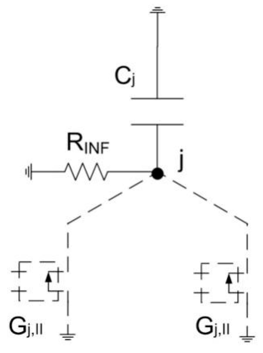
3. The Network Model

From Equations (10) to (12), three coupled networks are formed, one per variable, following the indications given by González-Fernández and Alhama, and Sanchez-Perez (González-Fernández and Alhama, 2001, Sanchez-Perez, 2012, Sanchez-Perez et al., 2018). However, to facilitate your understanding, the steps for its design will be briefly explained. First, the equivalence between variable and electric voltage must be established (θj (fractional coverage) ≡ V (electric voltage) and y (activated surface density) ≡ V).
Second, each sum of Equations (10) to (12) is considered an electric current, Ij, that balances at a central node (Figure 2). The time derivative of each variable, d θ j d t and d y d t , is implemented as a capacitor, Cj, and the rest of the addends as controlled current sources, Gj. So, the current Ij for variable j = 1, according to Equation (10), can be separated into two controlled current sources, I 1 , I = A 1 ε o x ( 1 θ 1 θ 2 ) ( G 1 , I ) ,     I 1 , I I = D 1 ε o x θ 1 ( G 1 , I I ) ,   I 1 , I I I = 1 ε o x y θ 1 θ 2 ( G 1 , I I I ) ,   I 1 , I V = ( 1 y ) θ 1 ( G 1 , I V ) ,   I 1 , V = ( 1 y ) θ 1 2 ( G 1 , V )   and I 1 , V I = θ 1 μ o x y θ 2 ( G 1 , V I ) with θ1, θ2 and y being the voltages at the central node of each variable’s network. The last term of the circuit (Figure 2) is a resistor, RInf, with supposedly infinite value to give stability to the circuit.
Thereby, for variables 1 and 2, the network model contains six controlled current sources and two for variable y (Figure 3).
Finally, the model can be simulated with a standard circuit simulation code such as NgSpice or Pspice [27,28,29].
The software NgSpice [29] makes use of the most powerful computational algorithms required for the circuit simulation software to afford strong non-lineal and coupled mathematical models such as that described in this paper. These algorithms, based on the thesis of Nagel [36] and described in the NgSpice’s manual [37], include trapezoidal integration [27], Gear´s fixed time methods [38] and the Runge–Kutta algorithm. The accuracy and efficiency of these methods are provided by reducing the local truncation error and the stability in the convergence of the numerical solution.

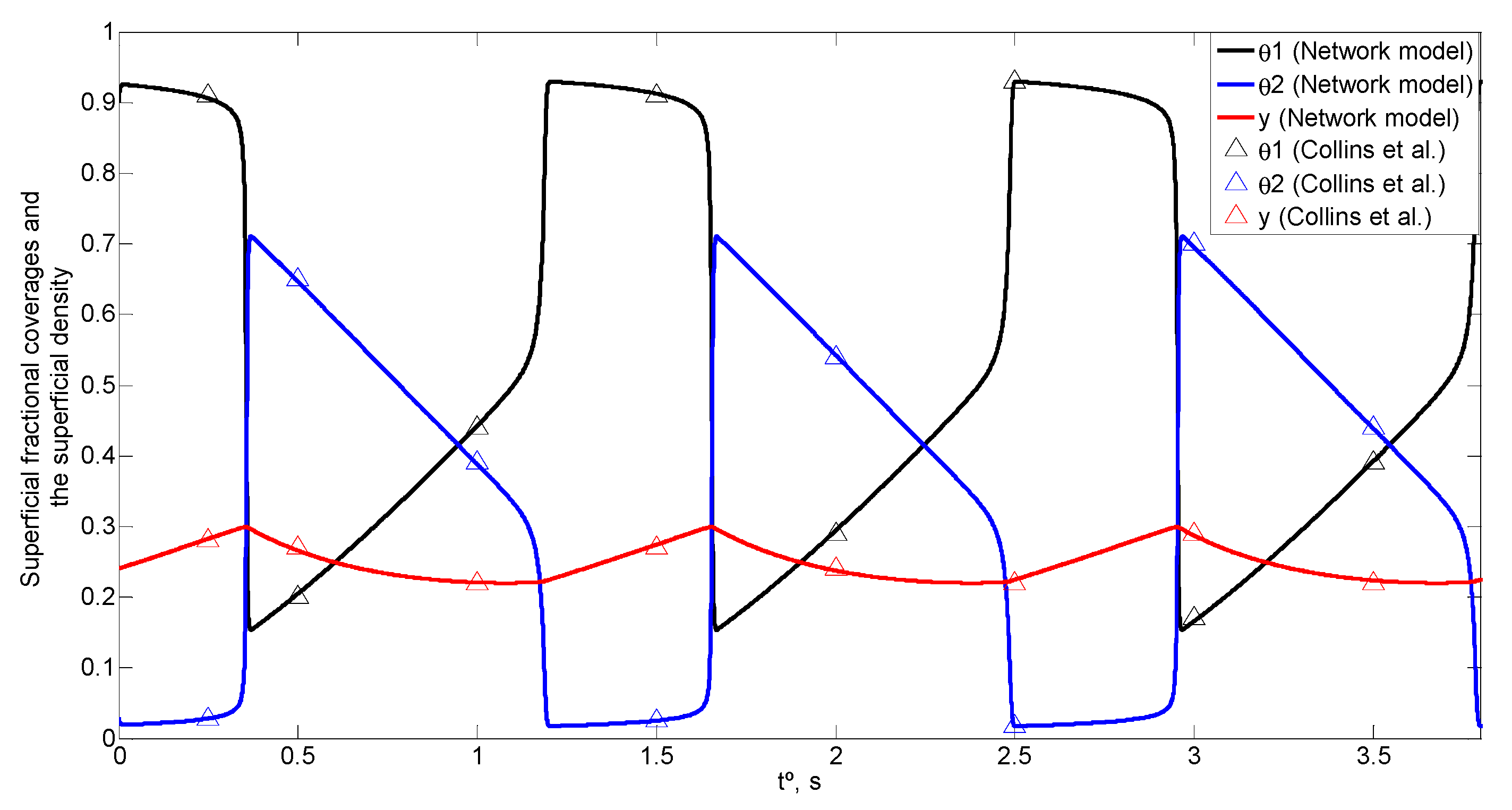
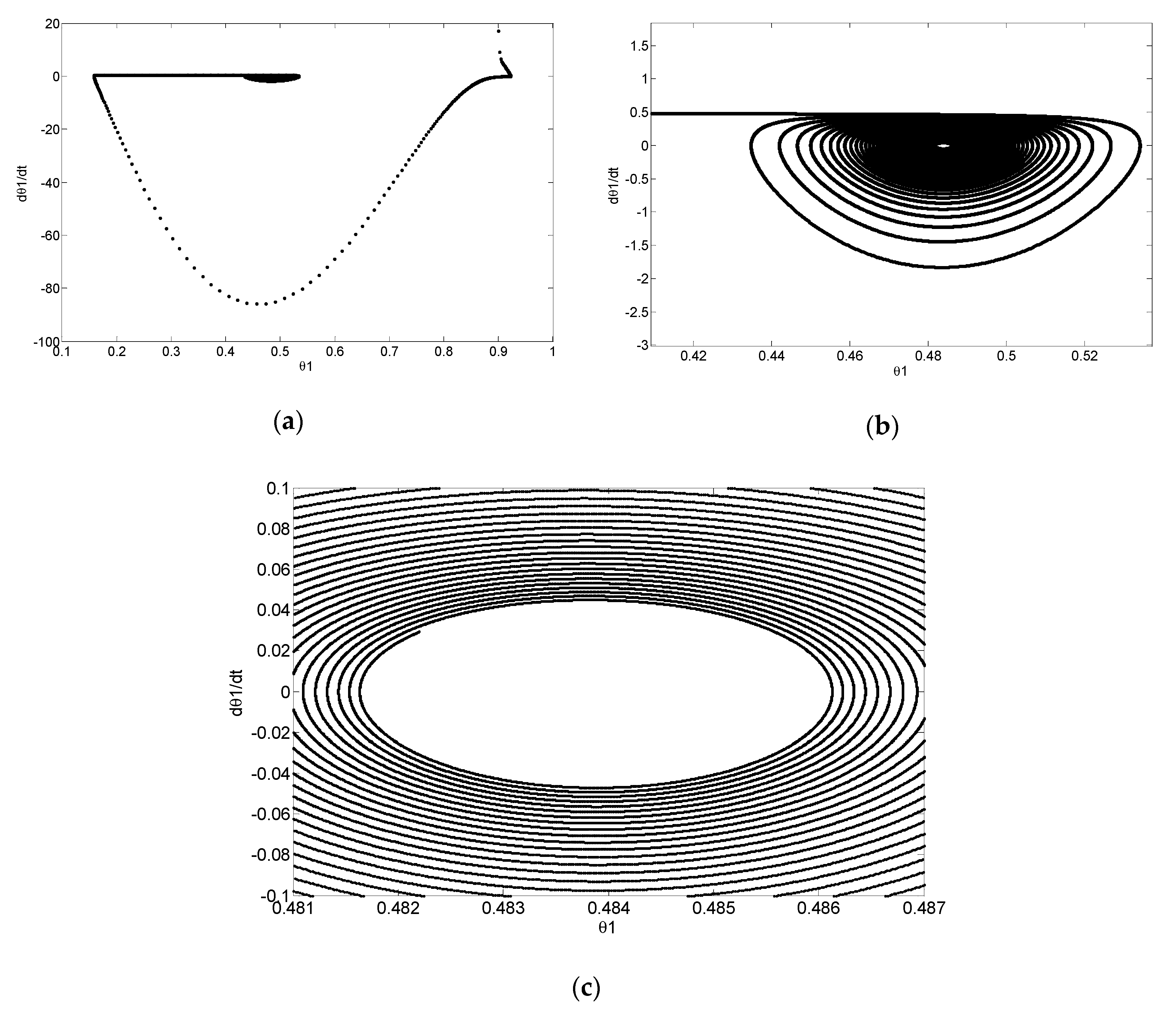
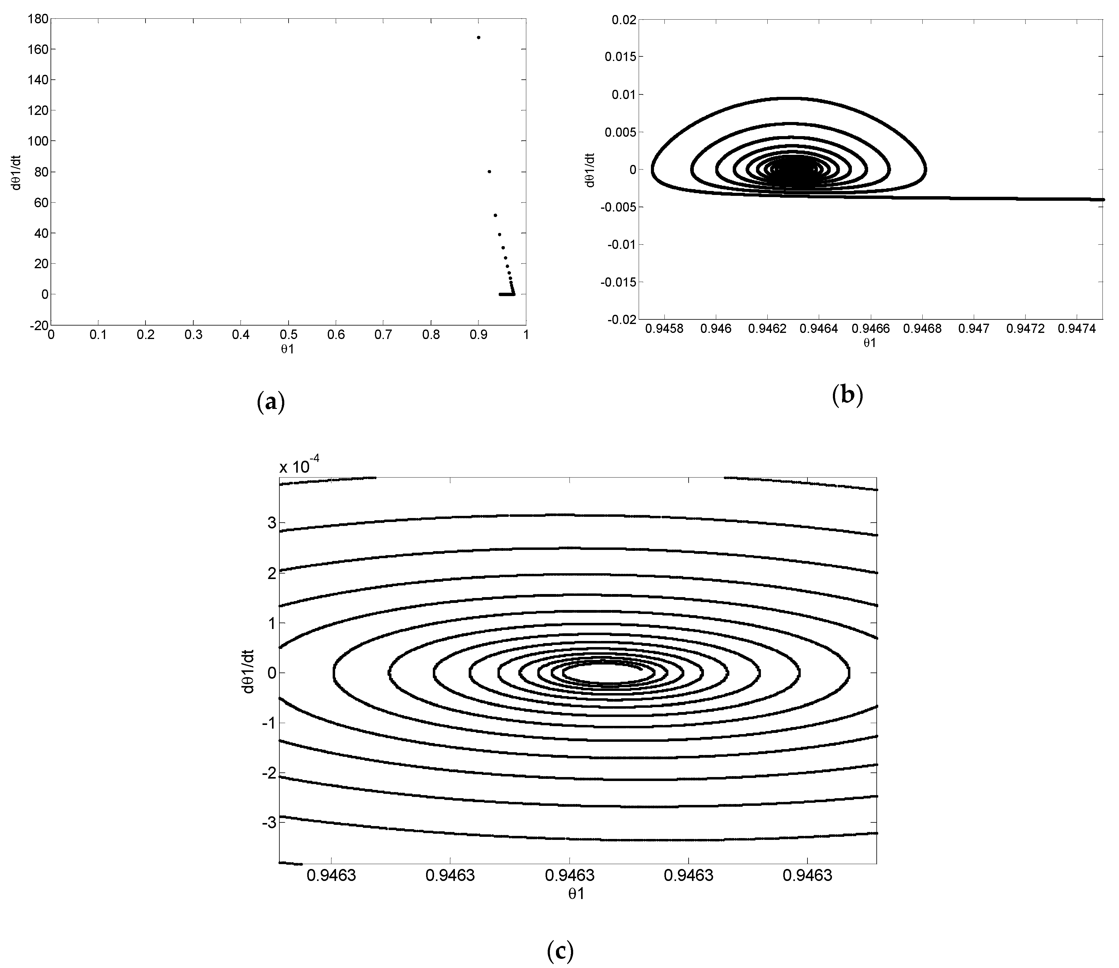
4. Simulation and Results

The first data used to characterize the reactions are the activation energies. The values of the dimensionless kinetic constants, D1, D2, μox and εox are 0.01, 0.0005, 5 and 0.0001, respectively. Other dimensionless constants used in Equations (10) and (11) are A1 and A2, with values 0.002475·P1 and 3, respectively [17].
To verify the model, we used the carbon monoxide partial pressure variable, P1, from several former experimental and numerical studies, 101.324 Pa [17,19,39,40,41,42]. In the same way, the initial conditions for θ1, θ2 and y (0.9, 0.03 and 0.24, respectively) are applied.
Figure 4 shows the periodic fluctuation of superficial fractional coverages and superficial density, which is similar to the results described in the above mentioned studies.
Figure 5, Figure 6 and Figure 7 show the amplitude values of superficial fractional coverages and the superficial density far from the initial time as a function of carbon monoxide partial pressure. This parameter strongly influences the reactions as a result of its relation with the carbon monoxide concentration. In the same figures, it is possible to distinguish three zones: these transitions are partially mentioned by Collins et al., Keren and Sheintuch and Carlsson et al. [17,18,43].
Following the indication given by Sanchez-Perez [44], in the first zone, up to 99.992 Pa, the studied variables have stationary values, that is, the converter is not operative. Within this zone, the value of superficial fractional coverage of carbon monoxide increases as its partial pressure increases (Figure 5) which is the opposite to the behaviour of the superficial fractional coverage of oxygen (Figure 6). Obviously, the number of carbon monoxide molecules inside the gas phase depends on its partial pressure, and the surface they occupy on the converter follows the same relation. For this reason, the superficial fractional coverage increases as the partial pressure increases. The superficial fractional coverage of oxygen depends on the behaviour of the carbon monoxide. This reasoning is also valid for the superficial density, Figure 7.
In the second zone, from 99.992 to 186.651 Pa, the studied variables fluctuate, that is, the converter is operative. Of note is the relation between the superficial fractional coverages of oxygen and carbon monoxide, θO/θCO, that is, nOs/nCOs is 0.36/0.48. This is the same as the inverse relation between oxygen and carbon atomic weights, 3/4. Therefore, there is a relation between the volume ratio of the two species and the respective surface they occupy, when fluctuation starts. The explanation lies in the optimal distribution of atoms on the converter surface, considering that the carbon monoxide molecule, before binding with the second oxygen atom, adheres to the surface through the carbon atom. Fluctuation increases its amplitude as the carbon monoxide partial pressure increases. Finally, the amplitude reaches a level that stops the fluctuation. In the third zone, above 186.651 Pa, the studied variables become stationary, that is, the converter is not operative.
To understand the superficial fractional coverages and the superficial density behaviour inside the first zone, we choose a partial pressure belong to this zone, 39.997 Pa. Figure 8 shows the evolution of these variables; note that the variables tend asymptotically towards a constant value. As the carbon monoxide partial pressure approaches the transition value between the first and the second zone, the superficial fractional coverages and the superficial density start to fluctuate, Figure 9.
The closer to the second zone, the greater the time needed for the process to stop (Figure 9d). Figure 10 shows the phase diagram, in which it is possible to distinguish the slow annihilation rate. Note that a very small time step is needed in the numerical algorithm, 10−4 s, compared with the total time of several seconds, to attain sufficient accuracy. An unsuitable selection of the time step depicts an incorrect solution, such as chaotic behaviour.
The same study was made for the second zone. As shown in Figure 4, for a partial pressure of 101.324 Pa inside this zone, the variables fluctuate periodically. Figure 11a shows the periodical fluctuation close to the transition zone between the second and the third zones. Of note is the small span elapsed as superficial fractional coverage of carbon monoxide values change. As the carbon monoxide partial pressure approaches the transition value between the second and the third zone, the superficial fractional coverages and the superficial density stop fluctuating, Figure 11b.
Figure 12 shows the phase diagram, in which it is possible to distinguish the slow annihilation rate. Note that only a very small time step in the numerical algorithm is necessary for sufficient accuracy; hence, an unsuitable selection of the time step depicts an incorrect solution, such as chaotic behaviour.
The comments concerning the first zone are applicable to the third zone, Figure 13.
Figure 14 shows a more detailed study, using a phase plane, of the superficial fractional coverage of carbon monoxide at its partial pressure of 140 Pa (second zone), which is clearly periodical. Figure 15, a phase space, represents a detail of the change of superficial fractional coverage on its right side. Once again, the short time step used in the numerical algorithm necessary to obtain a clear image is of note, as is used in the later figures. The single point in Figure 16, a Poincaré plane for its period (1.599 s), confirms the periodicity of the superficial fractional coverage fluctuation of carbon monoxide.
A comparison of Figure 10 and Figure 14 reveals a similar pattern at different scales. Note that the low velocity section is interrupted in Figure 10.
We now analyse the boundary between zones. Figure 17 shows the relation between superficial fractional coverage of carbon monoxide and the superficial density for a carbon monoxide pressure belonging to the first zone close to the transition to the second zone. The initial conditions have been changed to depict the fact that these values have no influence. The explanation of this transition clearly involves an equilibrium point in the dynamical system, and a similar explanation is applicable to the transition between the second and third zones.

5. Conclusions

A clear insight into the catalytic converter function, especially as regards the different zones of carbon monoxide partial pressure, is gained by means of the proposed model in this paper whose design is based on the Network Simulation Method. The model assumes no simplifications in the governing equations and is run in a standard circuit simulation software with negligible computing time. The incorrect selection of the time step in the numerical simulation has a remarkable influence on the results, introducing an illusory chaotic behaviour when it is not small enough.
The simulations of the model also provide an explanation for the transition between the stationary and the periodical response, an issue that is partially discussed by other authors. Each transition zone, a bifurcation, brings up an additional numerical difficulty in the selection of the parameters of the computing solver and demands a special understanding of the numerical tool to avoid misapplications that give rise to a limit cycle instead of chaotic behaviour and the opposite. In addition, the start and extinction of the fluctuations, which are also relevant from the point of view of the technical control of the catalysis, are analysed to understand their relation with the carbon monoxide partial pressures, the control parameter of the system.
The methodology applied to the study of this chemical process, based on the use of the Poincaré plane and phase-diagrams, is suitable in the analysis of chaotic systems. Despite the difficulty of choosing the location (or the characteristic time) for the Poincaré plane, this analytical tool is quite effective since it reveals the nature of the system. The numerical simulations are successfully compared with experimental results from the literature.
It is worth mentioning the small time span in which the variables fluctuate near the extinction bifurcation, where the system stops working. The aforementioned two features, the time step and time span, introduced in this work are not mentioned in the available literature, which makes it possible to avoid the illusory chaotic behaviour.

Author Contributions

J.F.S.-P. came up with the initial idea for the work. J.F.S.-P. and J.A.M.N. performed the simulations and conceptualization. J.F.S.-P., J.A.M.N., F.A. and M.C. analyzed the data, made the formal analysis and participated in the writing and revising of the manuscript. J.F.S.-P., J.A.M.N., F.A. and M.C. have read and agreed to the published version of the manuscript.

Funding

This research received no external funding.

Conflicts of Interest

The authors declare no conflict of interest.

References

  1. Sinfelt, J.H. Role of surface science in catalysis. Surf. Sci. 2002, 500, 923–946. [Google Scholar] [CrossRef]
  2. Kolasinski, K.W. Surface Science: Foundations of Catalysis and Nanoscience; Wiley: Hoboken, NJ, USA, 2012; ISBN 9781119990369. [Google Scholar]
  3. Hendriksen, B.L.M.; Bobaru, S.C.; Frenken, J.W.M. Bistability and oscillations in CO oxidation studied with scanning tunnelling microscopy inside a reactor. Catal. Today 2005, 105, 234–243. [Google Scholar] [CrossRef]
  4. Pattas, K.N.; Stamatelos, A.M.; Pistikopoulos, P.K.; Koltsakis, G.C.; Konstandinidis, P.A.; Volpi, E.; Leveroni, E. Transient modeling of 3-way catalytic converters. In Proceedings of the SAE Technical Papers, Detroit, MI, USA, 1 March 1994. [Google Scholar]
  5. Oh, S.H.; Cavendish, J.C. Transients of Monolithic Catalytic Converters: Response to Step Changes in Feedstream Temperature as Related to Controlling Automobile Emissions. Ind. Eng. Chem. Prod. Res. Dev. 1982, 21, 29–37. [Google Scholar] [CrossRef]
  6. Chen, D.K.S.; Bissett, E.J.; Oh, S.H.; Van Ostrom, D.L. A three-dimensional model for the analysis of transient thermal and conversion characteristics of monolithic catalytic converters. In Proceedings of the SAE Technical Papers, Detroit, MI, USA, 1 February 1988; pp. 177–189. [Google Scholar]
  7. Katashiba, H.; Nishida, M.; Washino, S.; Takahashi, A.; Hashimoto, T.; Miyake, M. Fuel injection control systems that improve three way catalyst conversion efficiency. In Proceedings of the SAE Technical Papers, Detroit, MI, USA, 1 January 1991; pp. 196–204. [Google Scholar]
  8. Gottberg, I.; Rydquist, J.E.; Backlund, O.; Wallman, S.; Maus, W.; Brück, R.; Swars, H. New potential exhaust gas aftertreatment technologies for “clean Car” legislation. In Proceedings of the SAE Technical Papers, Detroit, MI, USA, 1 January 1991; pp. 343–360. [Google Scholar]
  9. Montreuil, C.N.; Williams, S.C.; Adamczyk, A.A. Modeling current generation catalytic converters: Laboratory experiments and kinetic parameter optimization-steady state kinetics. In Proceedings of the SAE Technical Papers, Detroit, MI, USA, 1 February 1992. [Google Scholar]
  10. Messerer, A.; Niessner, R.; Pöschl, U. Comprehensive kinetic characterization of the oxidation and gasification of model and real diesel soot by nitrogen oxides and oxygen under engine exhaust conditions: Measurement, Langmuir-Hinshelwood, and Arrhenius parameters. Carbon N. Y. 2006, 44, 307–324. [Google Scholar] [CrossRef]
  11. Vasanth Kumar, K.; Porkodi, K.; Selvaganapathi, A. Constrain in solving Langmuir-Hinshelwood kinetic expression for the photocatalytic degradation of Auramine O aqueous solutions by ZnO catalyst. Dye. Pigment. 2007, 75, 246–249. [Google Scholar] [CrossRef]
  12. Kumar, K.V.; Porkodi, K.; Rocha, F. Langmuir-Hinshelwood kinetics—A theoretical study. Catal. Commun. 2008, 9, 82–84. [Google Scholar] [CrossRef]
  13. Xu, W.; Kong, J.S.; Chen, P. Single-molecule kinetic theory of heterogeneous and enzyme catalysis. J. Phys. Chem. C 2009, 119, 2393–2404. [Google Scholar] [CrossRef]
  14. Khezrianjoo, S.; Revanasiddappa, H.D. Langmuir-Hinshelwood Kinetic Expression for the Photocatalytic Degradation of Metanil Yellow Aqueous Solutions by ZnO Catalyst. Chem. Sci. J. 2012. [Google Scholar] [CrossRef]
  15. Burrows, V.A.; Sundaresan, S.; Chabal, Y.J.; Christman, S.B. Studies on self-sustained reaction-rate oscillations: I. Real-time surface infrared measurements during oscillatory oxidation of carbon monoxide on platinum. Surf. Sci. 1985, 160, 122–138. [Google Scholar] [CrossRef]
  16. Burrows, V.A.; Sundaresan, S.; Chabal, Y.J.; Christman, S.B. Studies on self-sustained reaction-rate oscillations II. The role of carbon and oxides in the oscillatory oxidation of carbon monoxide on platinum. Surf. Sci. Lett. 1987, 180, 110–135. [Google Scholar] [CrossRef]
  17. Collins, N.A.; Sundaresan, S.; Chabal, Y.J. Studies on self-sustained reaction-rate oscillations. III. The carbon model. Surf. Sci. 1987, 180, 136–152. [Google Scholar] [CrossRef]
  18. Keren, I.; Sheintuch, M. Modeling and analysis of spatiotemporal oscillatory patterns during CO oxidation in the catalytic converter. Chem. Eng. Sci. 2000, 55, 1461–1475. [Google Scholar] [CrossRef]
  19. Turner, J.E.; Sales, B.C.; Maple, M.B. Oscillatory oxidation of Co over a Pt catalyst. Surf. Sci. 1981, 103, 54–74. [Google Scholar] [CrossRef]
  20. Sales, B.C.; Turner, J.E.; Maple, M.B. Oscillatory oxidation of CO over Pt, Pd and Ir catalysts: Theory. Surf. Sci. 1982, 114, 381–394. [Google Scholar] [CrossRef]
  21. L’vov, B.V.; Galwey, A.K. Catalytic oxidation of CO on platinum. J. Therm. Anal. Calorim. 2013, 111, 145–154. [Google Scholar] [CrossRef]
  22. Neugebohren, J.; Borodin, D.; Hahn, H.W.; Altschäffel, J.; Kandratsenka, A.; Auerbach, D.J.; Campbell, C.T.; Schwarzer, D.; Harding, D.J.; Wodtke, A.M.; et al. Velocity-resolved kinetics of site-specific carbon monoxide oxidation on platinum surfaces. Nature 2018, 558, 280–283. [Google Scholar] [CrossRef]
  23. Harding, D.J.; Neugebohren, J.; Auerbach, D.J.; Kitsopoulos, T.N.; Wodtke, A.M. Using Ion Imaging to Measure Velocity Distributions in Surface Scattering Experiments. J. Phys. Chem. A 2015, 119, 12255–12262. [Google Scholar] [CrossRef]
  24. Rodger, J.A. Advances in multisensor information fusion: A Markov–Kalman viscosity fuzzy statistical predictor for analysis of oxygen flow, diffusion, speed, temperature, and time metrics in CPAP. Expert Syst. 2018, 35, e12270. [Google Scholar] [CrossRef]
  25. González-Fernández, C.F.; Alhama, F. Heat Transfer and the Network Simulation Method; Horno, J., Ed.; Transworld Research Network: Trivandrum, India, 2001. [Google Scholar]
  26. Sánchez-Pérez, J.F.; Marín, F.; Morales, J.L.; Cánovas, M.; Alhama, F. Modeling and simulation of different and representative engineering problems using network simulation method. PLoS ONE 2018, 13, e0193828. [Google Scholar] [CrossRef] [Green Version]
  27. Nagel, L.W.; Pederson, D.O. SPICE (Simulation Program with Integrated Circuit Emphasis); EECS Department: Berkeley, CA, USA, 1973. [Google Scholar]
  28. PSPICE 6.0; MicroSim Corporation Fairbanks: Irvine, CA, USA, 1994; Available online: http://robustdesignconcepts.com/files/pspice/index.htm (accessed on 15 January 2020).
  29. Sourceforge. NgSpice. Available online: http://ngspice.sourceforge.net/index.html (accessed on 15 January 2020).
  30. Horno, J.; González-Fernández, C.F.; Hayas, A. The network method for solutions of oscillating reaction-diffusion systems. J. Comput. Phys. 1995, 118, 310–319. [Google Scholar] [CrossRef]
  31. González Fernández, C.F.; Alhama, F.; López Sánchez, J.F.; Horno, J. Application of the network method to heat conduction processes with polynomial and potential-exponentially varying thermal properties. Numer. Heat Transf. Part. A Appl. 1998, 33, 549–559. [Google Scholar] [CrossRef]
  32. Zueco, J.; Alhama, F. Inverse estimation of temperature dependent emissivity of solid metals. J. Quant. Spectrosc. Radiat. Transf. 2006, 101, 73–86. [Google Scholar] [CrossRef]
  33. Sánchez, J.F.; Alhama, F.; Moreno, J.A. An efficient and reliable model based on network method to simulate CO2 corrosion with protective iron carbonate films. Comput. Chem. Eng. 2012, 39, 57–64. [Google Scholar] [CrossRef]
  34. Sánchez Pérez, J.F.; Moreno, J.A.; Alhama, F. Numerical Simulation of High-Temperature Oxidation of Lubricants Using the Network Method. Chem. Eng. Commun. 2015, 202, 982–991. [Google Scholar] [CrossRef]
  35. Sánchez-Pérez, J.F.; Alhama, F.; Moreno, J.A.; Cánovas, M. Study of main parameters affecting pitting corrosion in a basic medium using the network method. Results Phys. 2019, 12, 1015–1025. [Google Scholar] [CrossRef]
  36. Nagel, L.W. SPICE2: A Computer Program To Simulate Semiconductor Circuits. Ph.D. Thesis, University of California, Berkeley, CA, USA, 1975. [Google Scholar]
  37. Vogt, H.; Marcel, H.; Paolo, N. Ngspice User’s Manual Version 32; Sourceforge: San Diego, CA, USA, 2020; Available online: http://ngspice.sourceforge.net/index.html (accessed on 20 July 2020).
  38. Gear, C.W. The Automatic Integration of Ordinary Differential Equations. Commun. ACM 1971, 14, 176–179. [Google Scholar] [CrossRef]
  39. Beusch, H.; Fieguth, P.; Wicke, E. Thermisch und kinetisch verursachte Instabilitäten im Reaktionsverhalten einzelner Katalysatorkörner. Chem. Ing. Tech. 1972, 44, 445–451. [Google Scholar] [CrossRef]
  40. Lintz, H.-G.; Weisker, T. The oxidation of carbon monoxide on polycrystalline rhodium under knudsen conditions. Appl. Surf. Sci. 1985, 14, 251–258. [Google Scholar] [CrossRef]
  41. Lobban, L.; Luss, D. Spatial temperature oscillations during hydrogen oxidation on a nickel foil. J. Phys. Chem. 1989, 93, 6530–6533. [Google Scholar] [CrossRef]
  42. Tsai, P.K.; Wu, M.G.; Brian Maple, M. Oscillatory oxidation of CO over Pt at pressures from 10 to 760 torr. J. Catal. 1991, 127, 512–523. [Google Scholar] [CrossRef]
  43. Carlsson, P.A.; Zhdanov, V.P.; Kasemo, B. Bistable mean-field kinetics of CO oxidation on Pt with oxide formation. Appl. Surf. Sci. 2005, 239, 424–431. [Google Scholar] [CrossRef]
  44. Sánchez-Perez, J.F. Solución Numérica de Problemas de Oxidación Mediante el Método de Simulación por Redes. Ph.D. Thesis, Universidad Politécnica de Cartagena, Cartagena, Spain, 2012. [Google Scholar]
Figure 1. Essential mechanism of CO2 formation.
Mathematics 08 01413 g001
Figure 2. Scheme of the basic network model
Mathematics 08 01413 g002
Figure 3. Network model: (a) variable 1, (b) variable 2 and (c) variable y.
Mathematics 08 01413 g003
Figure 4. Evolution of superficial fractional coverages and the superficial density, P1 = 101.324 Pa.
Mathematics 08 01413 g004
Figure 5. Amplitude values at stationary superficial fractional coverage of carbon monoxide versus carbon monoxide partial pressure [44].
Mathematics 08 01413 g005
Figure 6. Amplitude values at stationary oxygen superficial fractional coverage versus carbon monoxide partial pressure [44].
Mathematics 08 01413 g006
Figure 7. Amplitude values at stationary superficial density versus carbon monoxide partial pressure [44].
Mathematics 08 01413 g007
Figure 8. Superficial fractional coverages and the superficial density evolution at P1 = 39.997 Pa [44].
Mathematics 08 01413 g008
Figure 9. Superficial fractional coverage of carbon monoxide evolution with time step = 2·10−4 s and at P1: (a) 94.6572 Pa, (b) 97.3236 Pa, (c) 98.6568 Pa and (d) 99.992 Pa.
Mathematics 08 01413 g009
Figure 10. Superficial fractional coverage of carbon monoxide phase plane at 99.992 Pa and time step = 2·10−4 s. (a) without zoom, (b) zoom on the spiral and (c) more precise zoom on the spiral.
Mathematics 08 01413 g010
Figure 11. Superficial fractional coverage of carbon monoxide evolution at time step = 2·10−4 s and P1: (a) 186.651 Pa and (b) 187.115 Pa.
Mathematics 08 01413 g011
Figure 12. Superficial fractional coverage of carbon monoxide phase plane at 187.115 Pa and time step = 2·10−4 s. (a) without zoom, (b) zoom on the spiral and (c) more precise zoom on the spiral.
Mathematics 08 01413 g012
Figure 13. Superficial fractional coverages and the superficial density evolution at P1 = 213.315 Pa [44].
Mathematics 08 01413 g013
Figure 14. Phase plane of superficial fractional coverage of carbon monoxide at P1 = 140 Pa and time step = 10−4 s.
Mathematics 08 01413 g014
Figure 15. Phase space of carbon monoxide superficial fractional coverage at P1 = 140 Pa and time step = 10−4 s.
Mathematics 08 01413 g015
Figure 16. Poincaré plane of superficial fractional coverage of carbon monoxide at P1 = 140 Pa and a period of 1.599 s.
Mathematics 08 01413 g016
Figure 17. Superficial fractional coverage of carbon monoxide versus superficial density at 99.992 Pa, with θ1 = 0.72525, θ2 = 0.52275 and y = 0.32595, and time step = 2·10−4 s. (a) without zoom, (b) zoom on the spiral.
Mathematics 08 01413 g017

