1. Introduction
In this paper, we review the unconditionally gradient stable Fourier-spectral method for several phase-field equations. The phase-field models are derived from the variational approach that minimizes the free energy of the system. Thus, the derived system follows a law of energy dissipation, which configures thermodynamic consistency, and hence leads to a mathematically well-posed model. The spectral methods, which belong to the collection of weighted residual methods, are originally derived to solve the spatial part of partial differential equations. For detailed, rigorous, and numerical aspect information on spectral methods, see [
1,
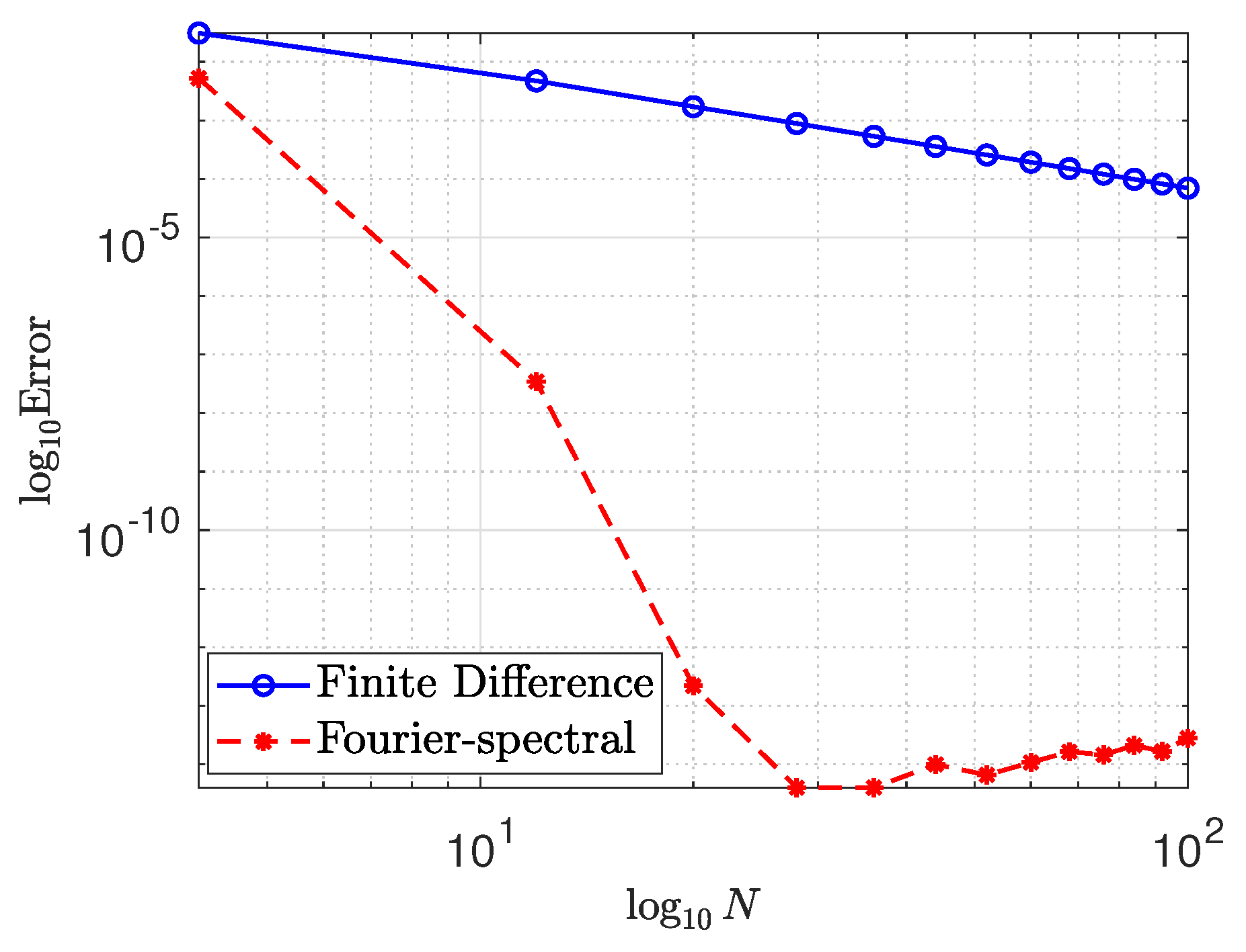
2] and the references therein. In spectral methods, one usually takes a finite set of the expansion functions (so called trial or basis functions) to represent the numerical solution as a linear combination of those functions. Choosing the expansion parts is important because they form a basis for entire spectral domain. Furthermore, we implicitly assume that those functions are smooth, therefore the most common choices are orthogonal polynomials and trigonometric functions. Since our focus is the Fourier-spectral method, the trigonometric basis functions are regarded as the trial functions. Moreover, instead of regarding entire continuous space, the representation is imposed only at discrete points; this is why this method is so called pseudo-spectral method. It is enable to one can save the computing resources in evaluating differentiation and employ the efficient algorithm such as the fast Fourier transform when the number of grid points is even. In addition, the error is decreasing exponentially when one employs the Fourier-spectral method while the finite difference methods lead to the algebraically decreasing order in fact.
Figure 1 shows the order of spectral accuracy compared with the order of accuracy of finite difference. In this case, we use a simple function
; hence
. An error is defined as
where
is an approximation of
.
According to
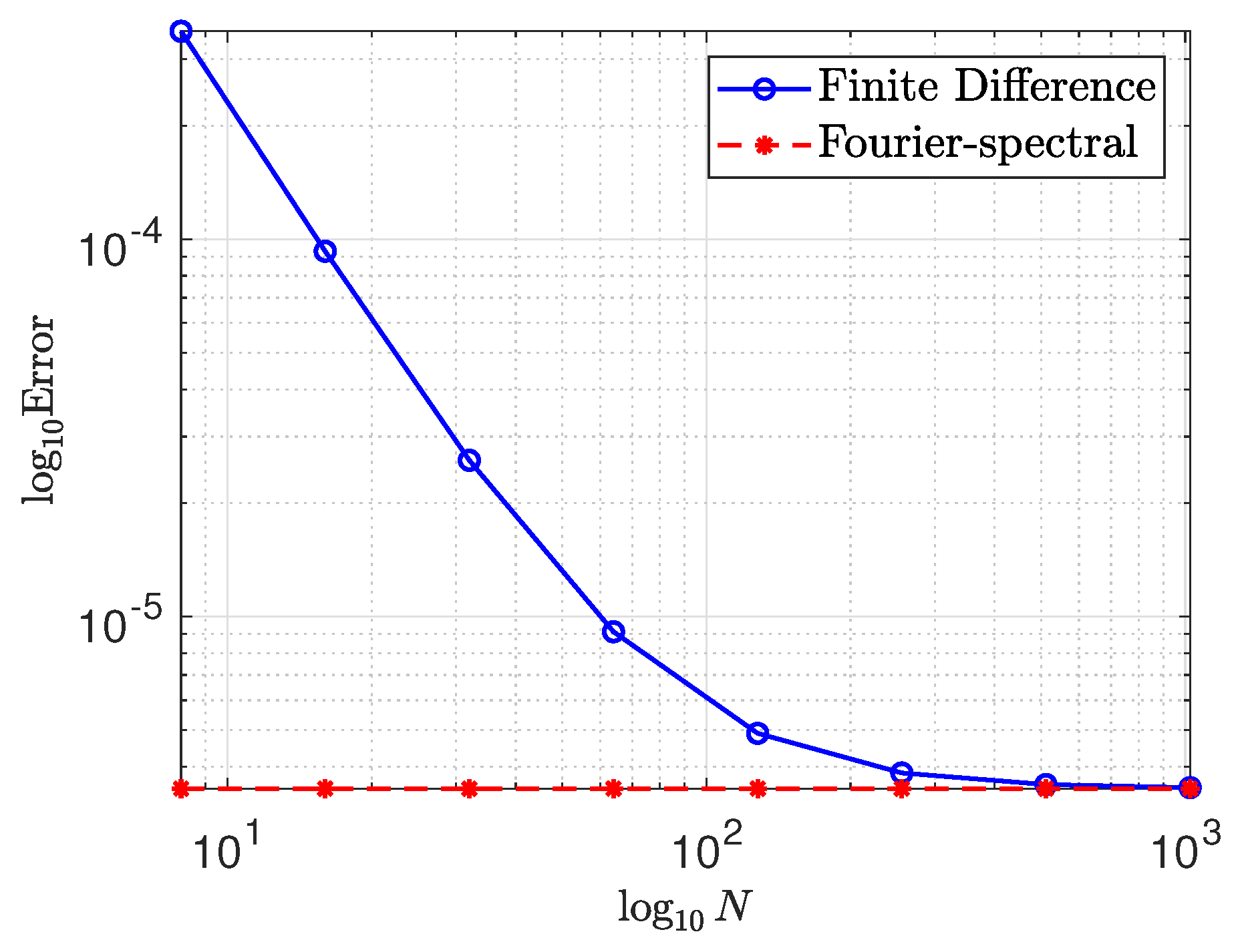
Figure 1, the error is decreasing exponentially via Fourier-spectral method indeed. Furthermore, we verify the efficiency of the Fourier-spectral method employing the following initial-boundary value problem in one-dimensional space with the
-periodic boundary condition.
Then, the exact solution of Equation (
1) is
. Define
as a numerical approximation to
for
where
is a time step and
is the number of iterations.
Figure 2 depicts the convergence of second-order central finite difference scheme and Fourier-spectral method. Note that the backward difference method in time is employed to both cases and an error is defined as
where
N is the number of grid points, hence the number of modes, and it is easily verified that the Fourier-spectral method requires relatively few grid points within similar accuracy indeed.
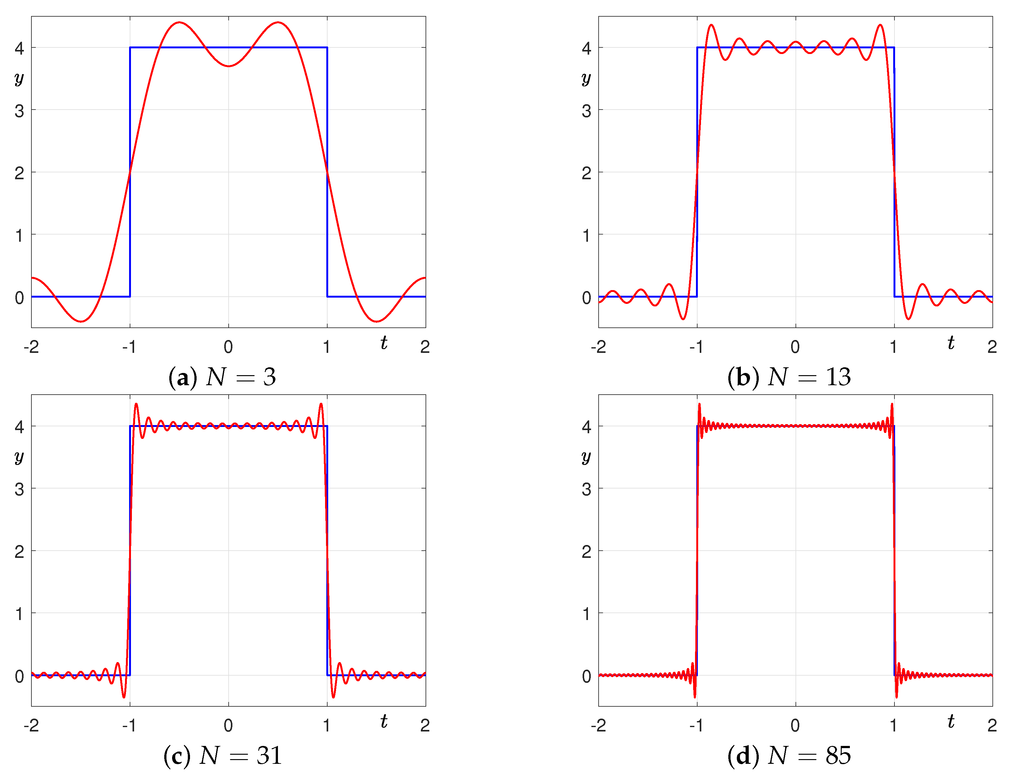
Sometimes, an interpolant cannot apply to less flexible domains since the method employs implicitly periodic or homogeneous boundary conditions though there is an advantage in numerical accuracy. Therefore, a somewhat subtle additional process is required to employ complex or mixed boundary conditions. Moreover, it causes Gibbs phenomenon if there is a point of discontinuity, i.e., when it has a sharp gradient.
Figure 3 shows the oscillations near discontinuities when one employs the Fourier interpolant.
Moreover, we set all the mobility terms in phase-field models as constant for convenience, more precisely set to 1 without loss of generality, since it requires further manipulation to handle a variable mobility in spectral methods [
3].
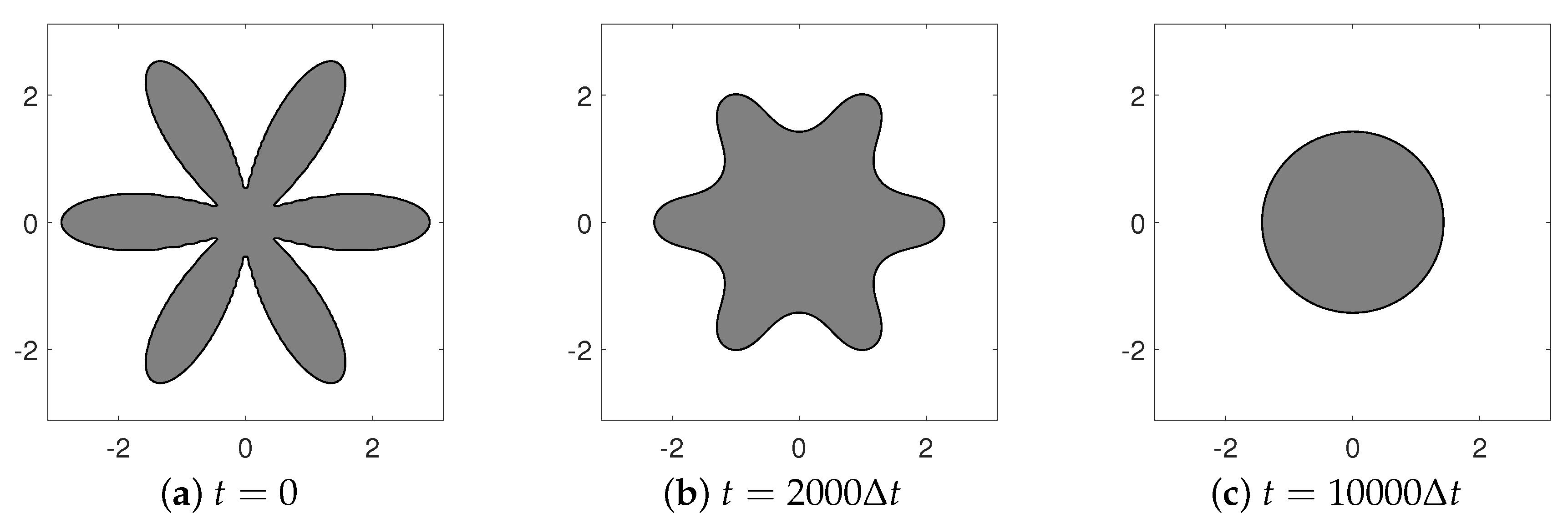
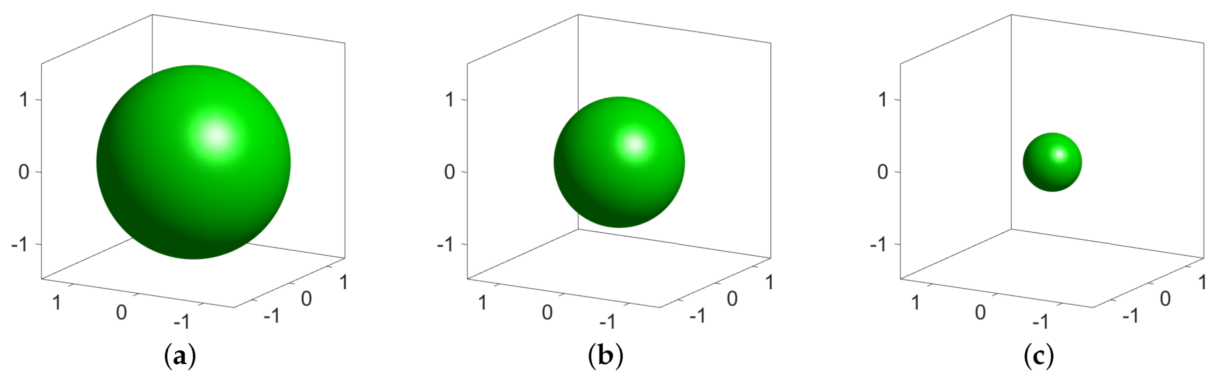
The Allen–Cahn (AC) equation is discussed first. It describes the temporal evolution of a non-conserved order field during anti-phase domain coarsening [
4]:
where
is defined as the difference between the concentrations of the two components in a mixture, which varies on
to 1,
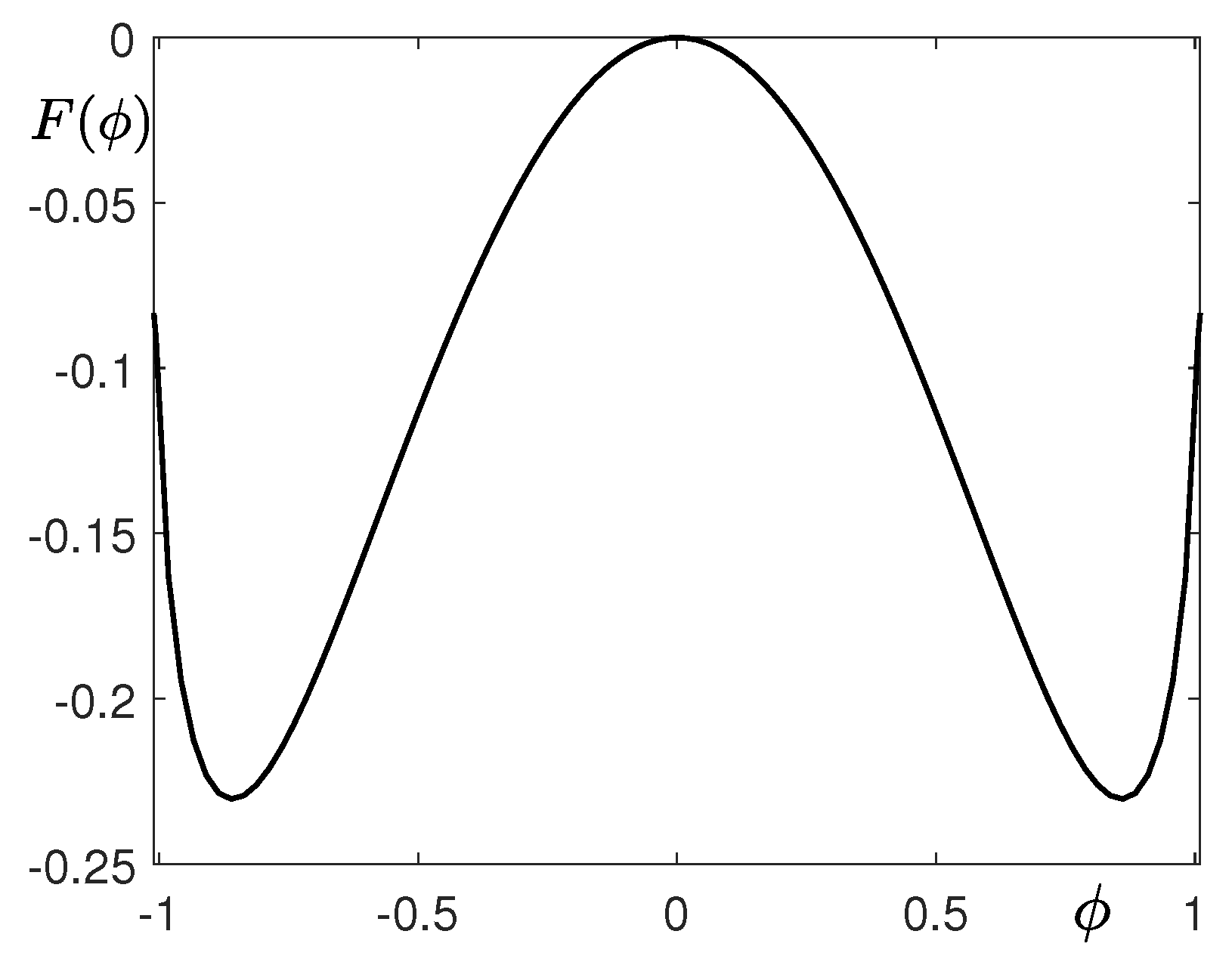
is the free energy potential, and
is a small constant related to the interfacial energy. Note that
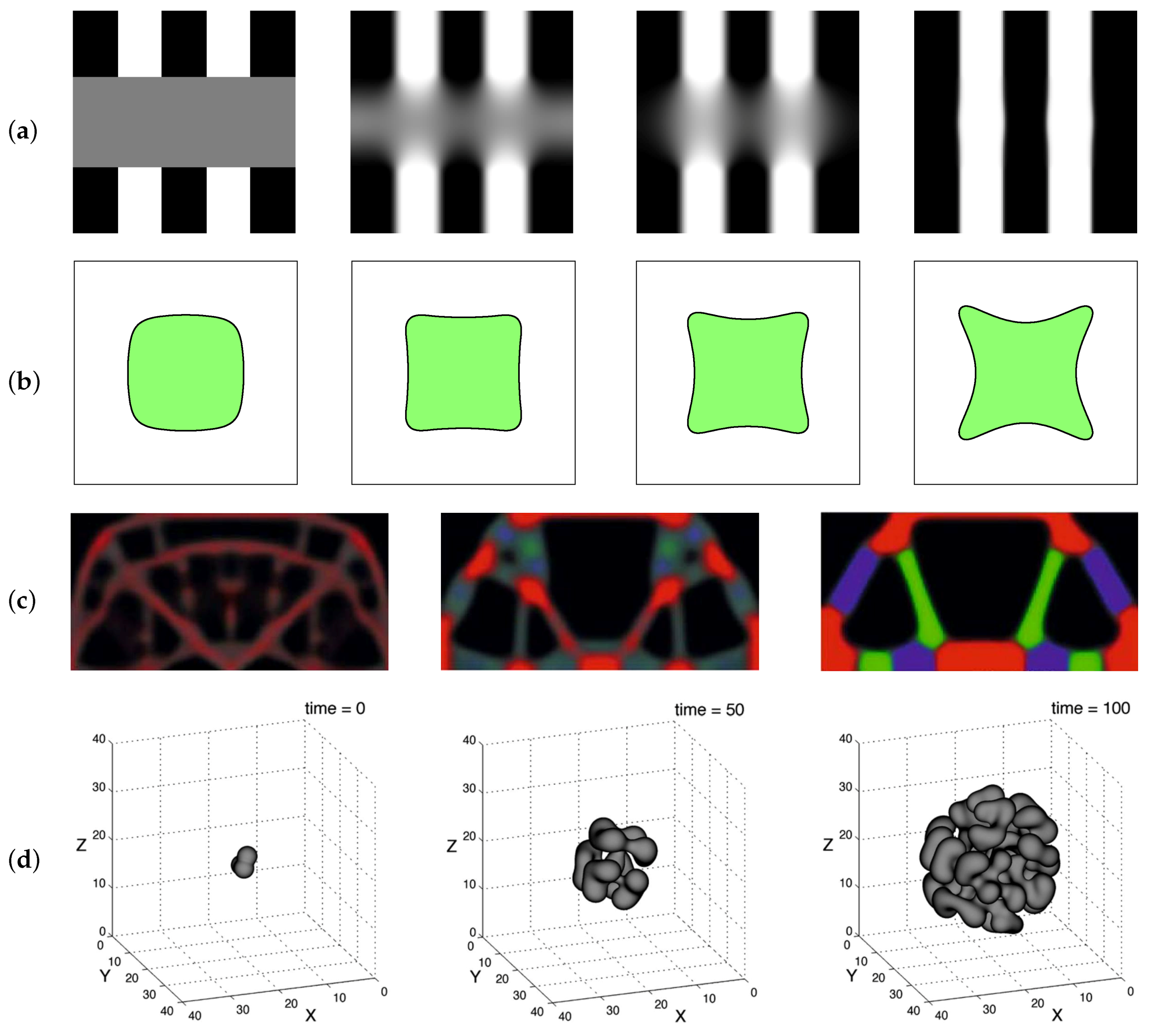
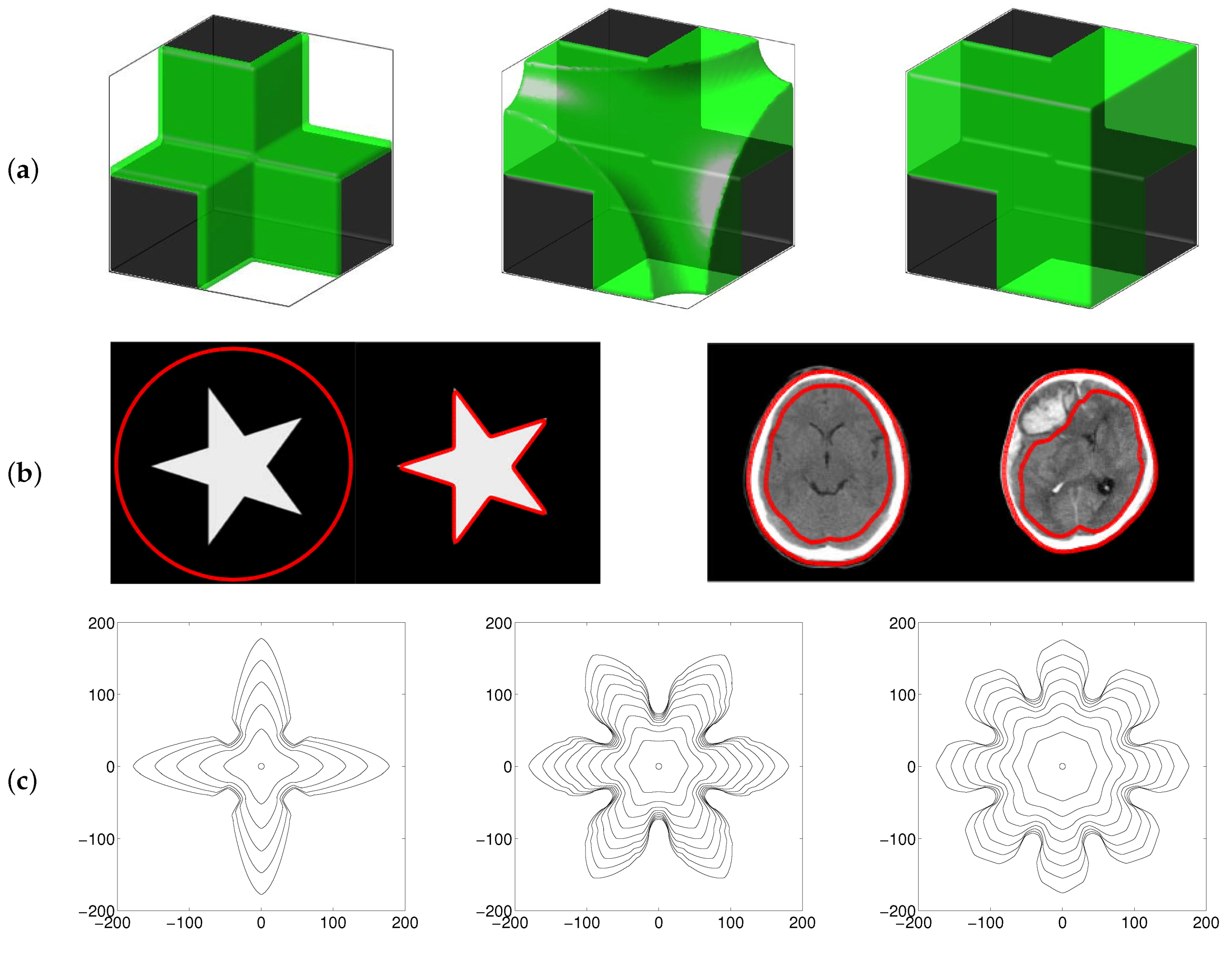
. The AC equation has a wide range of applications such as mean curvature flows, two-phase incompressible fluids, complex dynamics of dendritic growth, image inpainting, and image segmentation, see
Figure 4 for some of these examples [
5,
6,
7].
Lee and Lee [
8] presented unconditionally energy stable first- and second-order semi-analytical Fourier-spectral methods for the AC equation to reduce the errors caused by large time step. Those methods were originated by decomposition of original equation into two parts, linear and nonlinear, that have closed-form solutions; hence operator splitting steps ensure high-order nonlinear solvers.
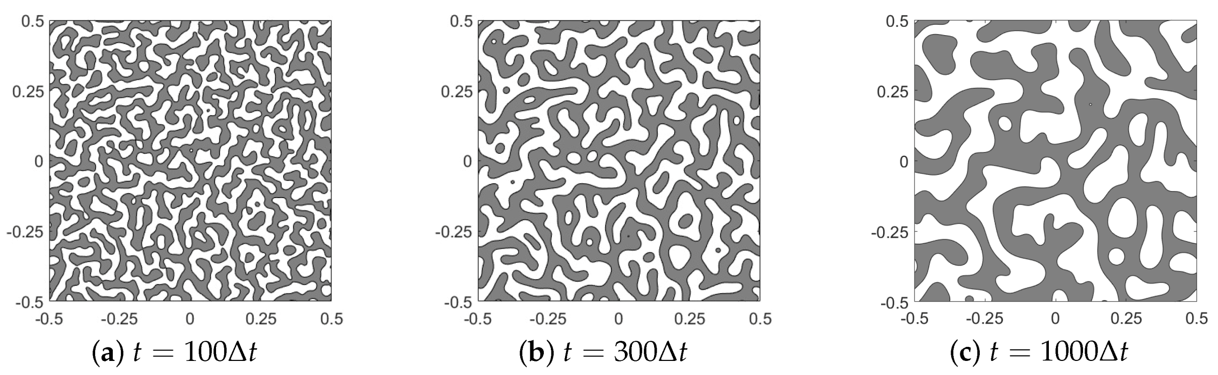
The next is a similar type to the previous one, the Cahn–Hilliard (CH) equation, which models the process of spinodal decomposition in conserved binary alloys [
9]:
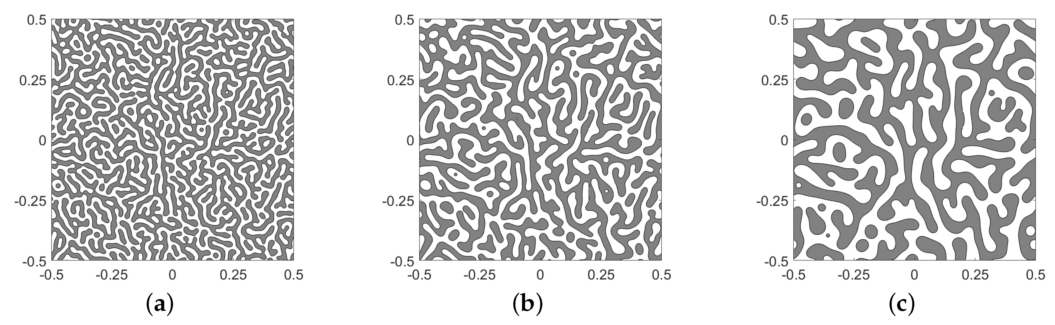
The CH equation is widely used in applications such as phase separation, topology optimization, multiphase incompressible fluid flows, image inpainting, surface reconstruction, diblock copolymer, tumor growth simulation, and microstructures with elastic inhomogeneity, see
Figure 5 for some of these examples [
10].
Recently in [
11], the discretization via nonlinear stabilized splitting scheme to the CH equation was reviewed and was solved by using a nonlinear multigrid method. Further in [
12], Lee researched energy stability of the second-order strong-stability-preserving implicit-explicit Runge–Kutta methods for the CH equation. Christlieb et al. [
13] presented the unconditionally gradient nonlinearly stabilized method for the CH equation, which is originally proposed by Eyre [
14], within Fourier method and proposed an iterative scheme which is convergent for large time steps. There are a bunch of research related in AC and CH equations so far, some selected literatures are listed as follows. Montanelli and Bootland [
15] proposed several exponential integration formula and compared their performance within stiff partial differential equations including AC and CH models. Such models are rewritten to sum of linear operator part with high-order terms and nonlinear operator part, and then Fourier-spectral method is applied in order to employ exponential integrator to this semilinear ordinary differential equations. Zhang and Liu [
16] used several AC or CH type equations to represent the spatial patterns in ecological and biological system. Shen and Yang [
17] presented numerical approximations of the AC and CH equations for semi-implicit or implicit schemes which are unconditionally energy stable, with stability analysis and error estimates based on spectral-Galerkin method. The results confirmed that spectral methods are suitable for diffusive interface models. Regarding on this respect especially, we introduce a nonlocal CH equation, which is appropriate to apply the Fourier-spectral method, that can model microphase separation in diblock copolymers, which consist of two different types of monomers [
18] and an explicit form is listed as follows:
where
is inversely proportional to the square of the total chain length of the copolymer and
is the average concentration over the domain
. Block copolymer is a linear-chain molecule consists of at least two subchains connected to each other to make a polymer chain. A diblock copolymer exists if the subchain consists of two distinct monomer blocks. Related mathematical models have been developed in order to investigate the behaviors of phase separation of block copolymers and to find an available technique to manufacture nano-structured materials [
19,
20,
21,
22]. There is a direct applications of Equation (
4) in [
23] recently, where the authors employ the spectral method and see the references therein to check more details.
The Swift–Hohenberg (SH) equation was originally derived to model patterns from the influence of thermal fluctuations in hydrodynamics [
24]:
where
is a density field and
is a temperature related positive constant. There are several applications to employ this model such as cellular materials, metallurgy, laser dynamics, electrohydrodynamics, crystallography, etc. See [
25,
26,
27,
28] and the references therein for more details. In addition, we introduce a classical phase field crystal (PFC) equation which takes account for atomic-crystallization growth [
29]:
This model has a variety of applications such as crystallization in liquid-liquid interface with undercooled material, isotropic phase separation, etc. On the atomistic/molecular scale freezing, a theoretical approach to undercooled liquids crystallization has been studied in [
30,
31], and the efficient numerical methods based on the operator splitting method or spectral method are developed for the phase-field crystal model [
32,
33]. The operator splitting method with Fourier-spectral method can relax the time step restriction or shorten the computation time depending on which a solver is applied for each stage.
A molecular beam epitaxy (MBE) growth model describes a process in which a thin single crystal layer is deposited on a single crystal substrate using molecular beams [
34,
35]:
The MBE model is a substantially used approach for thin-film deposition of a surface or interface quality determined to single-monolayer precision. This procedure is widely applied in semiconductor heterostructures and persistently studied topic in material science. Consequently, considerable mathematical models have been evolved to study the epitaxy dynamics, covering from continuum models to molecular dynamical simulations. The readers are referred to the following references for more details [
36,
37,
38,
39,
40,
41,
42,
43].
The main purpose of this paper is to present brief reviews, to describe numerical solution algorithms, and to provide the MATLAB code implementations of the unconditionally gradient stable Fourier-spectral method for the several phase-field equations. In particular, we highlight the caution that needs to be taken when applying the MATLAB based fast Fourier transform to the Fourier-spectral method.
The outline of this paper is as follows. The numerical solutions in two- and three-dimensional cases of the above phase-field models are described in
Section 2 and
Section 4, respectively. In
Section 3 and
Section 5, we present the basic numerical simulations to the stated phase-field models in both two- and three-dimensional cases. We finalize the paper with the conclusion in
Section 6. In the
Appendix A, we provide the MATLAB codes for the numerical implementation of the presented equations.
2. Numerical Solutions in 2D
In this section, we present unconditionally stable Fourier-spectral methods for the phase-field models in two-dimensional space
. Let
,
be positive even integers and
,
be the length of each direction, respectively; hence define
and
as the spatial step size in each direction, respectively. We denote discretized points as
where
and
are integers. Let
be an approximation of
, where
and
is the temporal step size. For the given data
and
, the discrete Fourier transform is defined as
where
and
. The inverse discrete Fourier transform is
Note that we can obtain spectral derivatives as if we perform analytic differentiations in the Fourier space. We assume that
is sufficiently smooth and extended to continuous version of the numerical approximation
. The following shows step-by-step description of how the differentiation works in the Fourier transform with finite basis.
This process enables one can derive spectral derivatives in the Fourier space easily, not differentiate directly in the physical space. Therefore, we can represent the Laplacian to coefficients in the Fourier space as follows:
where the first line is the definition of the inverse Fourier transform and the second line is just applying Equation (
10) twice to
x- and
y-direction to
and its Fourier transform.
Now we present the numerical solutions of phase-field equations. First, we derive the numerical solution of the AC equation. We apply the linearly stabilized splitting scheme [
14] to Equation (
2).
where
. Thus, Equation (
12) can be transformed into the discrete Fourier space as follows:
Therefore, we obtain the following discrete Fourier transform
Then, the updated numerical solution
can be computed using Equation (
9):
Next, we obtain the numerical solution of the CH equation. We employ the linearly stabilized splitting scheme [
14] to Equation (
3).
Thus, Equation (
16) can be transformed into the discrete Fourier space as follows:
Therefore, we obtain the following discrete Fourier transform
Then, the updated numerical solution
can be computed using Equation (
9):
Now, we present a numerical solution to the SH equation. In a similar manner, we discretize Equation (
5) as follows:
where
. Then we transform Equation (
20) as
Therefore, we have the following result
and hence we have a numerical solution
as follows:
Similarly, a numerical solution for the PFC model (
6) is obtained by the same procedure
Then Equation (
24) is transformed as
Therefore, we have the following result
Subsequently, we have a numerical solution
as follows:
The remaining one is a numerical solution to the MBE growth model (
7). Discretize Equation (
7) with an expanded divergence term
and treat this in implicit way,
We define
. Then Equation (
28) is transformed as
where
is
Note that
and
represent the discrete Fourier transform and the discrete inverse Fourier transform, respectively. Therefore, we have the following result
and then we update a numerical solution
as follows:
4. Numerical Solutions in 3D
We extend the Fourier-spectral method on two-dimensional space to three-dimensional space,
for the stated phase-field models. Let
,
,
be positive even integers and
,
,
be the length of each direction, respectively. We denote discretized points by
for
,
,
, where
,
,
is the spatial step size in each direction, respectively. For
,
is denoted by
, where
is the temporal step. For the given data
,
,
, the discrete Fourier transform is defined as
where
,
,
. The inverse discrete Fourier transform is
Similar to the two-dimensional case, we assume that
is sufficiently smooth and extended to continuous version of the numerical approximation
. Therefore, we can obtain the following result.
Consequently, we can write Laplacian as coefficients in the Fourier space as follows:
where the first line is the definition of the inverse Fourier transform and the second line is just applying Equation (
67) twice to
x-,
y-, and
z-direction to
and its Fourier transform. Now, we present the numerical solutions of three-dimensional phase-field models. Since most of the calculations are redundant, we just briefly list as follows by extending the solvers in two-dimensional space to those of three-dimensional space. Note that the functions
f and
g which are defined in
Section 2 are simply extended to three-dimensional domain. The following is a numerical solution to the AC Equation (
2).
Then, the renewed numerical solution
can be computed using Equation (
66):
Next one is a numerical solution to the CH Equation (
3).
Then, the renewed numerical solution
can be calculated using Equation (
66):
The following is a numerical solution to the SH Equation (
5).
and hence we have a numerical solution
as follows:
Subsequently, we have a numerical solution to the classical PFC model (
6) as follows.
Therefore, we have a numerical solution
as follows:

 ,
, 


