Optimal Auxiliary Functions Method for a Pendulum Wrapping on Two Cylinders

Abstract
:1. Introduction
2. The Optimal Auxiliary Functions Method
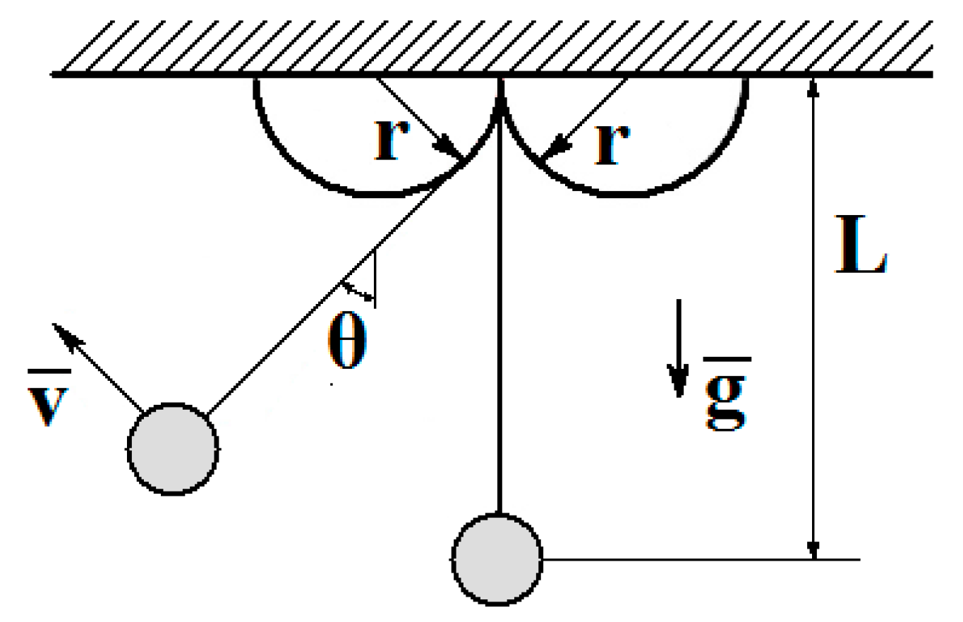
3. Equation of Motion
4. Application of OAFM to a Pendulum Wrapping on Two Cylinders
5. Results and Discussion
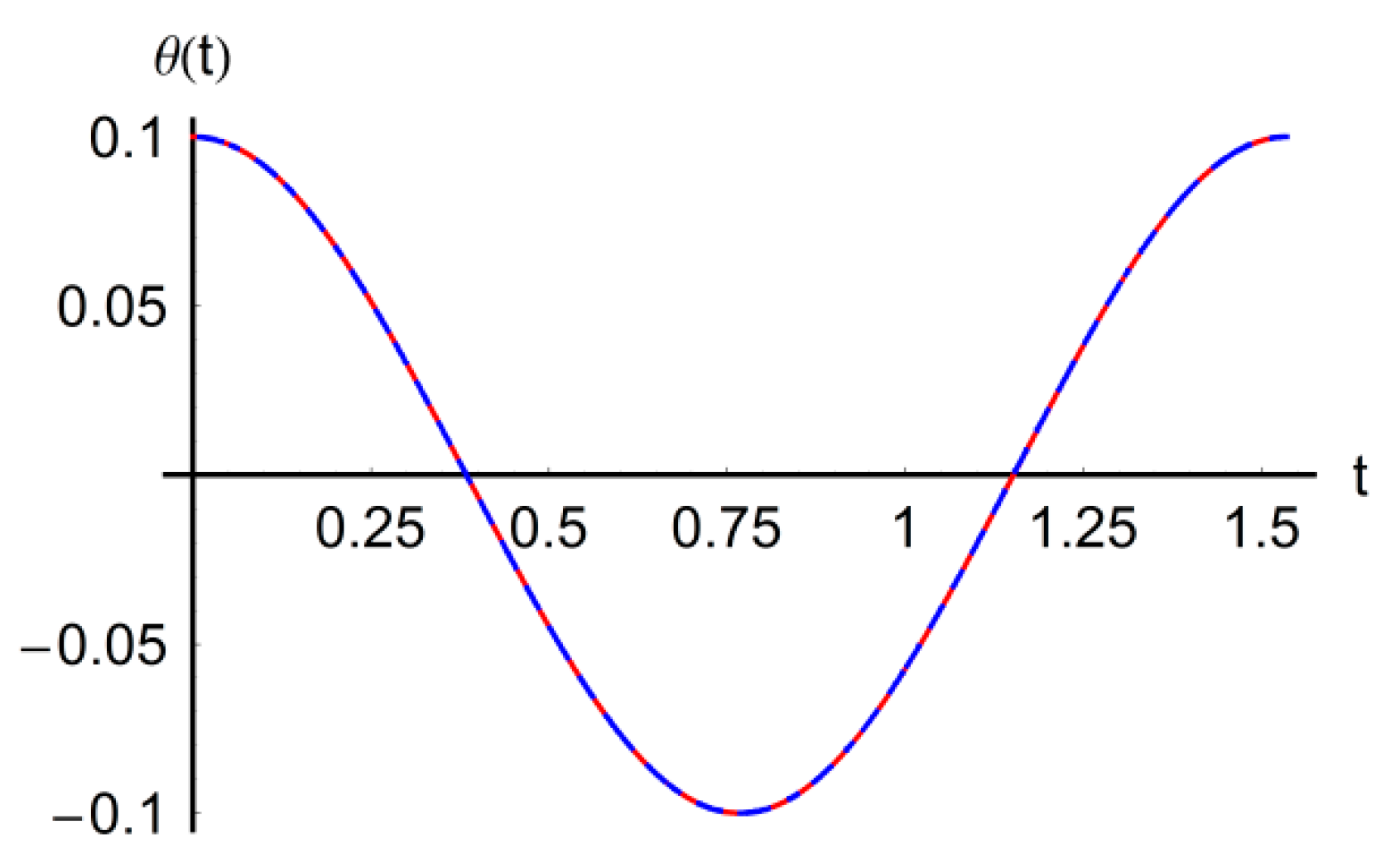
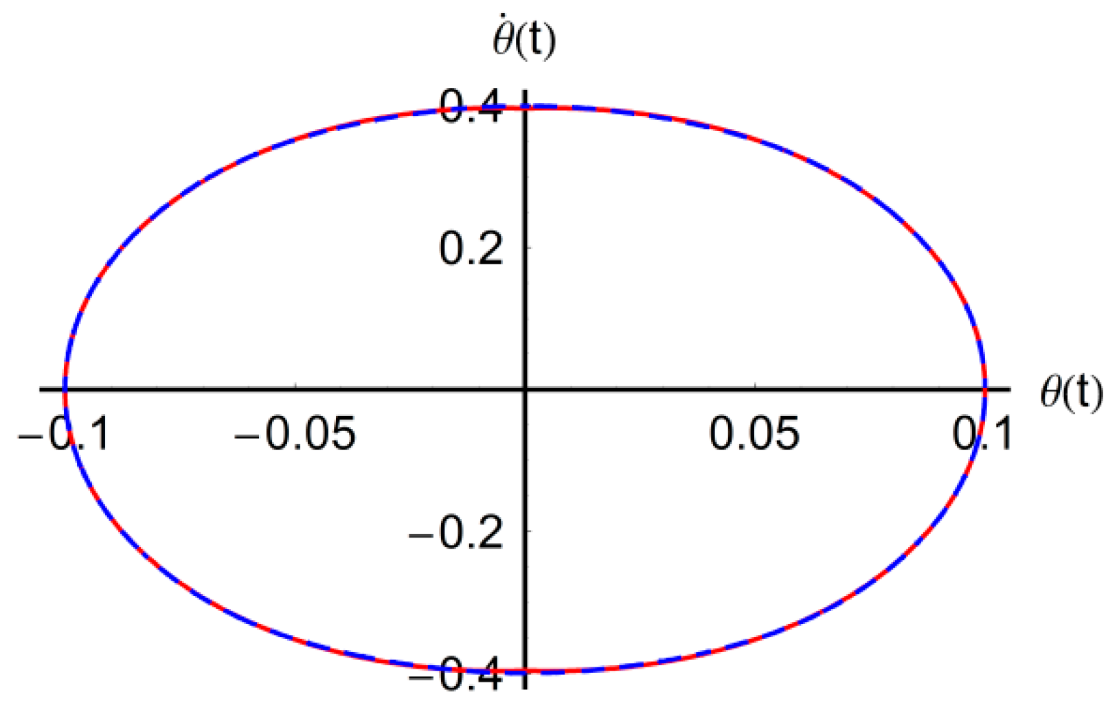
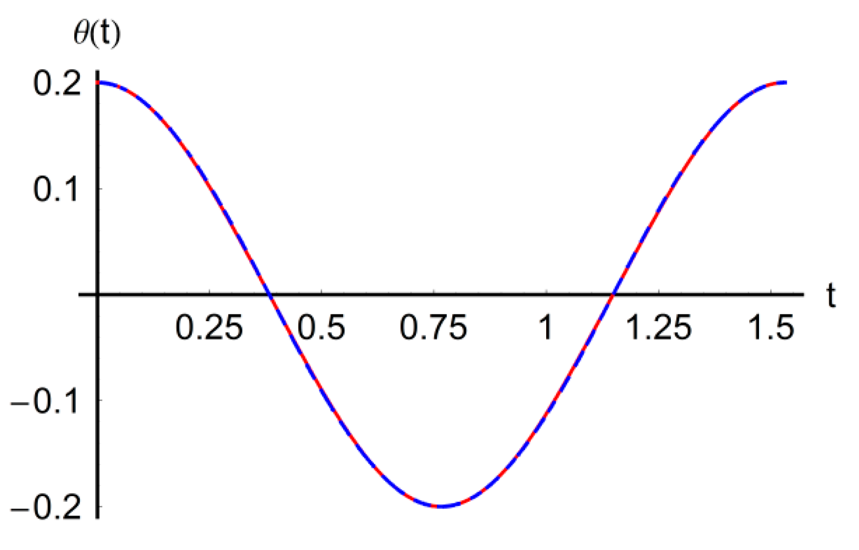
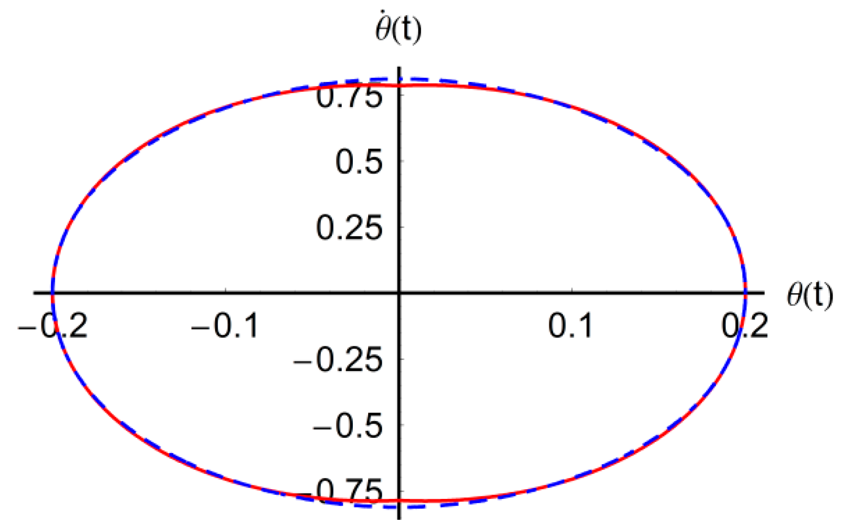
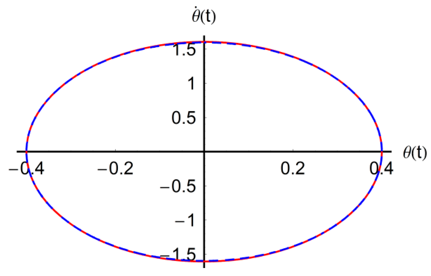
5.1. Case 1
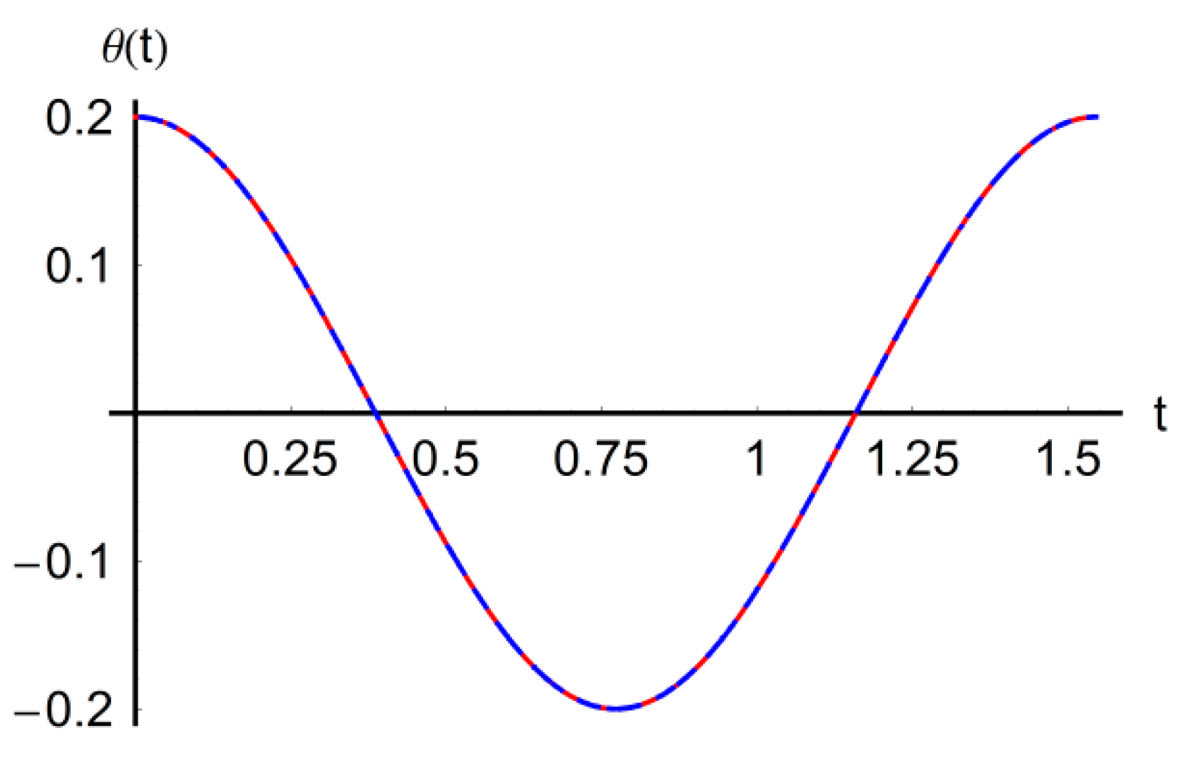
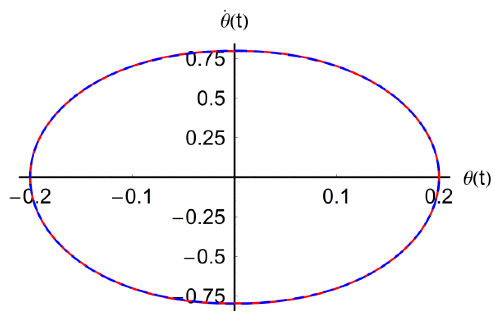
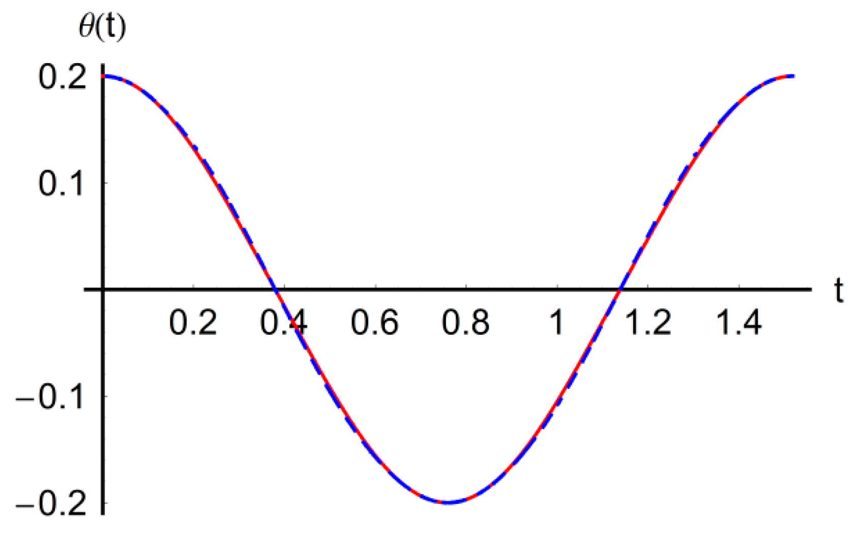
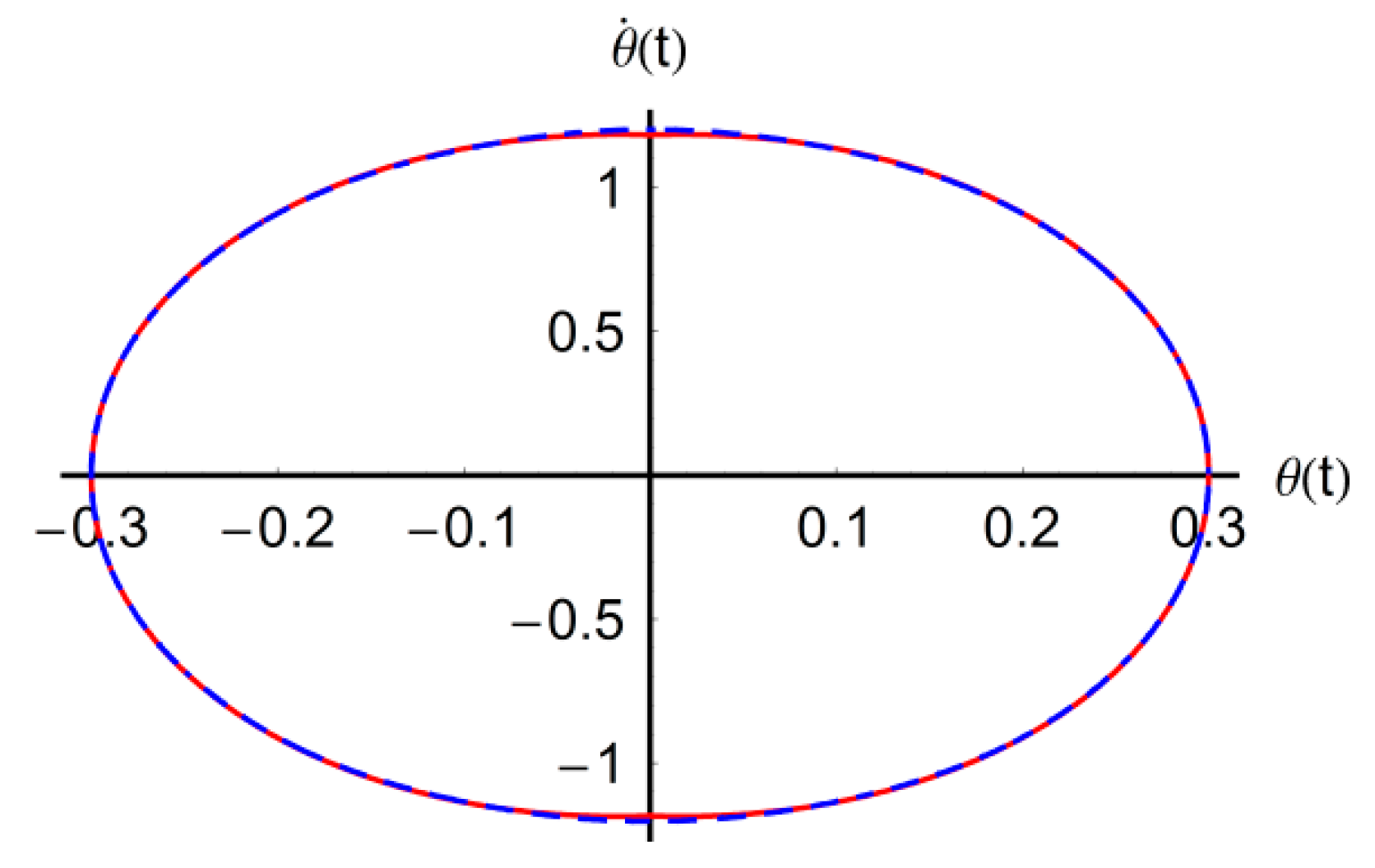
5.2. Case 2
5.3. Case 3
5.4. Case 4
5.5. Case 5
5.6. Case 6
5.7. Case 7
5.8. Case 8
5.9. Case 9
5.10. Case 10
6. Conclusions
Author Contributions
Funding
Conflicts of Interest
References
- Stillman, D. Galileo at Work: His Scientific Biography; Courier Corporation: North Chelmsford, MA, USA; Dover Corporation: Downers Grove, IL, USA, 2003. [Google Scholar]
- Matthews, R.M. Time for Science Education: How Teaching the History and Philosophy of Pendulum Motion Can Contribute to Science Literacy; Springer: New York, NY, USA, 2000. [Google Scholar]
- Aczel, A. Leon Foucault: His life, times and achievements. In The Pendulum: Scientific, Historical, Educational and Philosophical Perspectives; Matthews, M.R., Gauld, C.F., Stinner, A., Eds.; Springer: Berlin/Heidelberg, Germany, 2005; pp. 171–184. [Google Scholar]
- Marrison, W. The evolution of the quartz crystal clock. Bell Syst. Tech. J. 1948, 27, 510–588. [Google Scholar] [CrossRef]
- Audoin, C.; Guinot, B.; Lyle, S. The Measurement of Time, Frequency and the Atomic Clock; Cambridge University Press: Cambridge, UK, 2001. [Google Scholar]
- Willis, M. Time and Timekeepers; MacMillan: New York, NY, USA, 1945. [Google Scholar]
- Airy, G.B. On the disturbances of pendulum and balances and on the theory of escapements. Trans. Camb. Philos. Soc. 1830, III, 105–128. [Google Scholar]
- Lenzen, V.F.; Multauf, R.P. Development of Gravity Pendulums in the 19-th Century; United States National Museum Bulletin: Washington, DC, USA, 1964; Volume 240. [Google Scholar]
- Hamouda, M.N.H.; Pierce, G.A. Helicopter vibration suppression using simple pendulum absorbers on the rotor blade. J. Am. Helicopter Soc. 1984, 23, 19–29. [Google Scholar] [CrossRef] [Green Version]
- Nelson, R.A.; Olsson, M.G. The pendulum-Rich physics from a simple system. Am. J. Phys. 1986, 54, 112–121. [Google Scholar] [CrossRef]
- Ge, Z.M.; Ku, F.N. Subharmonic Melnikov functions for strongly odd nonlinear oscillators with large perturbations. J. Sound Vib. 2000, 236, 554–560. [Google Scholar] [CrossRef] [Green Version]
- Nester, T.M.; Schnitz, P.M.; Haddow, A.G.; Shaw, S.W. Experimental Observations of Centrifugal Pendulum Vibration Absorber. In Proceedings of the 10th International Symposium on Transport Phenomena and Dynamics of Rotating Machinery (ISROMAC-10), Honolulu, HI, USA, 7 March 2004. [Google Scholar]
- Bendersky, S.; Sandler, B. Investigation of a spatial double pendulum: An engineering approach. Discret. Dyn. Nat. Soc. 2006, 2006, 25193. [Google Scholar] [CrossRef] [Green Version]
- Horton, B.; Sieber, J.; Thompson, J.M.T.; Wiercigroch, M. Dynamics of the nearly parametric pendulum. Int. J. Nonlinear Mech. 2011, 46, 436–442. [Google Scholar] [CrossRef] [Green Version]
- Warminski, J.; Kecik, K. Autoparametric vibrations of a nonlinear system with pendulum. Math. Probl. Eng. 2006, 2006, 80705. [Google Scholar] [CrossRef]
- Kecik, K.; Warminski, J. Dynamics of anautoparametric pendulum-like system with a nonlinear semiactive suspension. Math. Probl. Eng. 2011, 2011, 451047. [Google Scholar] [CrossRef] [Green Version]
- Rafat, M.Z.; Wheatland, M.S.; Bedding, T.R. Dynamics of a double pendulum with distributed mass. Am. J. Phys. 2009, 77, 216–222. [Google Scholar] [CrossRef] [Green Version]
- Turkilazoglu, M. Accurate analytic approximation to the nonlinear pendulum problem. Phys. Scr. 2011, 84, 015005. [Google Scholar] [CrossRef]
- Awrejcewicz, J. Classical mechanics: Dynamics. Advances in Mechanics and Mathematics; Springer: Berlin/Heidelberg, Germany, 2012. [Google Scholar]
- Ludwicki, M.; Awrejcewicz, J.; Kudra, G. Spatial double physical pendulum with axial excitation—Computer simulation and experimatal set-up. Int. J. Dyn. Control. 2015, 3, 1–8. [Google Scholar] [CrossRef] [Green Version]
- Starosta, R.; Sypniewska-Kaminska, G.; Awrejcewicz, J. Parametric and external resonances in kinematically and externally excited nonlinear spring pendulum. Int. J. Bifurc. Chaos 2011, 21, 3013–3021. [Google Scholar] [CrossRef]
- Bayat, M.; Pakar, I.; Bayat, M. Application of He’s energy balance method for pendulum attached to rolling wheels that are restrained by a spring. Int. J. Phys. Sci. 2012, 7, 913–921. [Google Scholar]
- Mazaheri, H.; Hosseinzadeh, A.; Ahmadian, M.T. Nonlinear oscillation analysis of a pendulum wrapping on a cylinder. Sci. Iran. B 2012, 119, 335–340. [Google Scholar] [CrossRef] [Green Version]
- Boubaker, O. The inverted pendulum benchmark in nonlinear control theory: A survey. Int. J. Adv. Robot. Syst. 2013, 10, 1–5. [Google Scholar] [CrossRef] [Green Version]
- Alevras, P.; Yurchenko, D.; Naess, A. Stochastic synchronization of rotating parametric pendulums. Meccanica 2014, 49, 1945–1951. [Google Scholar] [CrossRef]
- Jallouli, A.; Kacem, N.; Bouhaddi, N. Stabilization of solitons in coupled nonlinear pendulums with simultaneous external and parametric excitation. Commun. Nonlinear Sci. Numer.Simul. 2017, 42, 1–11. [Google Scholar] [CrossRef] [Green Version]
- Herisanu, N.; Marinca, V. An effcient analytical approach to investigate the dynamics of a misaligned multirotor system. Mathematics 2020, 8, 1083. [Google Scholar] [CrossRef]
- Herisanu, N.; Marinca, V.; Madescu, G.; Dragan, F. Dynamic response of a permanent magnet synchronous generator to a wind gust. Energies 2019, 12, 915. [Google Scholar] [CrossRef] [Green Version]
- Marinca, V.; Herisanu, N. An optimal iteration method with application to the Thomas-Fermi equation. Cent. Eur. J. Phys. 2011, 9, 891–895. [Google Scholar] [CrossRef]
- Marinca, V.; Herisanu, N. Explicit and exact solutions to cubic Duffing and double-well Duffing equations. Math. Comput. Model. 2011, 53, 604–609. [Google Scholar] [CrossRef]
- Fu, C.; Xu, Y.; Yang, Y.; Lu, K.; Gu, F.; Ball, A. Dynamics analysis of a hollow-shaft rotor system with an open crack under model uncertainties. Commun. Nonlinear Sci. Numer. Simul. 2020, 83, 105102. [Google Scholar] [CrossRef]
- Fu, C.; Zhen, D.; Yang, Y.; Gu, F.; Ball, A. Effects of bounded uncertainties on the dynamic characteristics of an overhung rotor system with rubbing fault. Energies 2019, 12, 4365. [Google Scholar] [CrossRef] [Green Version]
- Li, H.; Chen, Y.; Hou, L.; Zhang, Z. Periodic response analysis of a misaligned rotor system by harmonic balance method with alternating frequency/time domain technique. Sci. China Technol. Sci. 2016, 59, 1717–1729. [Google Scholar] [CrossRef]
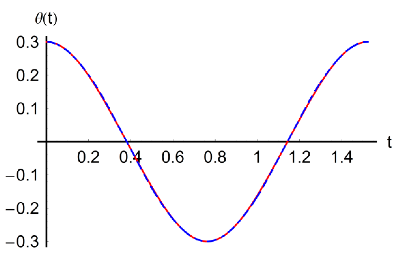
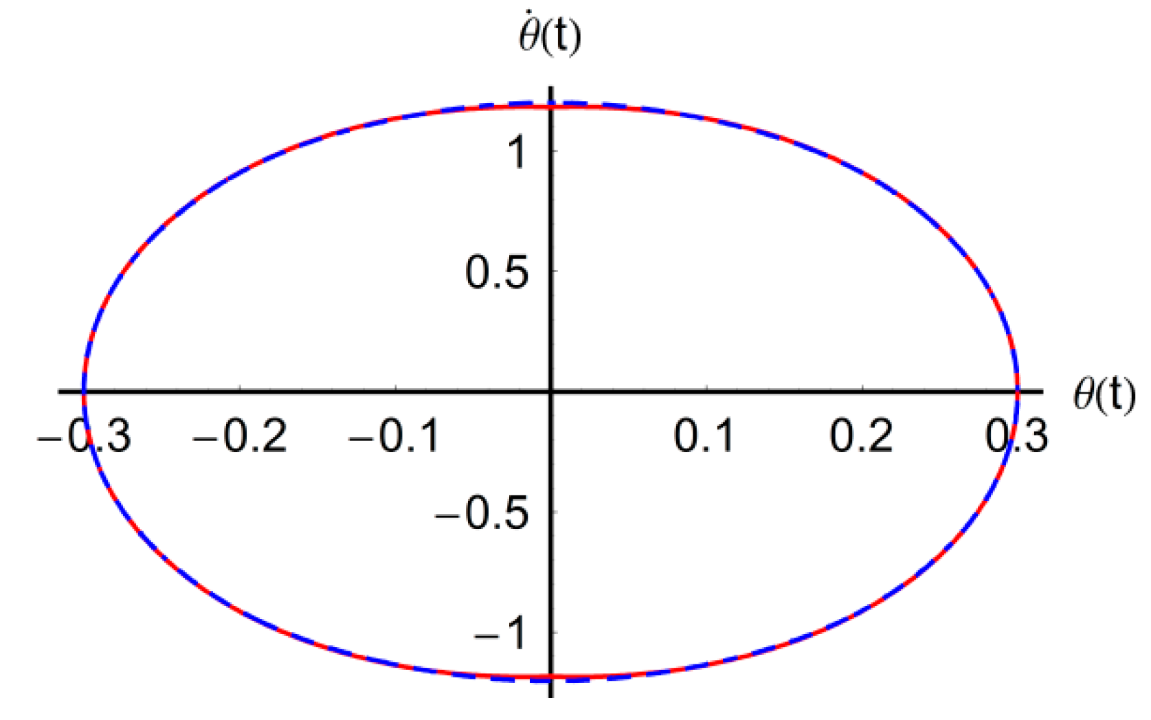
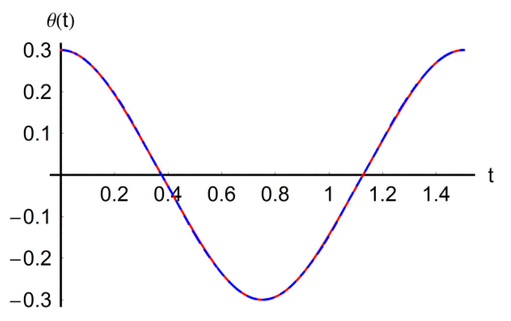
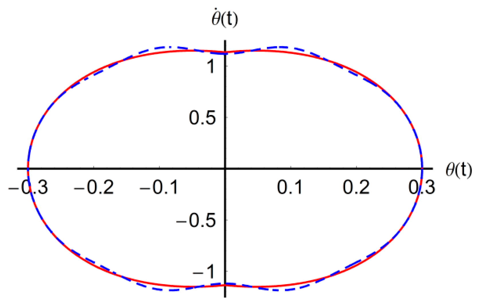
 numerical
  approximate solution.
numerical approximate solution.
approximate solution.
numerical approximate solution.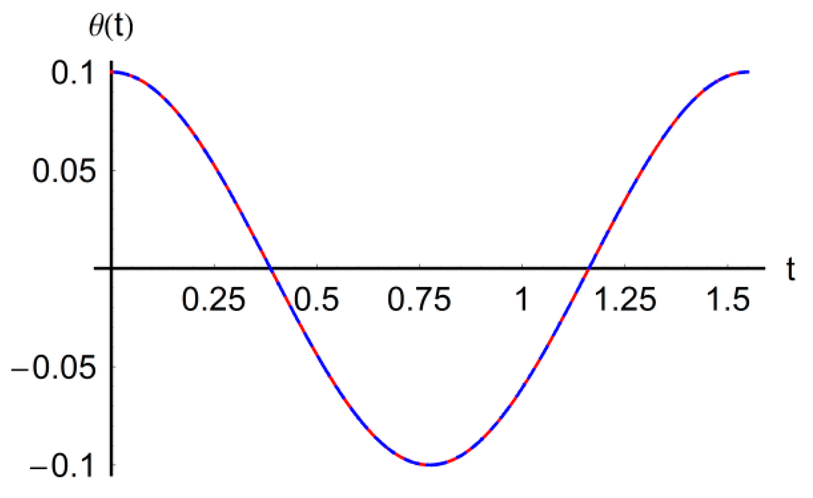 numerical approximate solution (39).
 numerical approximate solution.
numerical approximate solution.
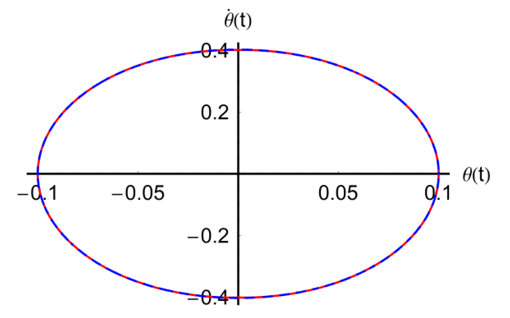
numerical approximate solution.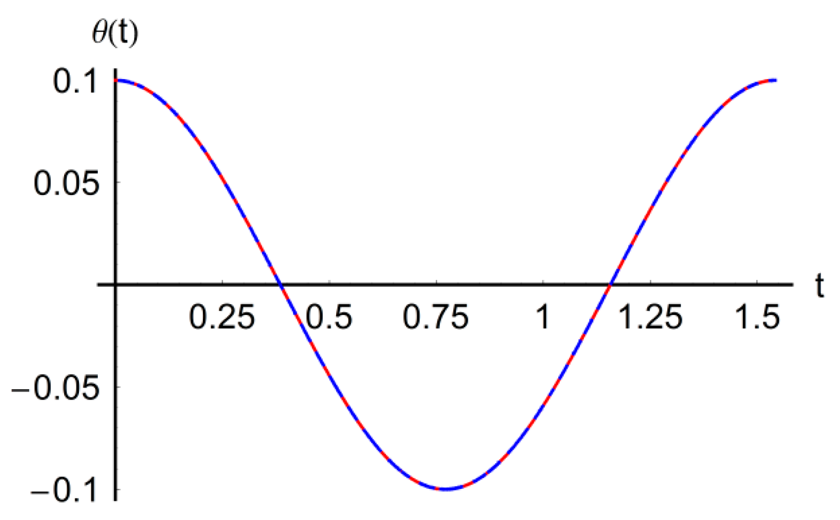 numerical approximate solution (40).
 numerical approximate solution.
numerical approximate solution.
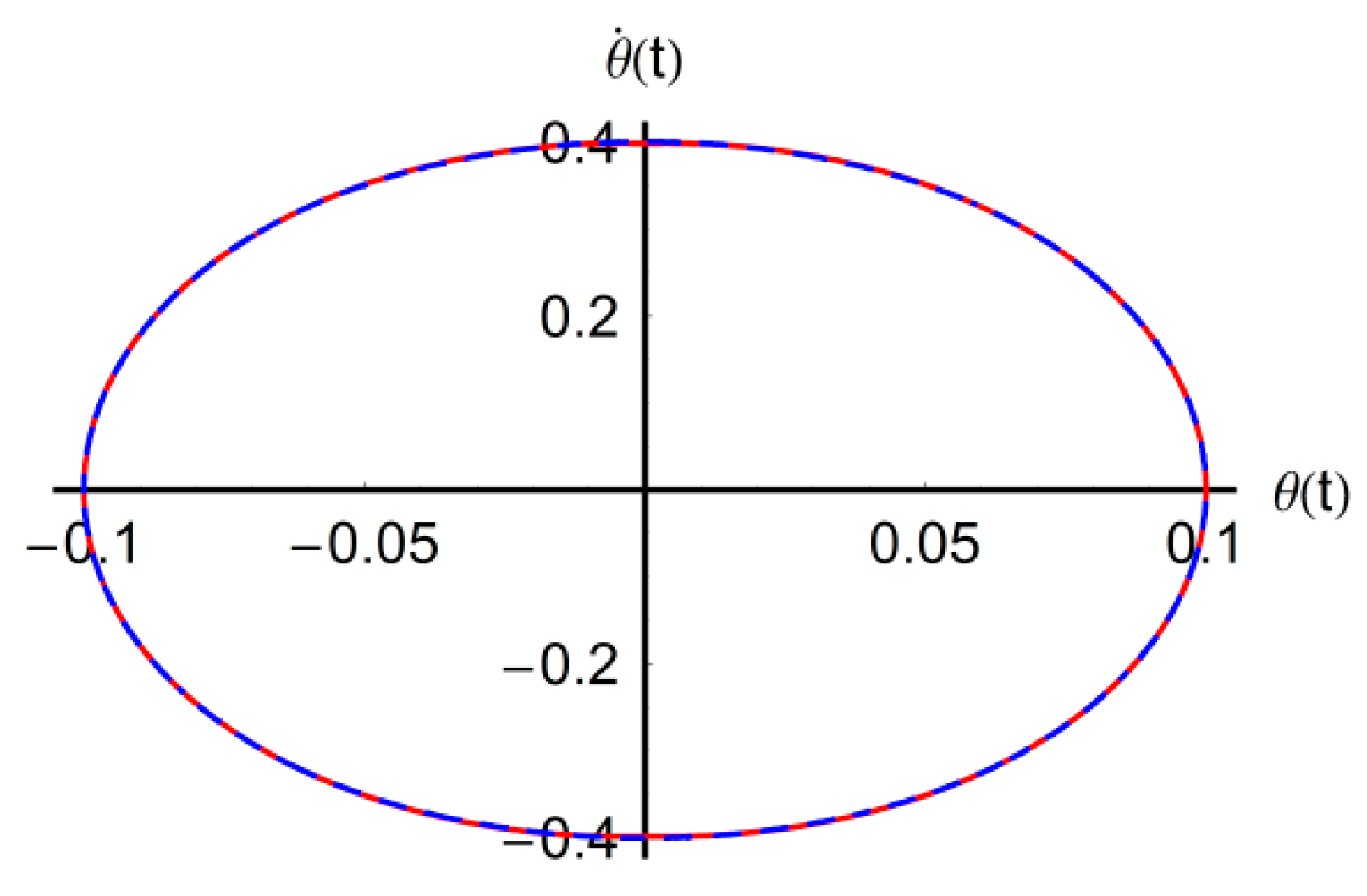
numerical approximate solution. numerical approximate solution (41).
 numerical approximate solution.
numerical approximate solution.
numerical approximate solution. numerical approximate solution (42).
 numerical approximate solution.
numerical approximate solution.
numerical approximate solution. numerical approximate solution (43).
 numerical approximate solution.
numerical approximate solution.
numerical approximate solution. numerical approximate solution (44).
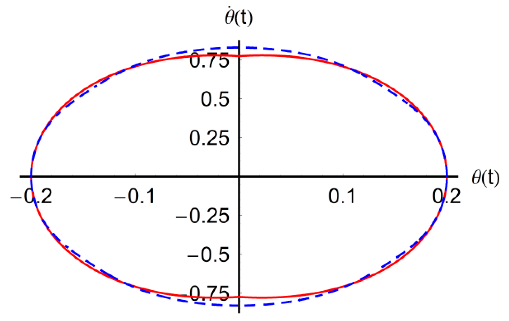 numerical approximate solution.
numerical approximate solution.
numerical approximate solution.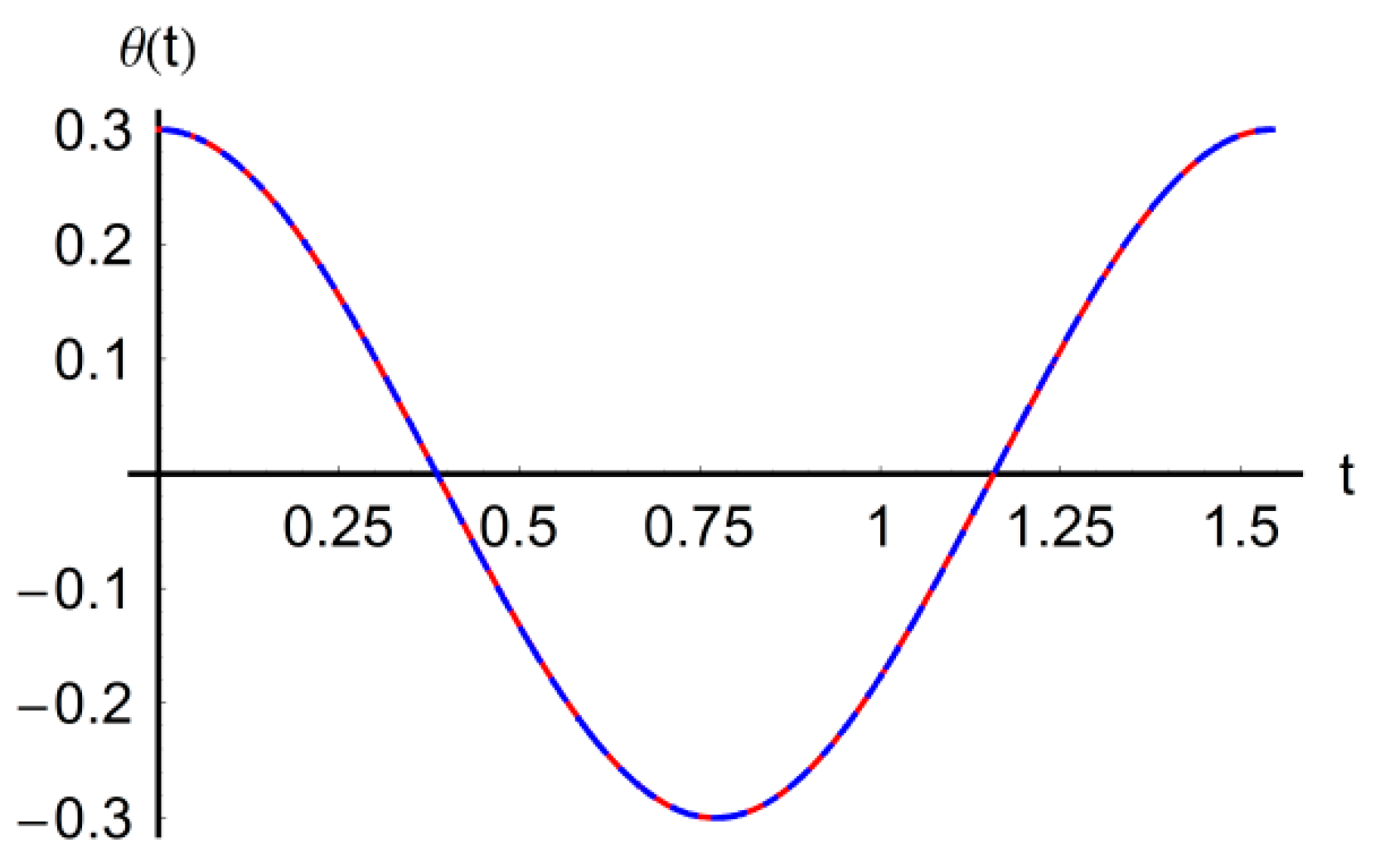 numerical approximate solution (45).
 numerical approximate solution.
numerical approximate solution.
numerical approximate solution. numerical approximate solution (46).
 numerical approximate solution.
numerical approximate solution.
numerical approximate solution. numerical approximate solution (47).
 numerical approximate solution.
numerical approximate solution.
numerical approximate solution.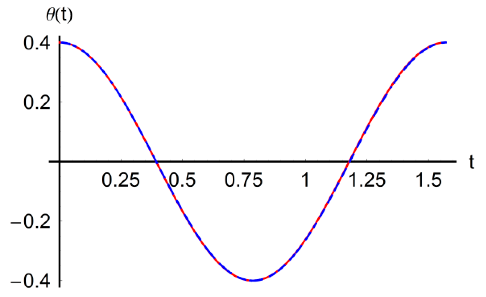 numerical approximate solution (50).

| Case No. | Ωnum | Ωapp |
|---|---|---|
| 5.1 | 4.056165704763733 | 4.056213309077129 |
| 5.2 | 4.0735936668241015 | 4.0735339712576275 |
| 5.3 | 4.091213341156173 | 4.091781570513826 |
| 5.4 | 4.065980106247986 | 4.0659463540564085 |
| 5.5 | 4.10137202740024 | 4.1008614227769575 |
| 5.6 | 4.137539732217073 | 4.137450803506345 |
| 5.7 | 4.070864763571452 | 4.071192550653585 |
| 5.8 | 4.124733651749398 | 4.125254940744536 |
| 5.9 | 4.180380645932648 | 4.180777463105995 |
© 2020 by the authors. Licensee MDPI, Basel, Switzerland. This article is an open access article distributed under the terms and conditions of the Creative Commons Attribution (CC BY) license (http://creativecommons.org/licenses/by/4.0/).
Share and Cite
Marinca, V.; Herisanu, N. Optimal Auxiliary Functions Method for a Pendulum Wrapping on Two Cylinders. Mathematics 2020, 8, 1364. https://doi.org/10.3390/math8081364
Marinca V, Herisanu N. Optimal Auxiliary Functions Method for a Pendulum Wrapping on Two Cylinders. Mathematics. 2020; 8(8):1364. https://doi.org/10.3390/math8081364
Chicago/Turabian StyleMarinca, Vasile, and Nicolae Herisanu. 2020. "Optimal Auxiliary Functions Method for a Pendulum Wrapping on Two Cylinders" Mathematics 8, no. 8: 1364. https://doi.org/10.3390/math8081364
APA StyleMarinca, V., & Herisanu, N. (2020). Optimal Auxiliary Functions Method for a Pendulum Wrapping on Two Cylinders. Mathematics, 8(8), 1364. https://doi.org/10.3390/math8081364