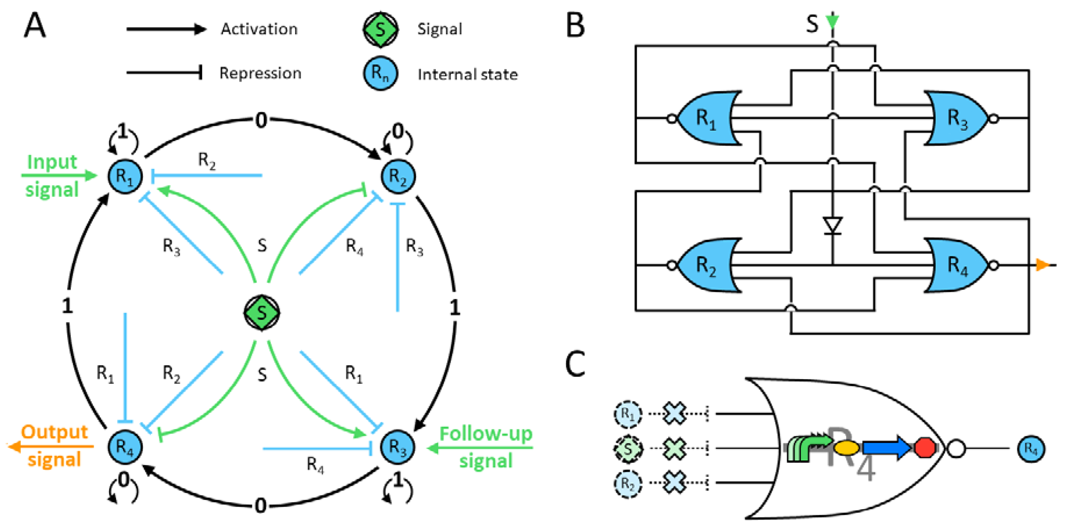
3.1. Deterministic Model
The designed genetic circuit is depicted in
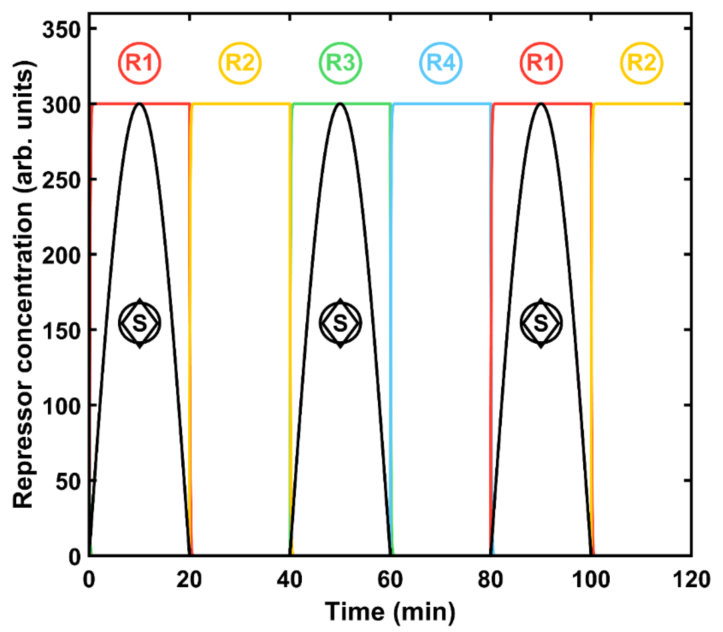
Figure 1, and the corresponding protein evolution is displayed in
Figure 2. The four-state automaton starts with the genetic construct producing the repressor protein R
1. Only when there is a signal can it be activated, i.e., remains in state 1. Since the other repressors are absent, the machine stays in this state while the signal is present (
Figure 2). Once the latter disappears, R
1 proteins cannot be built up any more. Moreover, these factors have no inhibitory effect on the next state construct by design. The production of R
2 starts once the signal inhibition has faded and the next two repressors are still absent in the system. Remarkably, any previous-state repressor does not affect the promoter of the next-state construct. Hence, the system shifts to R
2 and stays in this state while there is no signal. In addition, the R
1 proteins are gradually degraded and their concentration vanishes. Next, a second input signal appears; it represses the promoter of R
2 and activates the one of R
3 (
Figure 2). Again, since there are no transcription factors of the next two states, the machine will remain in this state while the signal is on. Finally, the same principles apply for the last state, that is R
4, but this construct also produces an output signal that can be externally measured. In summary, the automaton shows a robust and expected output for each state, while the others remain close to zero.
Regarding the effect of the initial conditions, if only a tiny amount of R1 is present, the system can shift state in a consistent manner. If instead of this, the system starts from zero-protein conditions, R1 and R3 appear under signal presence as expected, and their maximal concentrations are around six times lower (data not shown). Increasing the initial concentration of R1 does not affect the automaton behavior as long as there are no other proteins present.
The steady-state concentration is equal to the ratio of protein production to degradation given by the respective coefficients , that is, 300 concentration units for our case study. Therefore, the repressor effects are negligible in the coherent design: there is no effective repression when one state dominates over the rest.
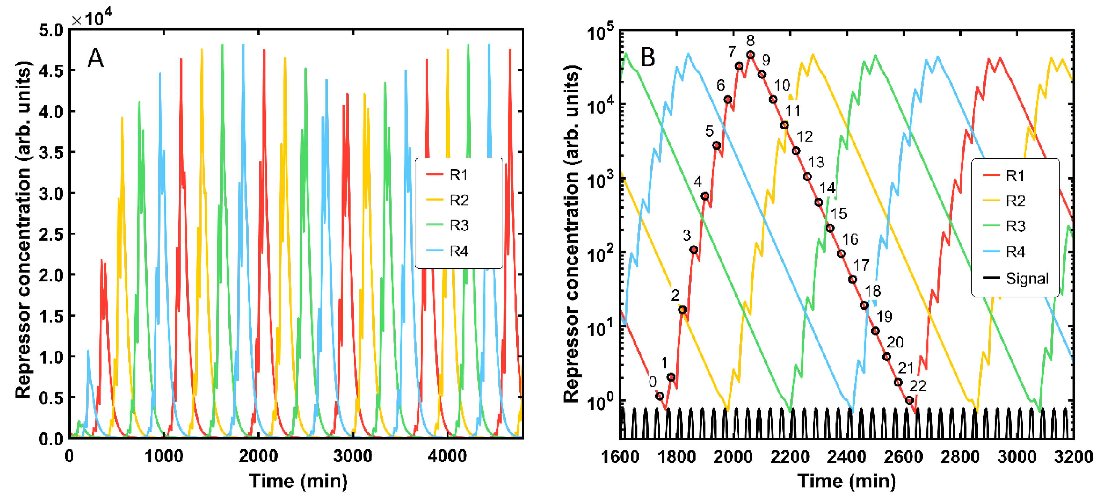
The genetic FSM is a complex system whose functionality is rather sensitive to changes in the magnitude of particular parameters. To illustrate this fact, we evaluated the performance of the automaton with the same parameter set as in the base case of a robust-functionality machine, but assuming a reduced protein degradation rate
, which is now considered to be 50 times lower (
). Interestingly, the system displays an altered response (
Figure 3). First, time scales and protein concentrations are now an order of magnitude higher. Counterintuitively, the maximal machine output takes much longer to be delivered, though the repressor amounts are considerably higher (
Figure 3A). Indeed, the automaton does not display fully robust behavior since many more input signals are required for reaching one machine cycle. The protein levels do not follow any sequential chain and display a sharper shape. In addition, abrupt concentration changes are visible at each signal shift. To further investigate the described effects, the protein concentrations were plotted in a semilogarithmic plot and focused on the time scale of a single machine cycle (
Figure 3B). Two different system responses can be distinguished: a local one affected by any new input signal (the abrupt slope changes) and an overall one, which is on a longer time scale. Hence, the FSM is still operating, as it was intended, but at another pace. In fact, 22 input signals are necessary to reach the same state again instead of two stimuli as in the standard design: eight for reaching the state peak, and another fourteen for the lowest value. In general, if the degradation rate is divided by k, then the whole cycle is k-times longer.
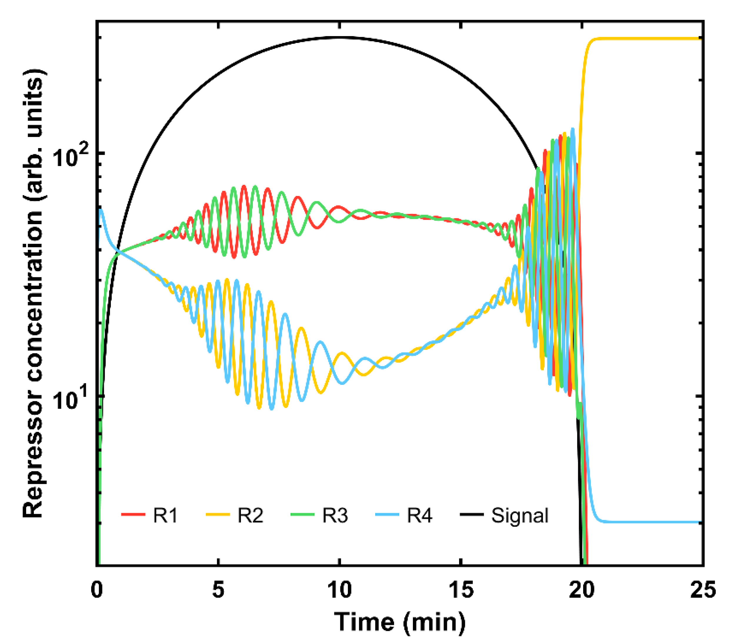
Another interesting experiment can be carried out when asymmetries are introduced in the system by considering a different effect of the input signal regarding its activation (R
1, R
3) and inhibition capacity (R
2, R
4). We hypothesize that the molecule representing the signal is capable of stronger activation of the promoter responsible for the production of the proteins R
1 and R
3, while efficiently repressing the others. The corresponding parameters are now assumed to be
,
. In
Figure 4, the system displays oscillatory behavior as the signal emerges.
Remarkably, the four states are coupled, sharing the same concentration magnitude within state blocks (red and green curves vs. yellow and blue ones). As long as the signal remains at a high level, both blocks remain approximately constant. However, once it starts to disappear, all states enter a strong feedback loop that is resolved once the signal is over and the second state rules over the rest. Once the system receives another signal, the same oscillatory phenomenon arises. Similarly, the signal amplitude has a clear impact on the device. When it is very low, below one unit, the evolution of the protein content starts to oscillate when the signal is present, but for even lower signal values, the R2 protein becomes predominant and its concentration is constant over time (data not shown).
3.2. Stochastic Model
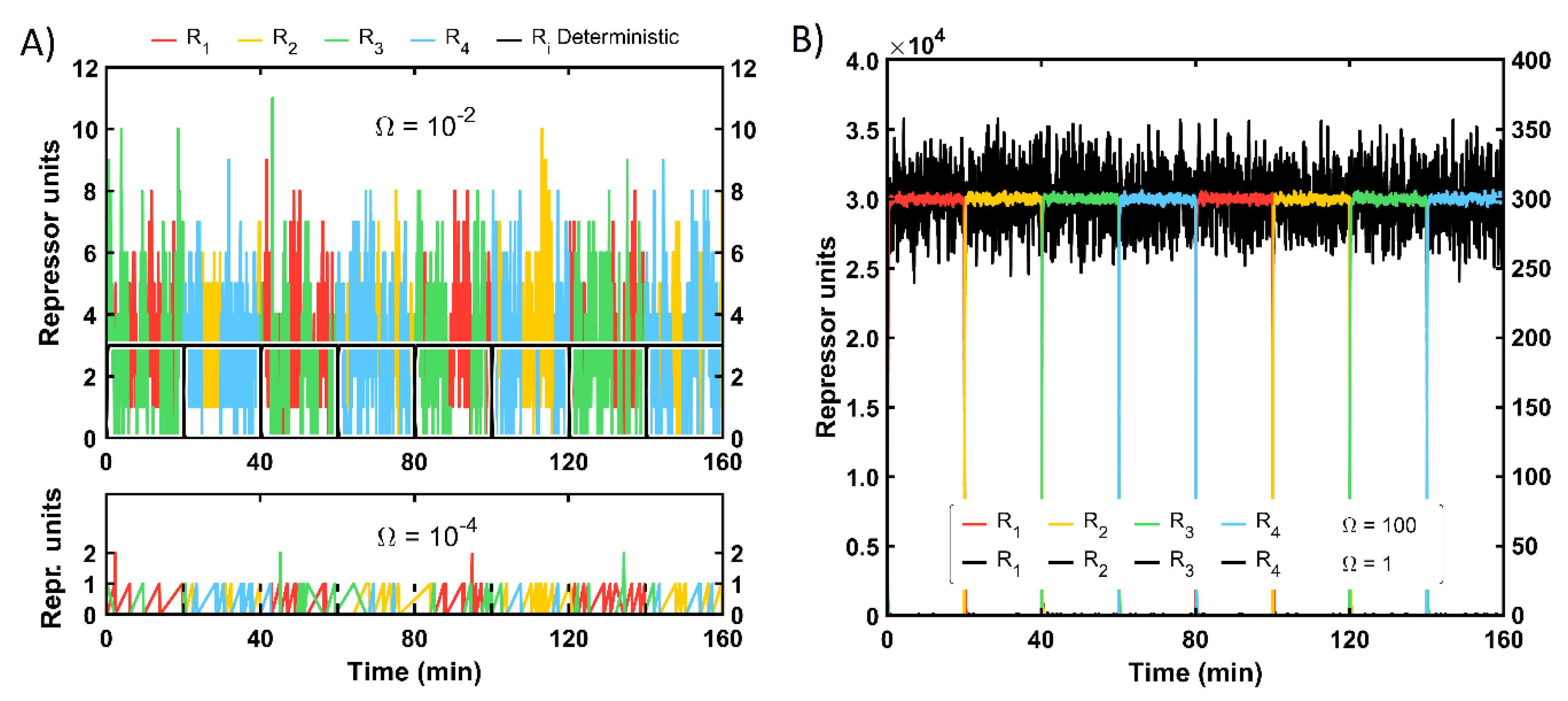
For the stochastic approach, the protein level is not directly given as a continuous magnitude but as a discrete one: the amount of one protein type will be either increased or decreased and only in one unit each time step. In
Figure 5, the solution of the FSM master equation for different system sizes
is represented. The protein amount for the smallest
size (10
−4) ranges from zero to two molecules. The expected repressor amount corresponds, similarly to the deterministic simulation, to the proportion of protein production vs. degradation. Yet, in the stochastic framework, this ratio is multiplied by the system size parameter
, which is 0.03 units for this cell-scale. Thus, the maximal value is approximately 67 times that magnitude. The next system size (10
−2) displays a lower difference between the expected value (3 units, showed in black in
Figure 1A in the top graph) and the maximal output, which reaches up to 11 units. For both sizes, the system is rather noisy since two proteins coexist in significant amounts permanently. Besides, there could be some aberrant protein content for some time steps during the signal shift, e.g., unexpected R
2 proteins under signal presence. In
Figure 5B, the evolution of the machine for larger scales is plotted. For both values, 1 and 100, the system already has robust behavior, in which only one state is dominant, and the procedure is followed in a sequential way: the FSM can shift to the next state regardless of the noise presence. For clarity, all proteins for
equal one are depicted in black, yet they are coherent with the standard state sequence R
1-R
2-R
3-R
4. The noise level expressed as the relative difference with respect to the mean value is for most cases below 15%. The system with the highest protein content (
equal to one hundred) resembles the deterministic performance, displaying very reduced noise levels.
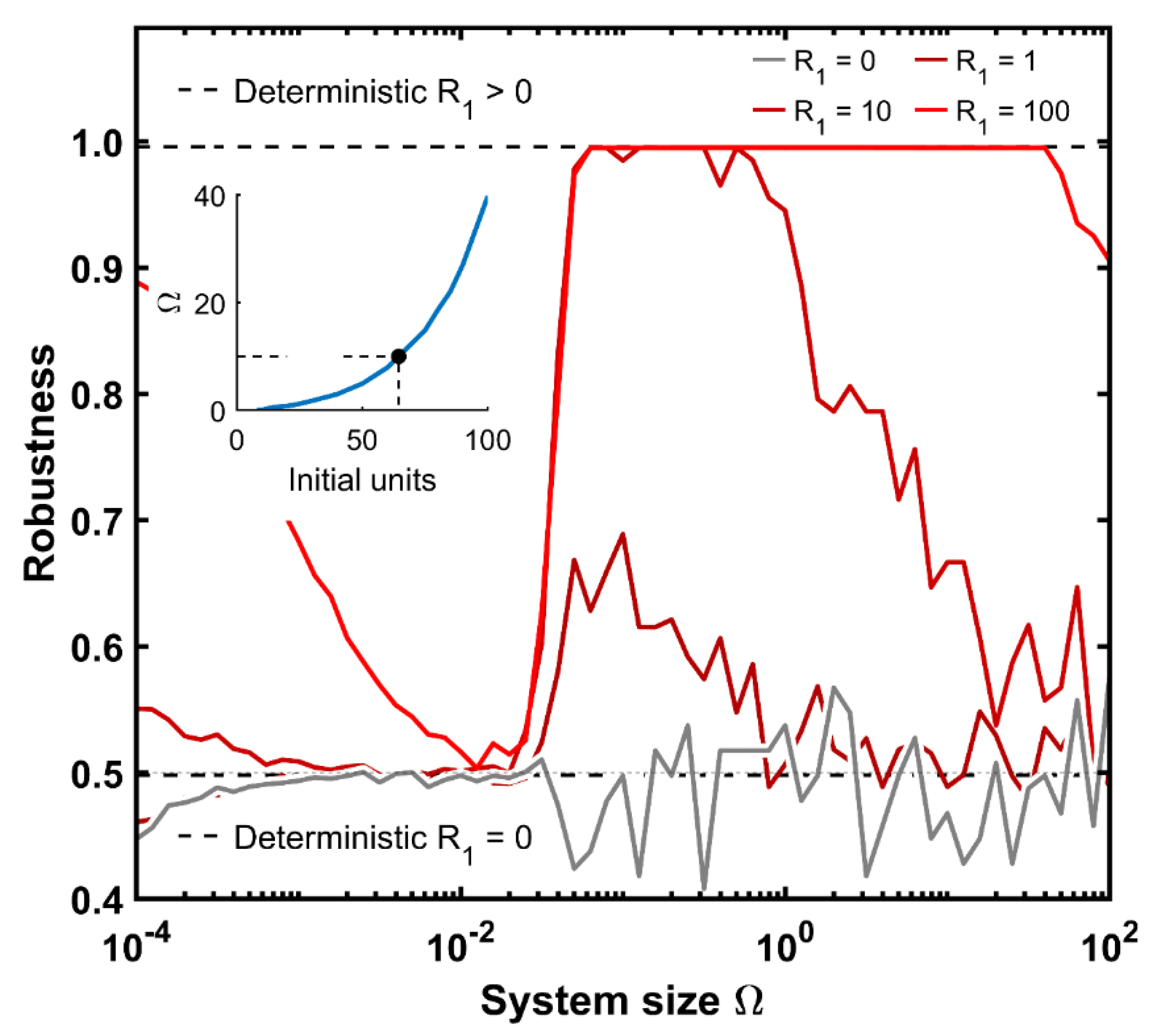
Remarkably, larger systems show a coherent operation starting from the R1 state. However, this is not the case for the smaller scales. Hence, it is interesting to delve deeper into the robustness of the machine as a function of its size and initial state information. For this purpose, we define the robustness of the system as the proportion of correct-type proteins (following the coherent design) for that semi-period with respect to the sum of all proteins for that time period. We calculate the robustness for the first two cycles, i.e., four periods, since the system behavior is the same for the following cycles.
Figure 6 displays the robustness of the system as a function of its size for a given initial protein amount, averaging 100 simulation replicates in each case. When the system departs from zero protein units (gray), the robustness is less than 0.5 for small cellular systems (around 0.45 for the smallest one) because the automaton is so chaotic that for some signal transitions, unexpected proteins can still appear: the signaling effect is too weak to prevent any type of protein from being produced, regardless of the signal correspondence at those time steps. Above sizes of 10
−3, the signal effect is already sufficiently strong to at least discriminate between both protein blocks (
Figure 5A, top graph). Therefore, the robustness oscillates around 0.5 for the remaining system sizes. Remarkably, the robustness value tends to have a greater variability for larger sizes. This occurs because the system has the same probability to start counting from green-R
3 than from the red-R
1 protein. This provides a robustness magnitude of either one or zero for each single run.
The next case is that with only a single protein of R1 as the initial condition (darker red color). The machine follows the same behavior as the previous case for values below 10−2. Above this threshold, the FSM can operate with robustness values slightly above 0.5. However, in larger systems, the machine output drops again to 0.5 because the system is too big for the initial information. A similar situation occurs with R1 equal to 10 and 100; robustness falls to 0.5 but in much higher cellular environments. Interestingly, any machine with a sufficiently large number of initial proteins, approximately at least 10 red proteins at the time of onset, reaches full effectiveness around an magnitude of 0.06 units. This cell scale roughly corresponds to 20 repressor molecules as maximal output within our parametrization set.
Moreover, the deterministic robustness has been outlined. Deterministic systems without any initial protein end up at a robustness of 0.5. The exact value is 0.498 due to minor protein units while one states dominates over the other. Similarly, any deterministic initial protein content above zero delivers a fully coherent FSM, with a robustness of 0.996, doubling the previous one as expected.
This value coincides with the maximal coherence of the stochastic simulations. Additionally, the inset plot of
Figure 6 illustrates the amount of repressor molecules at the onset of time that allows a maximal system size before the automaton starts to fail at being fully robust. This association seems to follow an exponential function: with a minor increase in the initial amount of proteins, the cell size can be much higher to retain full functionality.
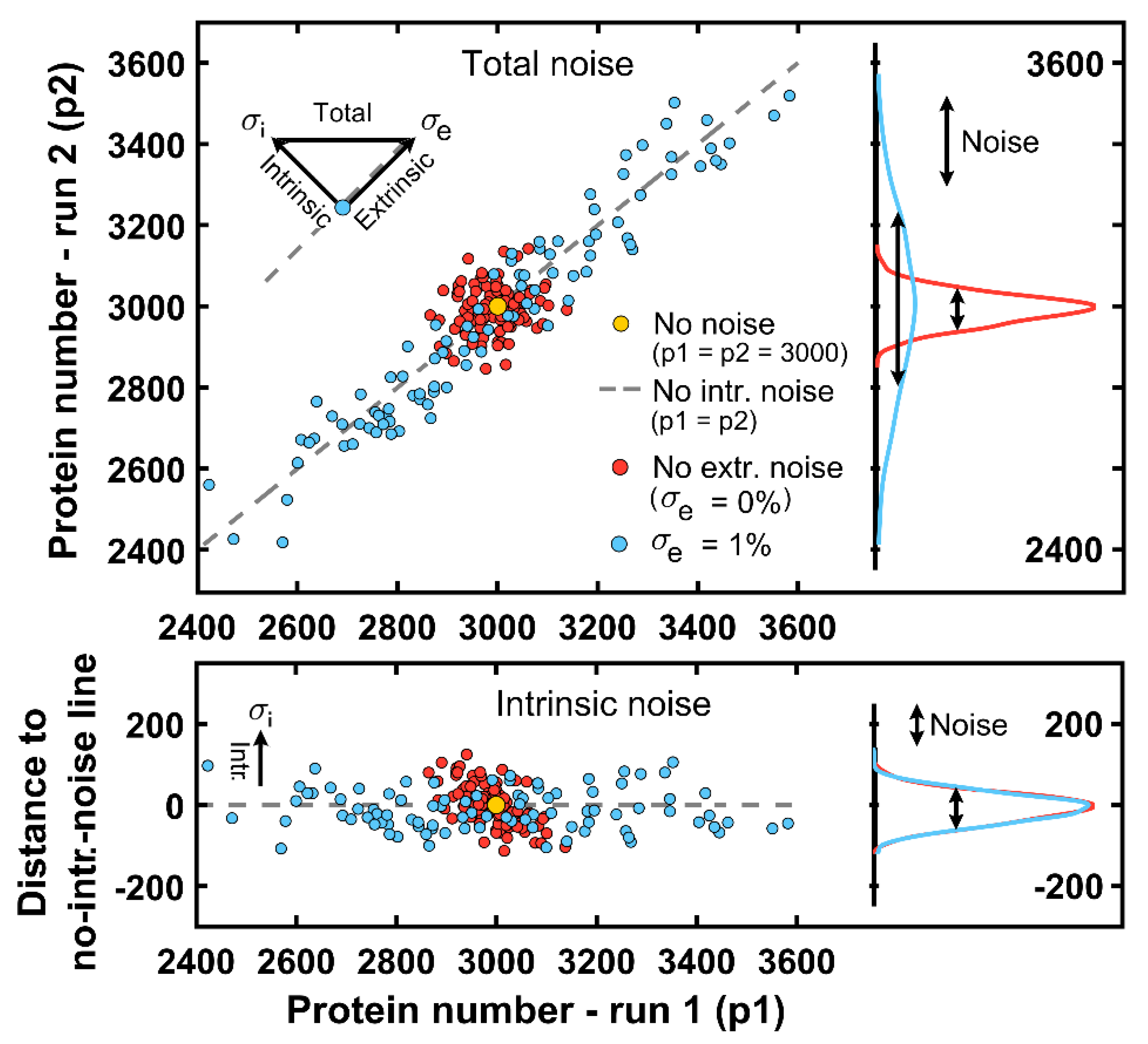
A related feature of the coherence of the device is the noise present in the cellular system. In this regard, intrinsic and extrinsic noises can considerably impact the machine’s performance; therefore, it is critical to assess their magnitude. For the case of a system size
of 10 (thousands of R
1 proteins per cell), the noise level is already low but still significant (
Figure 5B). To test the intrinsic noise of this system size, 100 cells were simulated with two runs for each (
Figure 7). For simplicity, the signal was set as constant and equal to
= 300. The R
1 initial protein amount was assumed to be 100 since it is sufficient for a coherent automaton, as
Figure 6 illustrates.
Intrinsic noise emerges from the inherent nature of living cells: systems with the same parameters can display different results when noise is present. Alternatively, extrinsic noise is an external stochastic process that affects molecular reactions in an equivalent manner. For the FSM, the extrinsic noise can be seen as a factor that promotes maximal protein levels to covary, and thus, it is orthogonal to the intrinsic magnitude (top panel of
Figure 7). Indeed,
Figure 7 displays two experiments: one without extrinsic noise (red dots) and the other with some extrinsic noise due to a 1% deviation from the mean value of the synthesis-rate parameter
(blue dots).
If one compares both cell groups, the total randomness, seen as a combination of intrinsic and extrinsic noises, is only enlarged due to the latter factor in the blue-cell group, while the intrinsic noise remains equal as the system size does. For the deterministic case without noise, both runs for the same cell (with the same
value) would result in a protein value always equal to
under steady-state conditions (yellow dot) while cells only displaying extrinsic noise would lie on the gray dashed line in
Figure 7 corresponding to no-intrinsic-noise cells (each run delivers the same protein amount, p1 = p2). In particular, the intrinsic deviation for most of the cells lies within ±5% of the mean protein amount (bottom panel of
Figure 7).
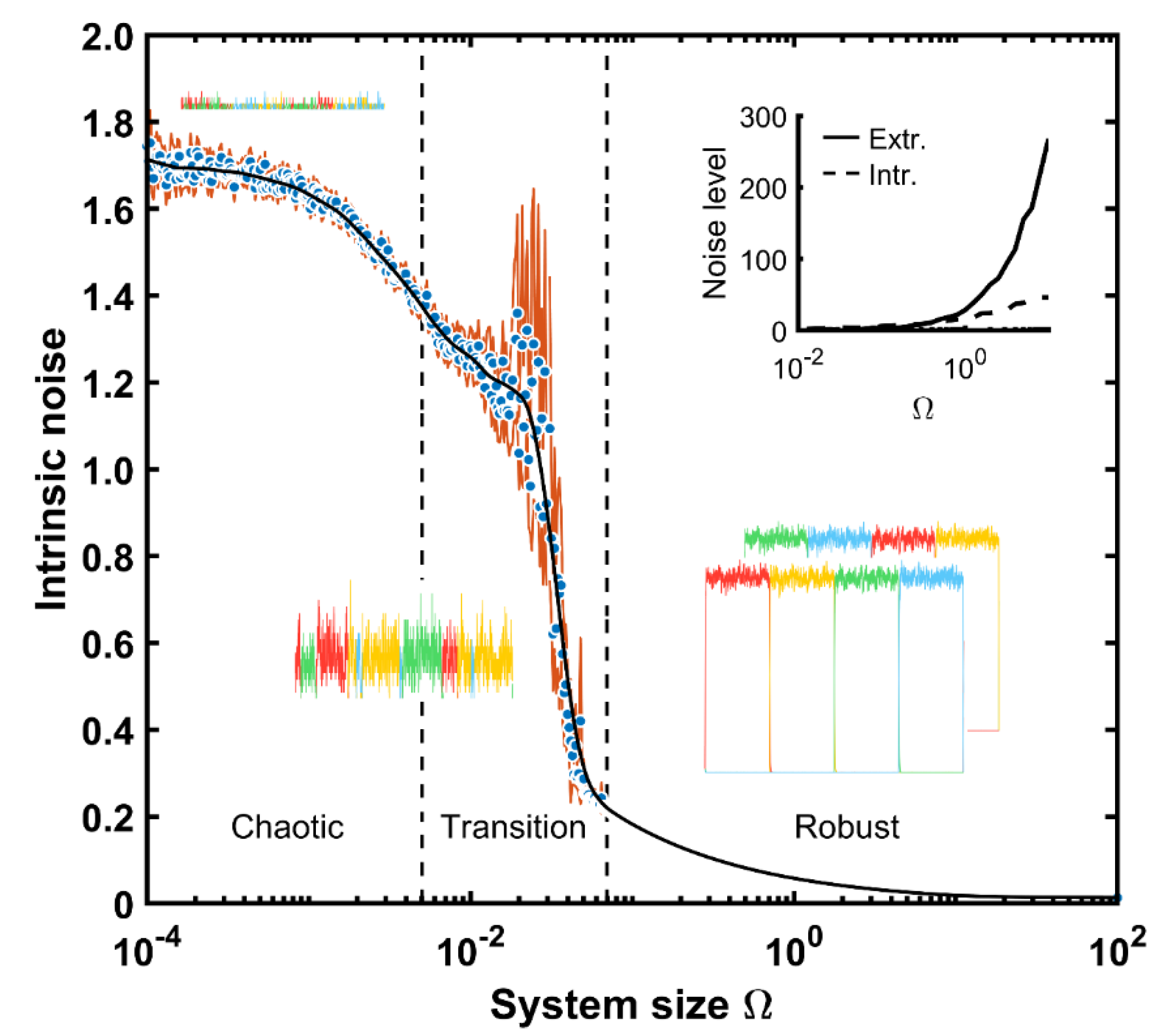
Once we have illustrated both noise types, we will estimate their magnitudes depending on the system size. In
Figure 8 the relationship of the intrinsic noise, given as the coefficient of variation for different cellular sizes, is depicted. The intrinsic noise is around 1.7 for the smallest systems and stays almost constant up to
values below 10
−3. For cells with more proteins, the system noise drops to 1.4 units. Interestingly, the confidence interval is rather narrow. This implies that the system is rather small and therefore, the possible amounts for proteins too (below 10 repressor units as a maximal amount,
Figure 5A). However, for
magnitudes between 10
−2 and 10
−1, the system displays a larger solution space where possible protein numbers increase so much that the protein means can be affected by high values, and the mean confidence interval increases. Alternatively, for magnitudes above 10
−1, the system is so big that the intrinsic noise given as the coefficient of variation remains low, below 0.2, and the confidence interval amplitude is almost zero. For larger sizes, the automaton works coherently if there is not enough initial information, but the system can start at the wrong state as already described in
Figure 6.
In summary, the system displays three different behaviors based upon its size. For very small scales, it operates in an almost random manner, showing up states that might not even be coherent with respect to the signal status. This chaotic performance is gradually transformed into a coherent device as the size increases. Indeed, there is a transition size band for
between 0.005 and 0.08 units, in which sustained states can be formed, but not for the whole semi-period. Under these conditions, the machine cannot shift the state in a sequential order. Above 0.1 units, the system displays a very low noise level, acting as a deterministic system (the confidence interval coincides with the mean and thus disappears visually), yet still depending on a sufficient amount of the initial protein content to retain the sequence in the appropriate order. The inset of
Figure 8 compares the magnitude between the intrinsic and extrinsic noise levels, assuming an extrinsic amount equal to the one in
Figure 7 (1% of
,
= 30).
The extrinsic level is lower than the intrinsic one for size values 0.5. Above this threshold, the system is so large that the extrinsic noise increases exponentially, representing almost 90% of the overall system noise for real-cell sizes (
= 1). It has to be noted that though the intrinsic noise is given in absolute units and increases with the system size (shown in the inset of
Figure 8), its coefficient of variation does not. The latter is given in relative units and decreases with larger system sizes as depicted in
Figure 8. This happens since in the latter case the noise is divided by its mean and this increases with the system size as shown in
Figure 5.
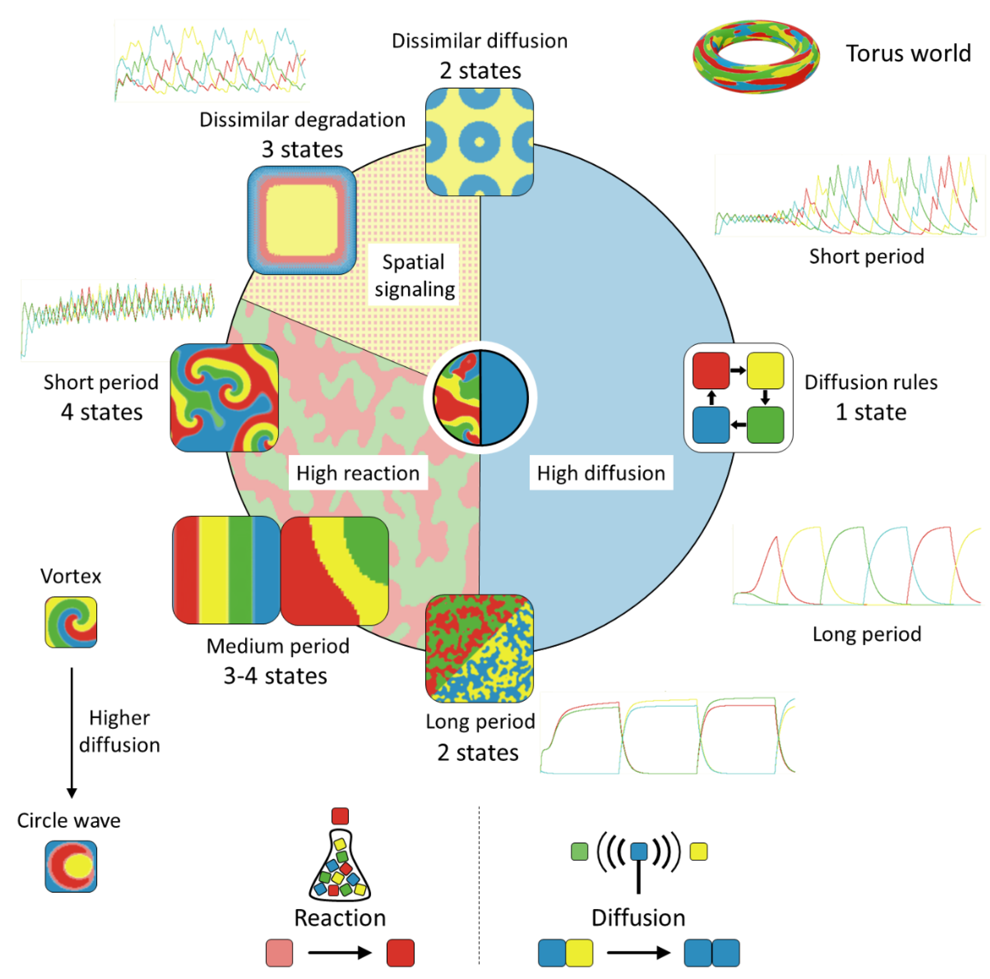
3.3. Spatial Model
For the cellular automaton formalism, we first studied the system with the same parameters as in the base case of the ODE set and chose a time step of 0.001 min and a diffusion coefficient of 0.01. In
Figure 9, different time steps for the CA simulation are shown. The world is composed of cells whose initial concentration of regulatory proteins is obtained from the uniform distribution [0, 2]. The protein with the highest concentration determines the patch color. This is for most cells shown in a pale tone due to similar concentration levels of all proteins in this random initialization. A few time steps after the signal appearance, only red and green cells remain due to the signal activation and repression of each protein block. However, once the signal vanishes, the concentration of red-green R
1-R
3 repressors is still so high because the signal period is rather long. This contributes to a delay in the manifestation of the other repressors (R
2–R
4), even in the absence of a signal. Progressively, both protein blocks tend to equalize their concentrations (we have assumed so far the same parametrization for each protein). The cells are decoupled from signaling but follow local state aggrupation. Further, diffusion contributes to the formation of larger clusters in which only one transcriptional factor dominates the others. Diffusion together with the rather long signal period is enough in this simulation to collapse the system so that after some time steps only a unique protein will be present (almost 100 times higher than any other). Thus, the CA of the FSM under the given parametrization set ends up as a single-color world of patches that can coherently shift within states following the signal inputs as required for a proper device design.
Different scenarios can be in silico tested by modifying boundary conditions and the parameter set. The main characteristics that will be checked are the impact of the signal period, the reaction and diffusion rate, and the degradation velocity of the regulatory proteins. We gave some flexibility to the system by opening borders, which permits us to observe more types of dynamics. In this way, the two-dimensional square lattice is equivalent to a torus as the neighborhood of the edge cells continues at the opposite border.
The FSM is a reaction–diffusion system in which both phenomena interact and create emergent patterns at a culture scale. The CA can be found in two basic situations, either the cells react homogeneously to external stimuli as a single reaction unit or local clusters appear. If diffusion rules, i.e., its rate is sufficient to absorb all the produced molecules, these are simply shared among all patches. In this case, mean properties do apply since there are thousands of replicates of the same cell. However, when reaction rules over diffusion, different cell configurations arise. Such figures might not be interesting when a synchronous and overall response of the culture is expected, yet can be useful when one seeks other behaviors, such as morphogenetic structures.
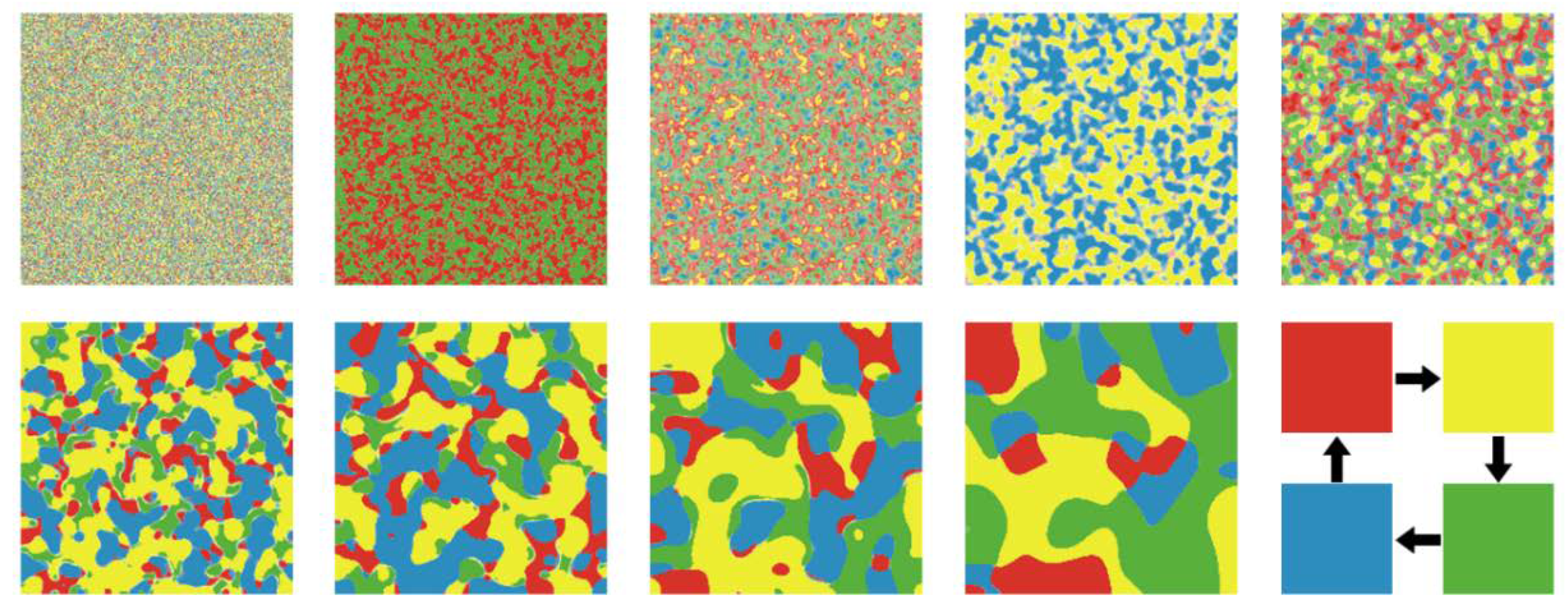
Figure 10 displays the automaton result of different cases after 100,000 steps in a torus world formed by 40,000 cells. Next to some of the simulation results, the time evolution of the four protein concentrations during the first 3000 steps is also displayed for a better illustration of the FSM behavior. The left side of the circle in
Figure 10 shows patterns in which reaction governs over diffusion, while the opposite happens on the right side. When diffusion rules, the other parameters are not relevant and the culture FSM shrinks to homogeneous behavior. Depending on the parameter set, the time needed for reaching system synchronization varies. Moreover, the signal period affects the response (right side of
Figure 10). Longer periods promote a steeper response and higher maximal protein content than shorter ones under the diffusion regime. The latter transiently create a chaotic behavior with multiple clusters reacting with each other that end up at a sole state for each time step.
Alternatively, when the reaction rate is sufficiently high (left side of
Figure 10), the system can retain bi-stable block activity. This implies that no single repressor is capable of reaching a concentration threshold to eliminate its partner protein (R
1–R
3 and R
2–R
4), and therefore, two states can coexist (bottom side of
Figure 10). Increased degradation rates
can lead to a single-color state since protein levels are reduced as well as the effective reaction rate. Similarly, if we increase the repressor capacity
, the automaton might again reach an attractor state where the diffusion phenomenon governs the whole system since the preponderant protein type can then inhibit the production of the rest.
A signal-period increase can promote differentiated attractors. For example, moving bands of same-state cells can develop. Further, if the period signal is rather short, vortices become visible (left side of
Figure 10). In each vortex center, the four concentrations are in similar amounts and a rotation pattern emerges, yet the vortex center does not move. Vortices remain as long as external perturbations are not strong enough to terminate them. This can only happen if stronger cell dynamics around the vortex absorb them, or by a sudden increase of reaction or diffusion rates. In the first case, the FSM ends up in two states, while in the latter, a round cluster can arise.
So far, it was assumed that if the external signal is a small molecule interacting with the transcriptional machinery of living cells, the stimulus is present or absent across the collection of functional units, i.e., the signal intensity is equal for all cells of the grid. However, we can also excite the system by applying optical or electrical signals at specific points. In this case, it would be interesting to analyze the propagation capacity of such stimuli within the culture and the pattern that appears due to the spatial arrangement of the signal input. For this purpose, we carried out several experiments in which the signal excites the system in specific cells but not in all of them (top and top-left side of
Figure 10). In general, keeping the symmetry of parameters, the spatial reduction of signaling contributes to the disappearance of the R
1 and R
3 states because they need signal input to actively produce their proteins.


