1. Introduction
The idea of STEM Education (Science, Technology, Engineering, and Mathematics disciplines) has been contemplated since the 1990s in the USA. Americans realized that their country predominant position may fall behind in the global economy and began to focus on promoting STEM education and careers [
1]. The emergence of STEM Education and the efforts made to promote it are not transforming into an increase in the number of students choosing STEM careers. On the contrary, students’ interest and motivation toward STEM learning has declined, especially in western countries and more prosperous Asian nations [
2].
In recent decades, STEM Education has evolved from a set of disciplines that were considered to be useful from a productive point of view to a new discipline that integrates the knowledge that makes them up. STEM learning is defined as the integration of a number of conceptual, procedural and attitudinal contents via a group of interdisciplinary skills for the application of ideas or the solving of problems in real contexts [
3]. While it is widely acknowledged that mathematics underpins all other STEM disciplines, there is clear evidence that it plays an understated role in integrated STEM education [
4]. We agree with the author in [
5] that the most relevant role mathematics should have in STEM integration is through mathematical modelling as a vehicle to connect the contents and methods of STEM disciplines with real-world problem solving.
One of the STEM cross-cutting topics that has received the most interest is computer science, because of its relevance in solving real-world problems. Computer programming is an aspect of computational thinking and it has globally become a focus of many school curricula over the last 10 years, with the intent that students develop and demonstrate computational skills [
6], higher-order thinking skills, and algorithmic problem-solving skills [
7]. Educational research has shown great interest in studies on early learning programming, but efforts still need to be directed toward the full development of programming skills for the various STEM careers. The difficulties faced by students in higher levels of engineering or scientific careers when dealing with computer problems in their own disciplines can provide future students with a demotivating image that influences the low choice of these studies. It is necessary to connect computer learning with real problems that can be solved and find methodologies that adequately accompany the work of students.
College students in engineering or science, and especially those that are enrolled in computer science-related degrees, need to learn how to analyze and design algorithmic solutions to computable problems beyond the mere construction of programs. Generally, the way to teach the different algorithmic techniques was based on the presentation of basic problem-solving techniques applied to some classical examples. From here, students were left with a collection of problems to solve without having room to do an in-depth analysis of these techniques once they have been programmed. This way of approaching the teaching of these techniques did not usually include elements of reflection on the consequences of the design made. Consequently, rather than training programmers, coders were trained without the ability to understand a problem to plan and design an algorithmic solution that was then coded [
8]. To overcome these drawbacks, in recent decades, efforts have been made with approaches, such as Problem-Based Learning (PBL) [
9] or Inquiry-Based Learning [
10].
In this article, we present the design of a sequence of activities that aimed to promote learning on analysis and design of algorithms in Engineering Studies. This sequence of activities is oriented to students in the third/fourth year of Computer Engineering degree, and second year of Data Engineering and Computational Mathematics degrees. The didactic design is based on the principles of mathematical modelling as a PBL approach. The Salesperson problem is chosen as a real problem to work with, because of the range of existing algorithmic approaches to solving it. We develop a didactic software tool, named Graph-based Problem Explorer (GbPExplorer), which allows graphal visualization and algorithm techniques coding in order to support students learning. In this way, students can develop their skills not only as programmers, but also as analyzers and problem solvers.
The remainder of the paper is structured, as follows.
Section 2 presents the theoretical foundations of the proposal. In
Section 3, the educational context is detailed.
Section 4 is devoted to explain the process of designing and refining of the project.
Section 5 and
Section 6 detail the elements of GbPExplorer and the project sequence development. Finally,
Section 7 discusses the identified didactic potentialities and concludes the paper.
2. Theoretical Framework: Modelling in Education as Problem Based Learning Approach
In recent years, there has been increasing interest in introducing new activities that include modelling processes in the curricula of different educational levels due to their didactic potential for connecting reality with mathematical content [
11]. This interest is due to the evidence of the usefulness of modelling in all scientific disciplines, as modelling has been shown to be one of the most powerful tools for scientific purposes. If we focus on modelling in educational settings, Lesh and Harel [
12] define mathematical models as “conceptual systems that generally tend to be expressed using a variety of interacting representational media”. Their purposes are to construct, describe, or explain other systems while using concepts and accompanying procedures.
The way that students create mathematical models to solve problems is currently under study, with different points of view [
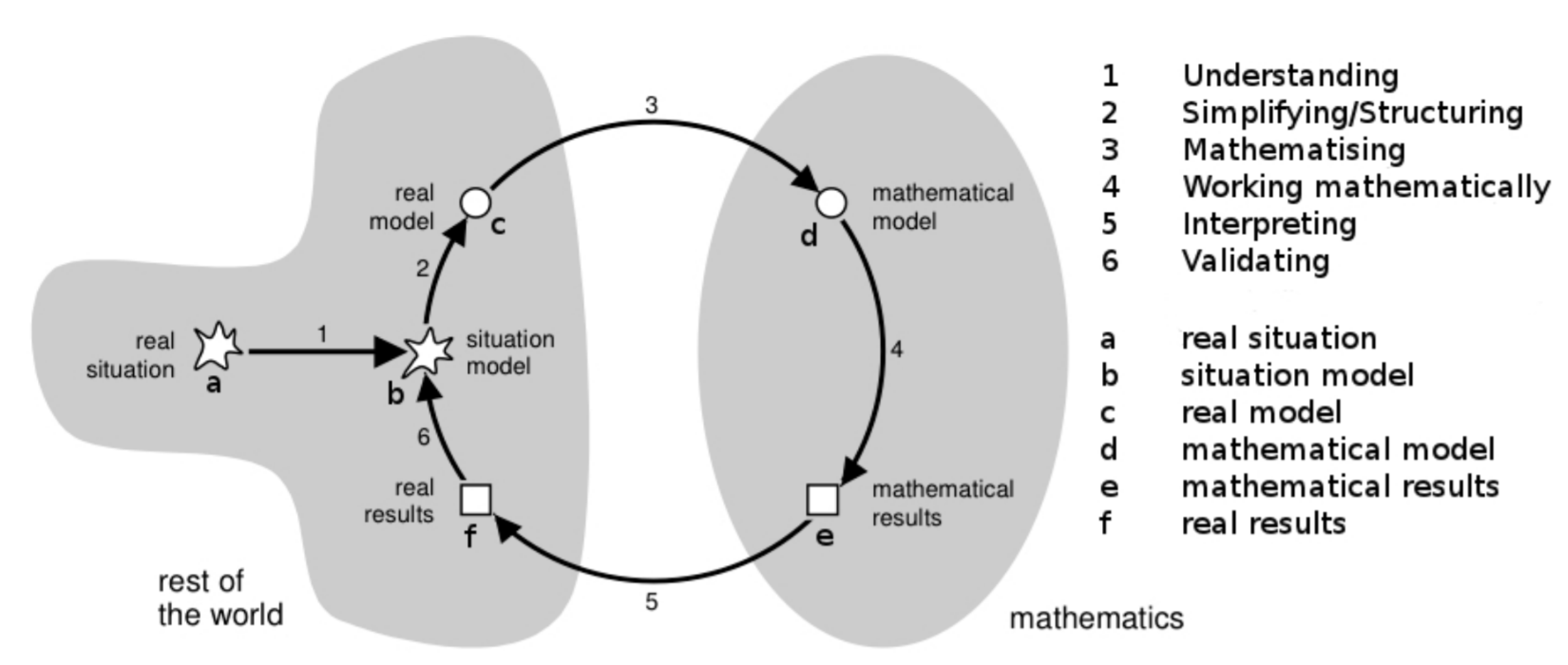
13]. It is generally accepted in the literature that modelling processes are cyclic in nature [
14], as shown in
Figure 1. During the resolution process, students try to solve problems by going through different stages and then going back to reassess the studied situation. Therefore, the process is repeated in different cycles, in which students improve the models and solutions found for the problem they are working on, adapting them to the requirements of the problem statement [
15].
However, the didactic uses of modelling go beyond the modelling process itself and can be used as a vehicle for teaching other content in educational environments [
16,
17,
18]. An alternative way of using modelling is to propose a real problem in its context and provide a concrete mathematization of that problem. In this way, students work in the abstract domain and can learn new knowledge from experimenting in this simulated situation, taking advantage of the information provided by their knowledge of the real phenomenon.
If we focus on computer-based learning, in recent years there has been a great deal of interest in changing engineering teaching methodologies [
19,
20], due to changes, both in the skills that are required for future engineers [
21] and in the entry profile of students [
19,
22]. Among these methodological innovations, those that seek to actively involve the student in his/her learning process, achieving positive results, particularly in the understanding of concepts and in the ability to solve problems, have been highlighted [
23,
24]. In these proposals, we find the Problem Based Learning (PBL), as a recurrent strategy for engineering education [
25]. There is an extensive literature on the basis and pedagogical foundations of PBL [
26,
27] and, given its popularity in recent years, it has generated a large amount of research on teaching in several areas of knowledge [
28] and has been refined with further contributions from research and practice [
29]. PBL was first used in 1980 in medical education [
30] and, since then, it has not only spread to all areas of knowledge, but some universities, such as Aalborg University [
31], even use it in all of their degrees.
In the fields of engineering and science, knowledge requires study and learning according to hierarchical dependencies that follow strict regulation [
32], both at the micro level, i.e., thematic units within courses, and at the macro level, in relation to the units that exist between courses and the curriculum. The teaching of computer programming and algorithm design has become very relevant in the current context of engineering education, given the massive availability of computer resources and tools that can be used in practically all sub-disciplines, and the great potential of computer tools to help engineers to solve the problems of increasing complexity and sophistication. In computation courses, engineering students must develop a set of cognitive and meta-cognitive skills aimed at solving problems through computer thinking and programming [
33]. Learning computer programming and algorithm design is similar to learning knowledge of other areas of engineering and sciences, because programming must be learned according to the hierarchical order of knowledge and skills needed. The learning process involves the continuous exercise of factual knowledge, such as lexemes, keywords, and the valid grammatical constructions of the programming structures, as well as also conceptual knowledge needed to build in-depth representations [
34]. This includes the representation of data while using variables, the construction of decision, iteration and recursion structures, the use of structured data, and the definition of functions. In addition, problem-solving through computer programming involves the development of superior thinking skills, mostly analytical and creative, including the breakdown of complex problems in sub-problems, the design of algorithms to solve them, and the ability to effectively translate the internal representations of algorithms into valid syntactic and semantic code in a programming language. The students become more adept at programming, as they acquire and effectively articulate all of this knowledge, and build their own reusable schematizations to more efficiently address new problems [
32].
Problem-based learning (PBL) is a student-centred pedagogical approach in which students learn about a topic through the experience of solving open problems [
35]. The problem-based learning process does not focus on problem-solving from a single solution, but it allows for the development of skills and attributes that are desirable in students. These include knowledge acquisition, communication, and collaboration within a group and interaction between students. PBL proposes an open and poorly structured problem to the students and provides them with concrete questions and materials that allow them to adequately develop the activity in order to promote these learnings.
When introducing PBL in different engineering subjects, it has been shown that it is necessary to introduce specific supports to promote certain types of activities or interactions between students [
36]. In the case presented in this article, and to facilitate the interaction of the students in the key aspects of the project while allowing the proposed learning, the work is done through the use of a specific software tool. The tool that we present provides students with a concrete representation of the problem studied and a programming environment, so that they can experiment with it. If we focus on programming learning, modelling provides a context in which to test and validate the solutions that were developed by students going through the different solving stages. In this way, an environment in which students can experiment with a given model of a complex reality allows them to analyse the relevant aspects of the different programming techniques that can be used in the resolution.
3. Educational Context
As we explained above, we propose a project for coding and analyzing several algorithms in accordance with the objectives of the subject “Analysis and Design of Algorithms”. The aim of this subject is to provide students with advanced programming knowledge and introduce them different styles and paradigms of algorithm design. The main objective is that students develop skills in algorithm design and analysis in order to be able to solve real-world problems effectively and efficiently according to the requirements established by a potential client. Topics in this subject include the formal specification and verification of problems and programs, computational complexity, and algorithmic techniques, such as greedy, backtracking, branch and bound, dynamic programming and probabilistic methods. Examples of real problems that can be addressed by these techniques are: tasks/stocks/schedule/costs/paths planning optimization, automatic text correction, signature authentication, financial decision maker, error recovering in information transmission, and natural language recognition.
The project presented here proposes the resolution of a classic problem, the travelling salesperson problem, by three of the algorithm techniques, as well as some variants, and a computational complexity analysis in order to extract the essence of the main objective of the course, which also involves an analysis of the algorithms. The original travelling salesperson problem [
37] is a very classic optimization problem that has been studied along decades. Its relevance is recorded as early as the 19th century and its first mathematical approach dates back to the 1930s and it responds to the following question:
Given a set of cities and the distances between them, which is the shortest path that visits each city (or a subset) and only once?
Although the problem is computationally complex (it is an NP-hard problem), a large number of heuristics and exact methods are known, so that some instances from hundreds to thousands of cities can be solved. Additionally, it has several applications in different fields, such as planning, logistics, electronic circuits, or as a subproblem in DNA sequencing. In those cases, cities are replaced by the object of interest (clients, DNA extracts, etc). Notice that the problem can be represented by a graph. Each vertex corresponds to a location joint by an edge with a known length.
Regarding the specific algorithmic techniques to be developed in the project, we consider the following ones and some variants:
Greedy. These kind of algorithms build a solution to the problem in successive stages, always trying to make the optimal decision for each stage, without taking further consequences into account. It is a very simple method that can be applied to numerous problems, especially for optimization ones. The drawback is that they not always produce optimal solutions.
Backtracking. These kind of algorithms compute an exhaustive search among solution space. That is, it builds the solution in successive stages, choosing an option among all the remaining possibilities each time and maintaining the chance of undoing the last decision taken. It is an exhaustive and, thus, tedious and time-consuming algorithm, but it takes the advantage that can compute all the solutions and, depending on the problem, can be posed to speed its computation.
Branch and bound. This method is a variation of the design of backtracking and it is usually used to solve optimization problems. Both of the techniques build an incremental solution by checking the constraints of the problem at each partial solution but, while backtracking works with a unique solution at a time, branch, and bound works with several partial solutions at once. Besides, backtracking leads a priority depth search, while branch and bound decide the best solution to follow up by means of a heuristic.
From the perspective of students, it is difficult to connect the specific characteristics and needs of real-world problems with the algorithmic techniques that are designed to solve them. The classic teaching strategy usually presents the techniques accurately in the classroom using typical examples and leaves time for students to make the necessary connections autonomously. This does not ensure that students develop the necessary skills to be able to deal with all the processes of solving a problem. It is from this perspective that PBL is taken as a way of articulating activities.
To this end, a practice module that is based on project work is introduced to promote this development of problem-solving skills based on a real problem. The project is accompanied by a specific software tool that allows for work on the key aspects of the problem approach and its resolution. The tool makes possible to visualize the data structures used, to develop code modules that implement different types of solutions and compare them in order to assess their suitability and to develop studies of algorithmic complexity. This provides students with a space to explore and self-validate their own coding of solutions.
4. Project Design Methodology
In this section, we explain the design process that is based on an educational design research [
38] for the refinement of the project through several iterations until the construction of a tool and a didactic proposal with the didactic objectives explained above.
As we explained above, after taking the subject “Analysis and Design of Algorithms” students are expected to be able to deal with real-world problems from an effectiveness and efficient codable point of view. In particular, they will develop skills to analyze algorithms, compare between them, and determine which ones solve a given problem in an optimal way, while taking into account the intrinsic efficiency and/or accuracy requirements of each environment. Besides, during the first academic years (2015–2016, 2016–2017, and 2017–2018), we gave the subject in Computer Engineering Degree, it was structured as sessions of theory (one session of 2 h per week), problem-solving (one session of 1 h per week), and lab work (one session of 2 h twice a month).
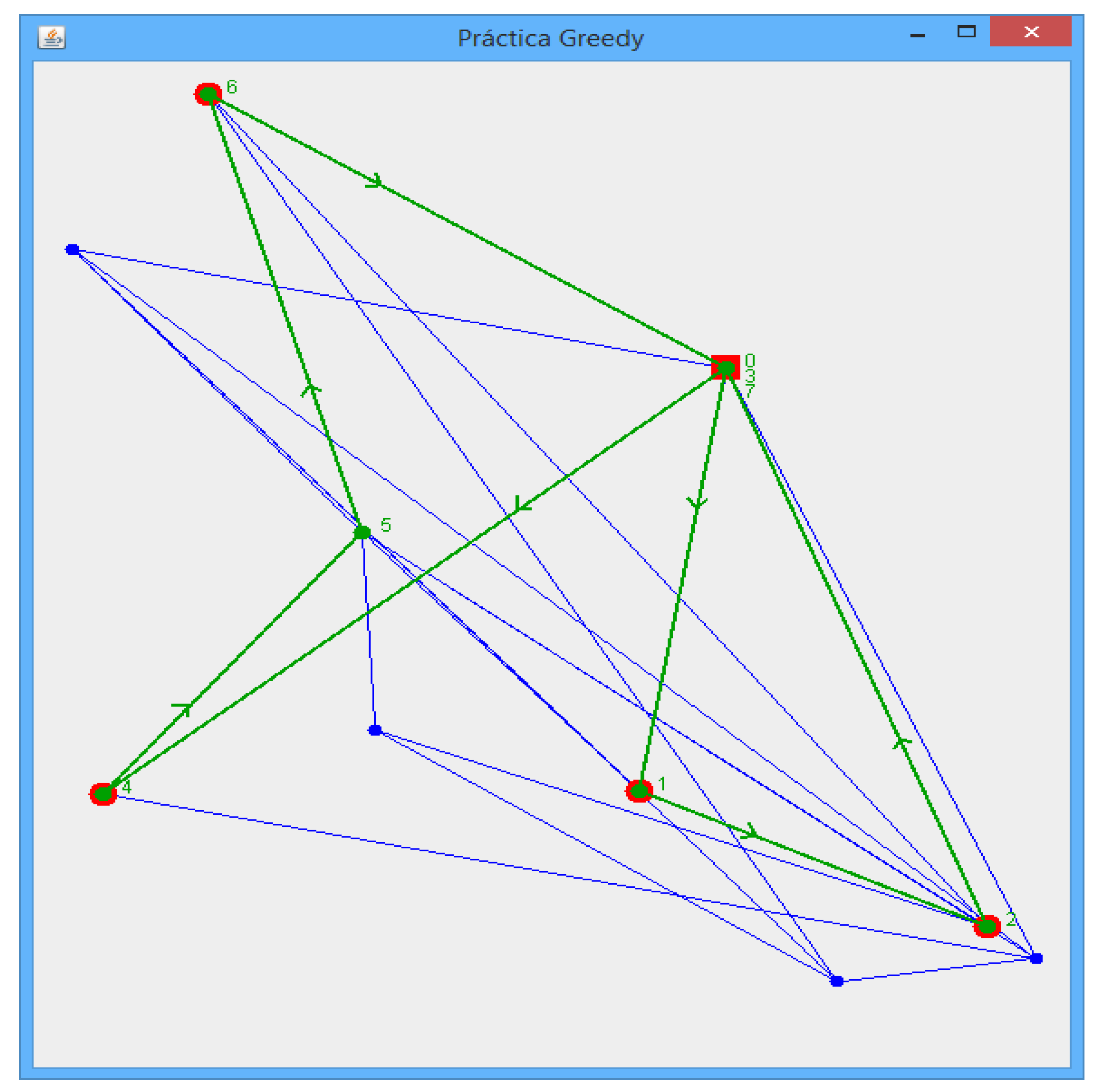
Keeping that in mind, in the 2015–2016 academic course, we designed a practical project to be developed during the lab work sessions, with the support of the teacher, and also autonomously by the students. During that course, the structure was, as follows: in the first lab work session, we presented the project as the aim to be developed during the following five sessions in parallel with the explanations of the algorithmic techniques that were performed in the theoretical sessions. That is, we presented the aim of the project, the planned development, a very naive software tool (i.e., a preliminary version of the current tool GbPExplorer), to be used as a crutch, and the evaluation process of the project. Regarding the tool, we simply provided the students with a graphical interface together with its corresponding code. The students had to code from scratch the scripts related to each algorithmic technique and call the interface by their own in a command line. An example of such a graphical interface, which was coded in Java, is shown in
Figure 2. Subsequently, the students became familiar with the code and data structures to be used and we let on their own to develop the project during the following sessions.
During the first year, we detected several shortcomings that can be summarized in two main points: (1) students needed closer and more continuous support from teachers and (2) students needed more feedback on the results that were obtained by their codes. Consequently, in the next two academic years (2016–2017 and 2017–2018), we iteratively refined the sequence of project activities along with the sessions. For example, we introduced a specific follow up of students in the middle of the project to give and get feedback on the evolution of the project. We also realised that an automatic corrector was needed for providing immediate feedback. However, we still identified other weakness, such as a good basis for problem comprehension, proactivity in creating their own test datasets to find algorithm failures, or programming gaps carried over from previous courses. This observation of the students’ needs to develop the project successfully led us to introduce changes from two different perspectives, in the concreteness of the activities, and in the form of the software tool that supports the work.
We resort to mathematical modelling framework [
14,
15] as a PBL approach [
26,
27] and planned our global project following the modelling cycle that is described in
Figure 1. At the same time, an innovation group proposed introducing a structural change in the methodologies to promote active learning in Engineering Studies [
39], so we proposed an organizational change in some subjects. From the academic year 2018–2019 in Computer Engineering and directly from the creation of Degrees in Computational Mathematics and Data Engineering, this subject is structured in 25 sessions of 2 h in 14 weeks. We combine several active methodologies to work on different algorithmic techniques as well as other topics, such as formalisation of problems and scripts and computational and algorithms complexity. Six of these sessions are exclusively devoted to the project development in the classroom.
From the perspective of the software tool that supports the work of the students, we redesigned it to integrate all of the elements necessary to deal with the handling of the graphs structure, visualization, algorithmic techniques coding, and problem-solving evaluation. This new tool allows for students not only to work directly on the relevant aspects of problem-solving, but also to avoid collateral difficulties that are caused by the fragmentation of the different programming modules to be used. In
Section 5, we present the current interactive tool, while, in
Section 6, we detail the way that we combine the agents involved in the tool in the learning sequence.
5. The Graph-Based Problem Explorer
In this section, we present the GbPExplorer, which is the software that acts as the main vehicle to experiment with the problem-solving in this project. GbPExplorer is hosted in the following open access repository:
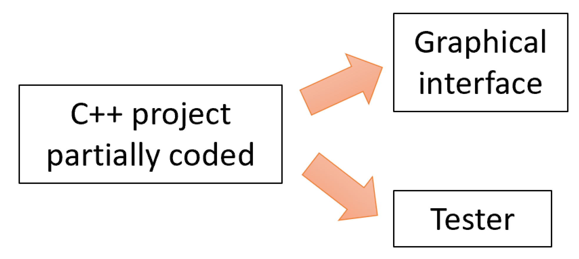
http://www.cvc.uab.es/people/javier/GraphApplication/GraphApplication.html. It can be mainly split in three different components, as we show in
Figure 3: (1) a solution in C++ partially coded where students have to code the solving algorithms by different paradigms; (2) a graphical interface that allows to pose different situations of the problem (that is different graphs), and check the correctness of their solutions; and, (3) testing executable files that serve to analyse and compare the performances of their solutions.
5.1. C++ Project
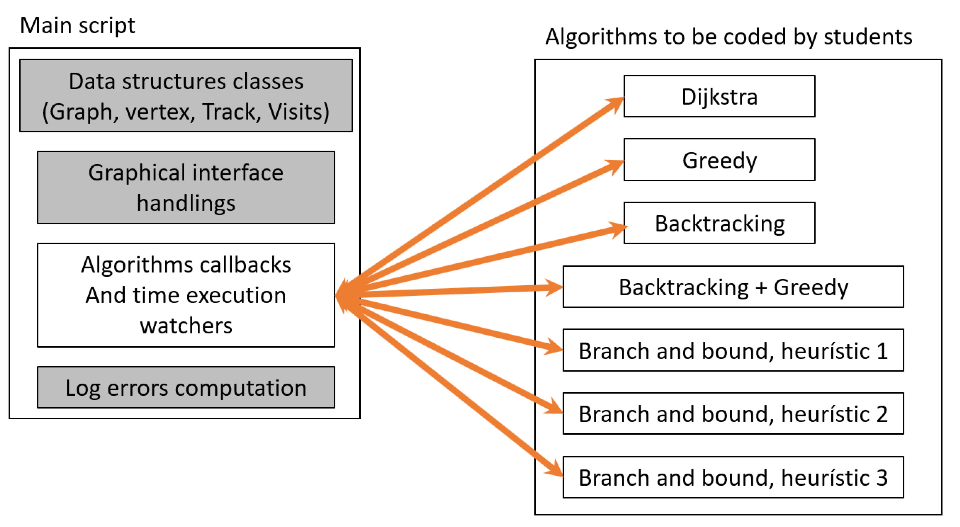
The students are provided with a partially coded C++ solution. This solution contains the code of the graphical interface, the shell of the solution to the travelling salesman problem (i.e., the main structures needed to solve the problem and all the callbacks to the scripts of algorithmic techniques) and a log with the computation errors. In addition, the students are provided with a report with the technical documentation of the solution. We sketch the idea of the solution in
Figure 4.
Grey boxes are already coded but are visible for better understanding.
Listing 1 shows an example of part of the code.
In the technical documentation, the code is also shown together with an explanation of each code cell, like the following:
CVertex class represents a vertex in the graph. This class contains the point on the Euclidean plane where the vertex is and a list of its neighbors. Additionally, it contains the fields m_DijkstraDistance and m_DijkstraVisit, which are necessary for coding Dijkstra algorithm.
The white boxes in
Figure 4 correspond to files that need to be coded by students. In
Listing 2, we show an example of the code given before implementing the solution.
This C++ solution serves to standardize the constraints that are necessary to adapt the activities to the particular aims of the subject. This means that students receive clear milestones during the project, while being given the freedom to code the algorithms (which are the objectives of the subject).
5.2. Graphical Interface
The interactive graphical interface contains several modules that serve to pose different problem situations (i.e., different graphs) and check the correctness of their solutions. That is, it allows for the generation of random graphs and also specifically designed ones, both with different number of vertices, edges, and vertices to visit. This allows for creating realistic representations of graphs, inducing students to retain the knowledge and skills about graphs that will later be applied in cases where this representation is useless.
Besides, once students code each algorithm, they can visually check the correctness of their solutions in two different ways. On the one hand, they can display the output of their algorithm and manually reconstruct the track to check whether the algorithm builds the solution in the expected order. On the other hand, they can test their algorithms with a dataset of 10 different graphs that were already prepared and given by the teaching staff. This dataset contains a set of graphs with their corresponding visits, distances between points, and optimal tracks. The students can load a particular graph from this dataset and compare the output that they obtained with the tracks. Both ways of testing serve to provide students with their own immediate feedback.
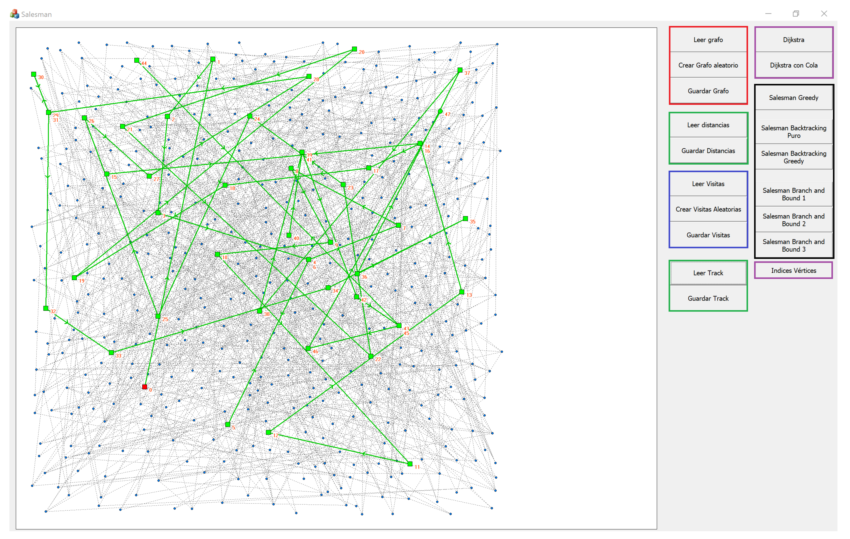
Figure 5 shows a view of the interface. On the left side, there is the visualization of a particular graph, while, on the right side, there are several modules that provide a set of utilities to explore the different necessary aspects to work in each phase of the project. These utilities can be split in five different categories: graph handling, visits handling, solution handling, algorithmic techniques, and intermediate utilities.
Graph handling (red box): this module allows for creating a graph, either reading it from a file, or creating a random graph with a fixed number of edges and vertices decided by the user, and save the last created graph.
Visits handling (blue box): this module allows for defining the locations to visit, either reading them from a file or creating them randomly, and to save the last ones.
Solution handling (black box): buttons in this module are the ones that students have to code to solve the problem in the different paradigms.
Algorithmic techniques (purple box): buttons in this module are codable utilities for visualizing their intermediate results.
Intermediate utilities (green box): this module allows for reading a solution from a file and save a new solution concerning neither techniques (track) or intermediate utilities (distances).
5.3. Testers
Finally, the GbPExplorer offers students another type of support, which is aimed at checking their outputs on the given dataset from an analytical point of view, with two aims: (1) to check exactly at what point their algorithm fails and (2) to check their execution times and obtain feedback on the efficiency of their code. This computation times will later serve students to set up the experiments for algorithm comparison analysis.
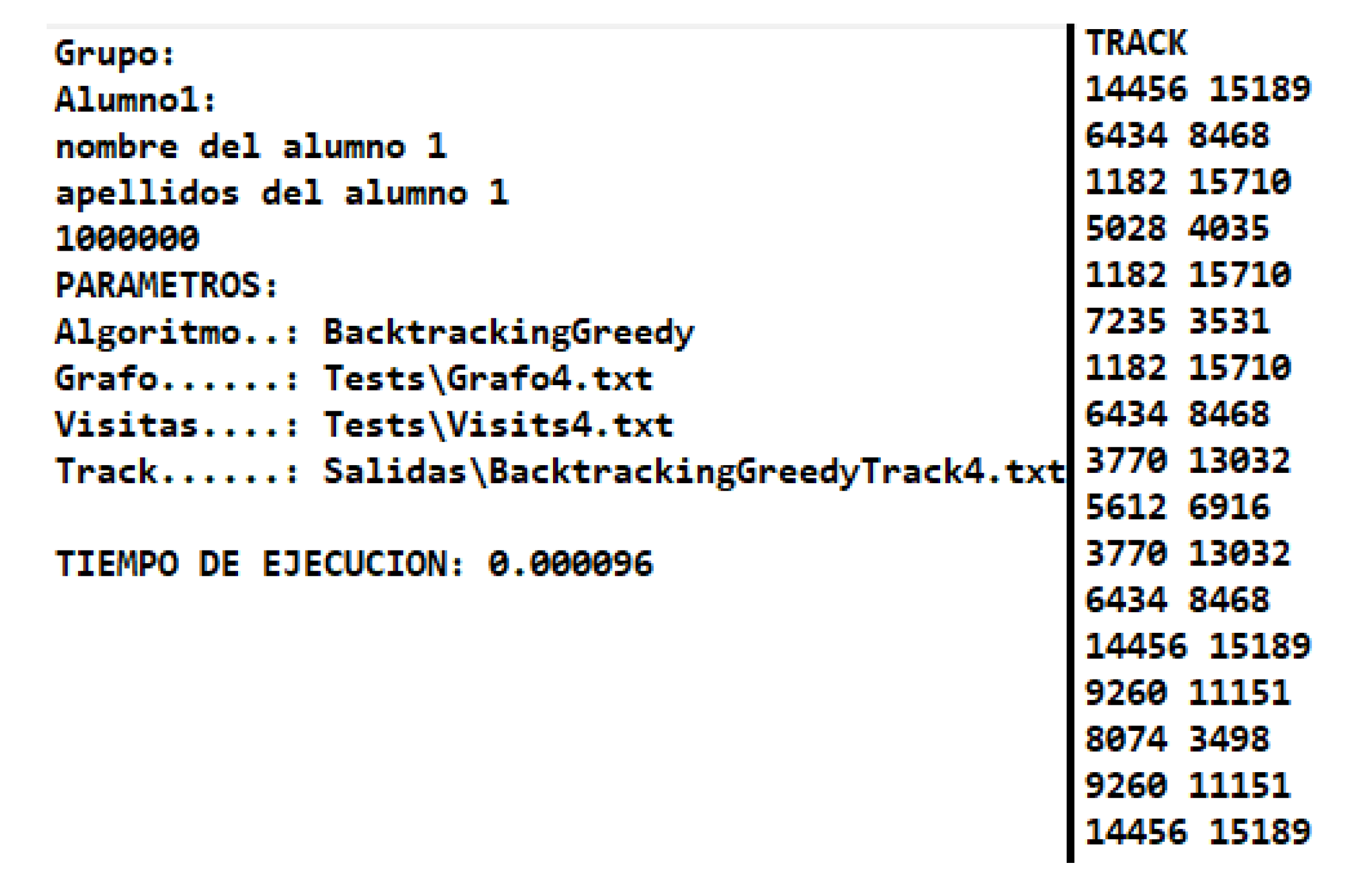
The outputs of these testers are presented in several text files, all of which are automatically generated and saved in a new folder by a corrector. On the one hand, for each graph and algorithm, students obtain a file with the student and parameters data and runtime and another file with the track obtained by the student’s algorithm.
Figure 6 shows an example of the text files that were obtained for the graph number 4 and the algorithm Backtracking + Greedy. On the right side, we can observe the track obtained by a student.
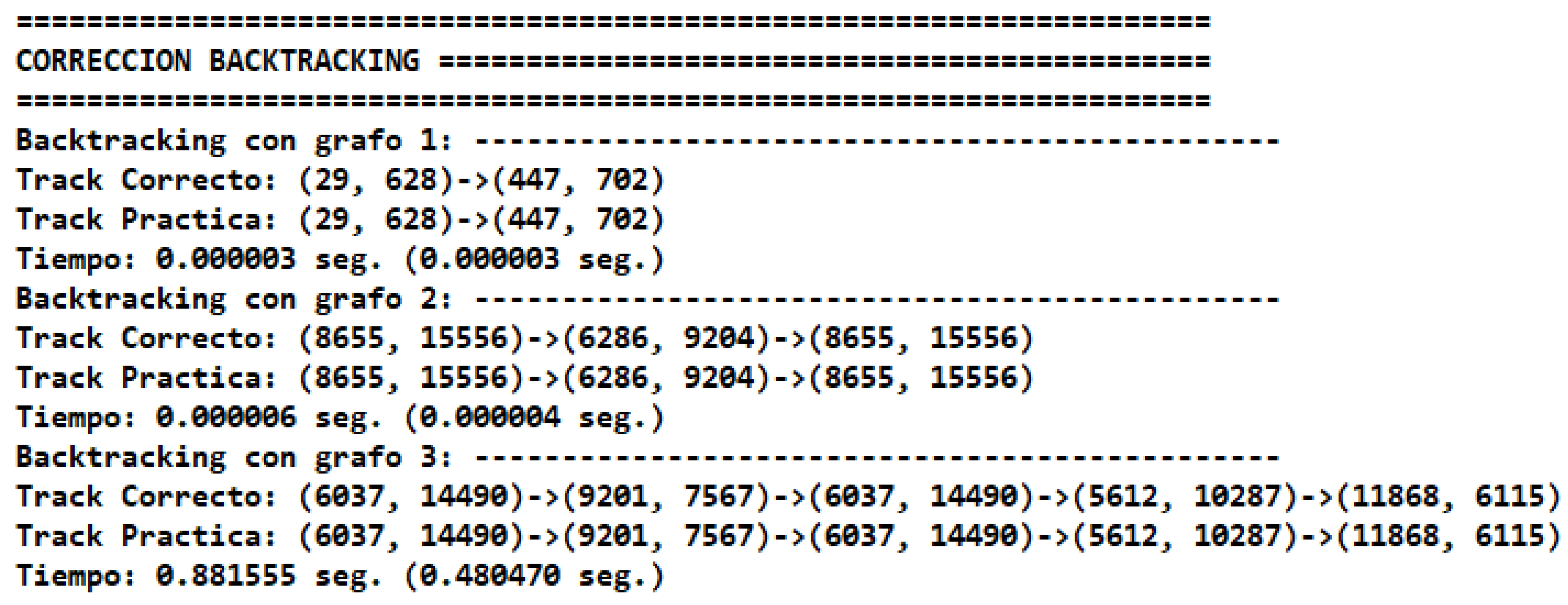
On the other hand, the students also obtain a summary of the results for the whole graph dataset and all the algorithms. With this file they can compare their output with the expected results. In case they obtain an error, there is a message with an explanation as we will show in the next section.
Figure 7 shows a brief extract of the file that was obtained by a student.
6. Project Sequence Development
In this section, we present the didactic sequencing of the project. Given that the purpose is to promote learning of the various processes associated with salesperson problem solving, this project is split in several activities throughout the course covering the modelling cycle [
14] presented in
Figure 1. In a real modelling process, the solvers work through the different phases until they generate a solution that they validate in the real world and, if it does not fit the needs of the problem, they restart a new modelling cycle. In the project, this behaviour is adapted and adjusted by proposing concrete activities that allow students to advance between stages through the modelling phases.
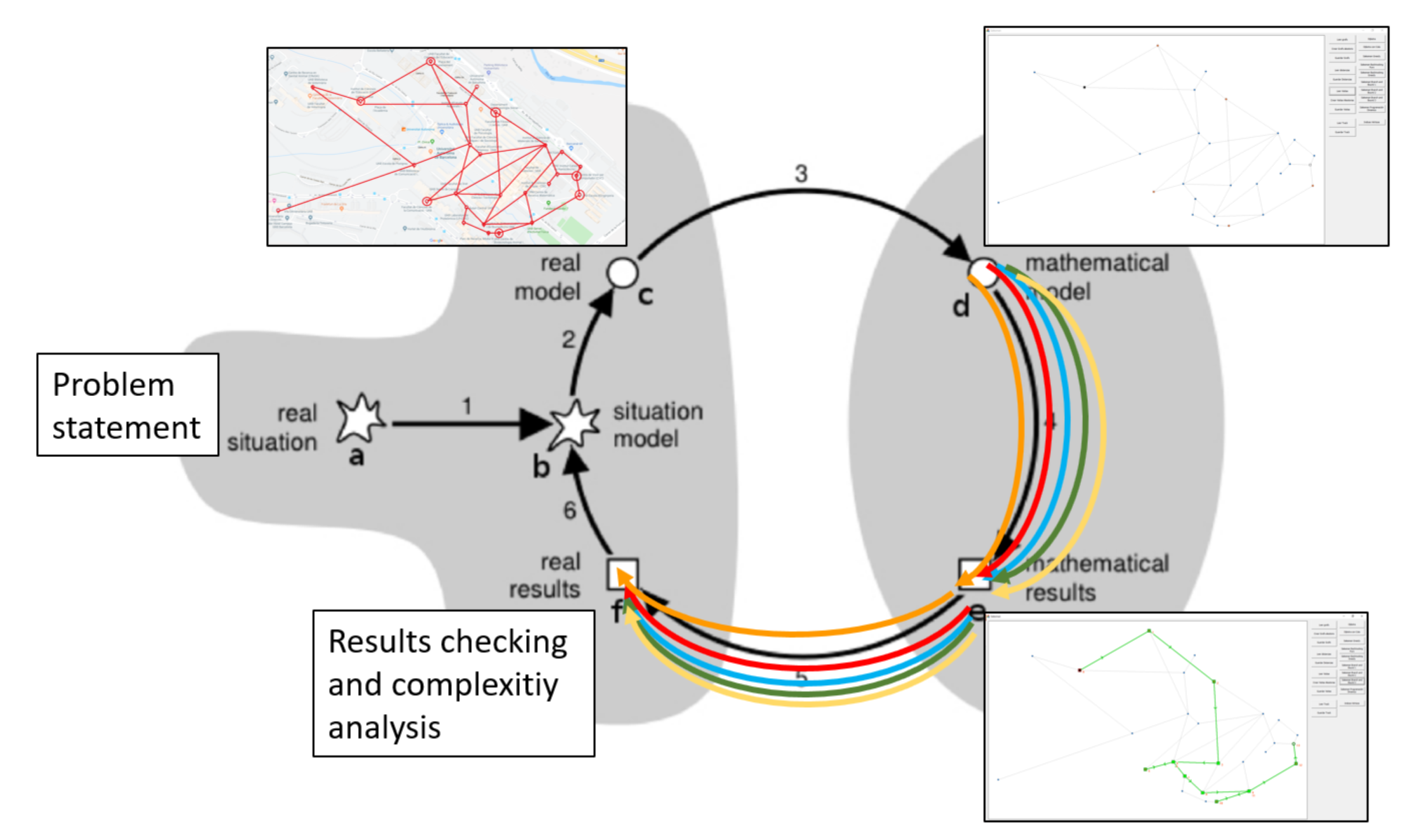
Figure 8 summarizes the activities that were introduced in each one of the modelling stages.
Specifically, the sequence of activities begins with: (a) a presentation of the problem statement, and a discussion promoted to determine (b) the situation model of each of the students and agree (c) the real model to work on. This initial modelling process allows for the transition to mathematical and computer work using the GbPExplorer. In (d), the mathematical model is implemented to work on the software tool. Each of the possible resolution techniques is implemented to generate (e) mathematical results that are (f) validated and checked for each of the techniques, allowing a comparison of methods from the point of view of computational complexity. All of the steps are detailed below.
6.1. Modelling the Problem
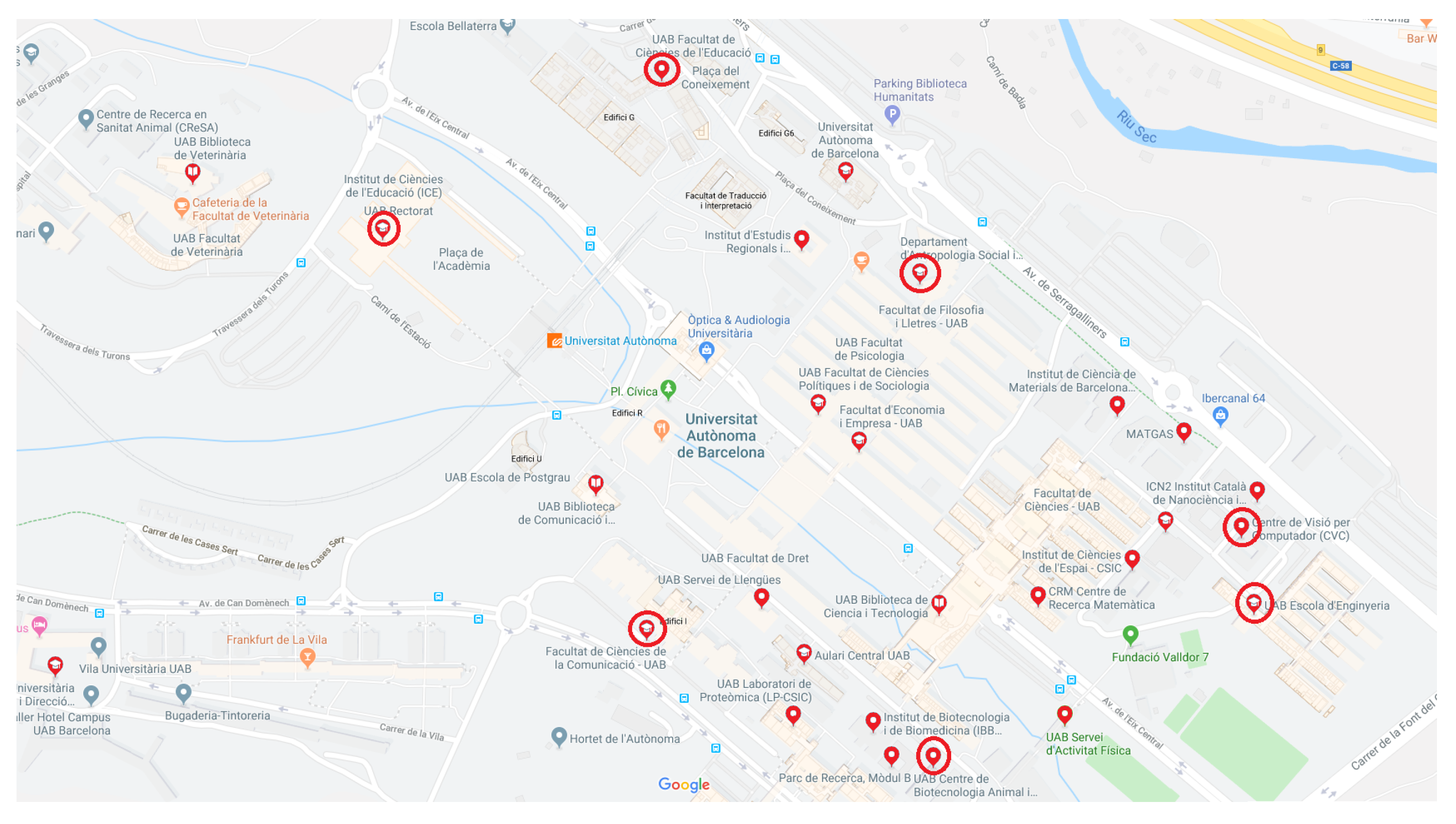
We first present to the students a statement of a salesperson type problem in a context based on a realistic situation that is located in a well-known environment, the university campus. The statement includes the following paragraph:
Every day, the postwoman of the university needs to go through all the faculties and other points that have mail. The points that have mail changes from one day to the other. Figure 9 shows an example: All possible points to deliver mail are marked in red check point, while points which has mail to deliver today are as well circled in red. The postwoman wants to deliver the mail to the target locations in the shortest possible time, and since she rides a bicycle we can consider that paths between locations are straight ones.
The problem statement also contains a caption of google maps with the target possible locations, like the one that is shown in
Figure 9.
The students are then asked to generate a way of problem representation that later will enable them to solve the problem using computational techniques. To this end, a discussion is promoted in the classroom, so that the mental models with which the students internally represent the situation are shared and it is possible to articulate a real model that aimed at mobilizing knowledge about the real world articulated with mathematical and computer knowledge.
The students conclude that the best abstract representation of the problem is by means of a graph, which they already well-know. They have been studied graphs from a theoretical point of view and have explored their coding in previous courses of the degree. During the session, students give meaning to each of the elements of the graph in order to adjust it to the needs of the problem. This process is guided by the teacher in order to have a common frame of reference that fits the features of GbPExplorer. They identify vertices, edges, and differences between locations and visits: to simplify, vertices are two-dimensional (2D) points in the plane and edges correspond to the Euclidean distance between two vertices.
Figure 10 shows the real model developed.
6.2. Moving to the Mathematical Model: GbPExplorer
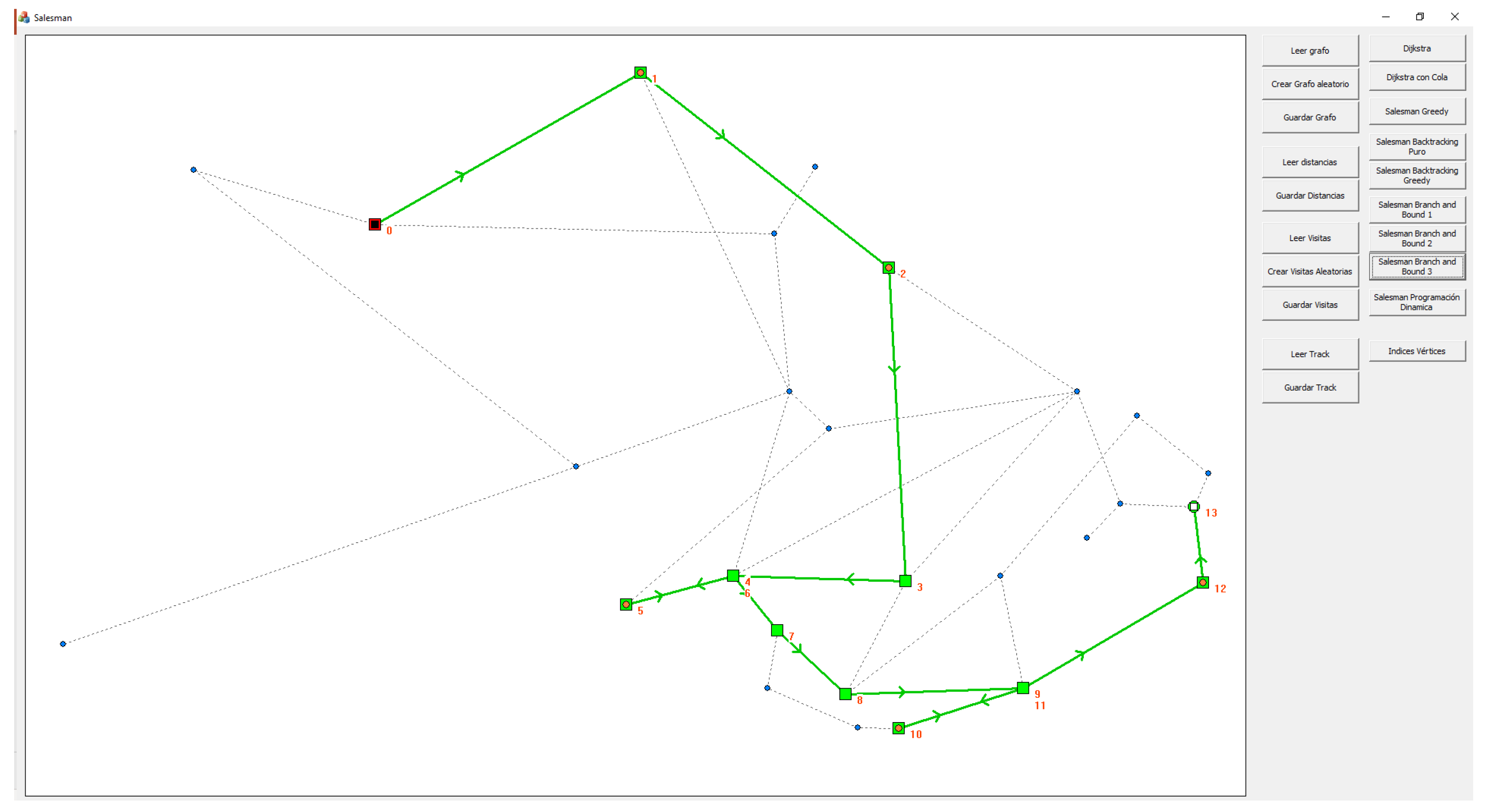
At this point, the teacher introduces the GbPExplorer to the students and explains its aim, the different modules that compose it and the way that it can help them during the project. In particular, the students can try to generate random situations and load the ones from the given dataset to check their optimal tracks. The first task to deliver is to design a particular graph and load it in the interface, in order to let students to familiarize with the use of GbPExplorer.
Figure 11 shows the visualization of the graph introduced on the map in
Figure 10 in the GbPExplorer, with the optimal solution marked as a directed subgraph in green.
Later, the teacher introduces the code behind the graphical interface in order to show data structures and explain the rest of the project. From here, the students will have to work on coding the different algorithmic techniques, as we explain them in the next sessions. An example of the code done by a student is shown in
Listing 3.
6.3. Creating Solutions and Comparing Methods
Returning to the adjusted cycle, as shown in
Figure 8, each coloured arrow means a different algorithmic technique to be coded. In this way, the students work on the implementation of different techniques for the same problem, which provides them with a background to compare them based on the obtained results. Later, they will work specifically on methods to make these comparisons in an objective way.
As we explained in
Section 5, once students code a particular technique, they can self-evaluate their performance by two different ways:
Visual graphical representation: once an algorithm is executed by the GbPExplorer, the solution track is printed in green. If the graph is small students can check if the algorithm builds the solution in the expected order. Additionally, if this solution contains any non existing vertex or edge, then it is marked in red and the student can rapidly realize.
Log information: for the graphs dataset, students obtain several text files with the track obtained by the algorithms together with the optimal solutions, the execution times, and the errors detected.
Here, are some examples of error checking.
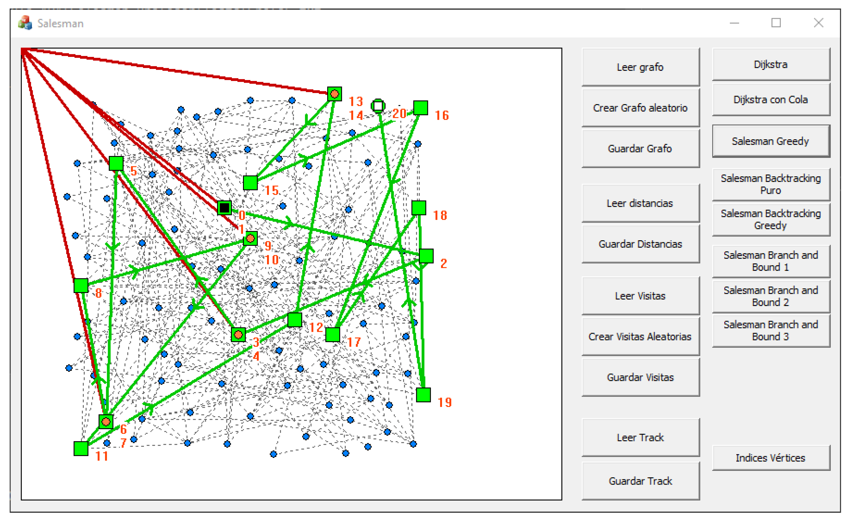
Figure 12 shows non-existing vertices, which are printed at point (0,0). Since these vertices connect to other ones by non existing edges, the last are printed in red.
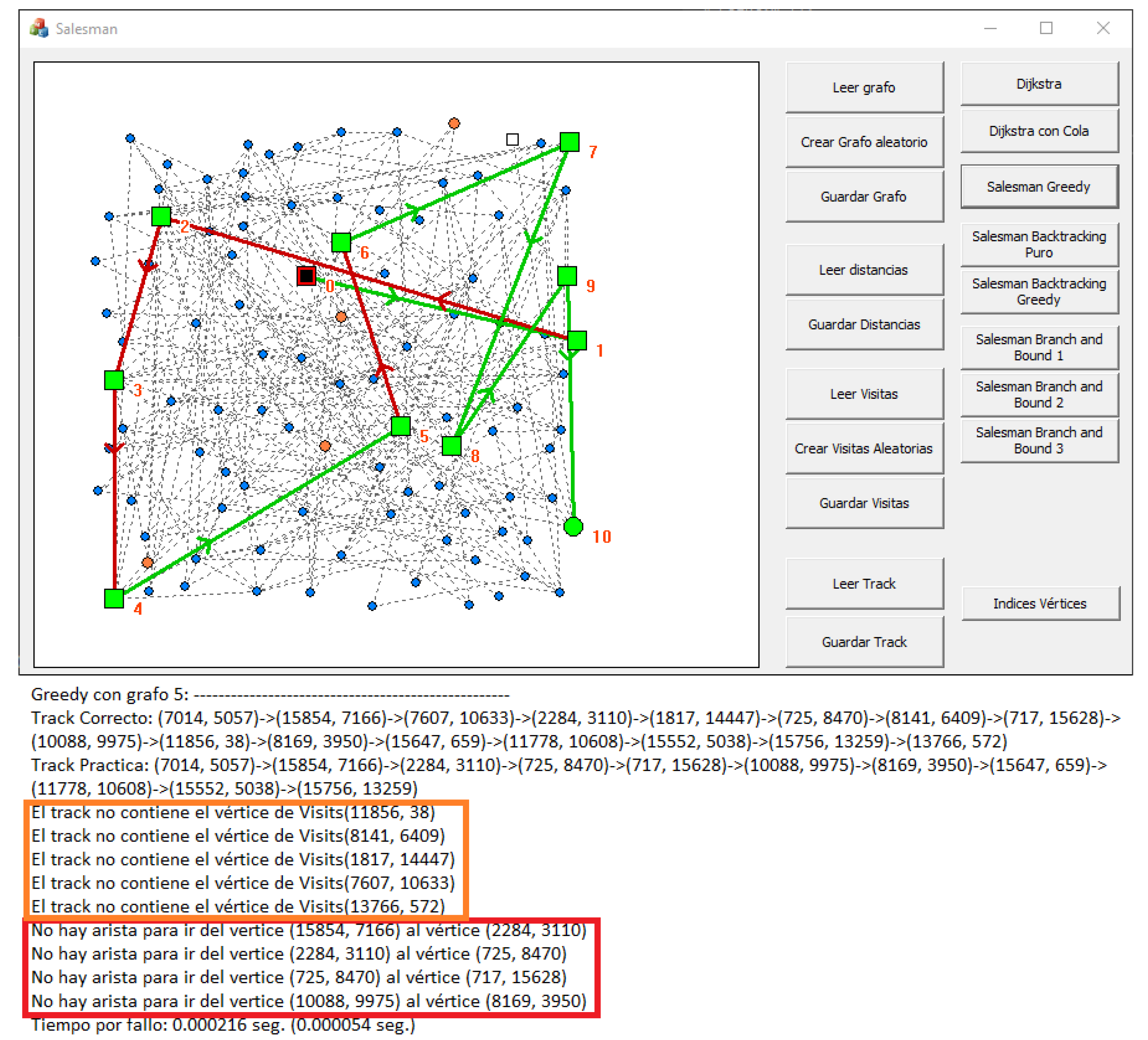
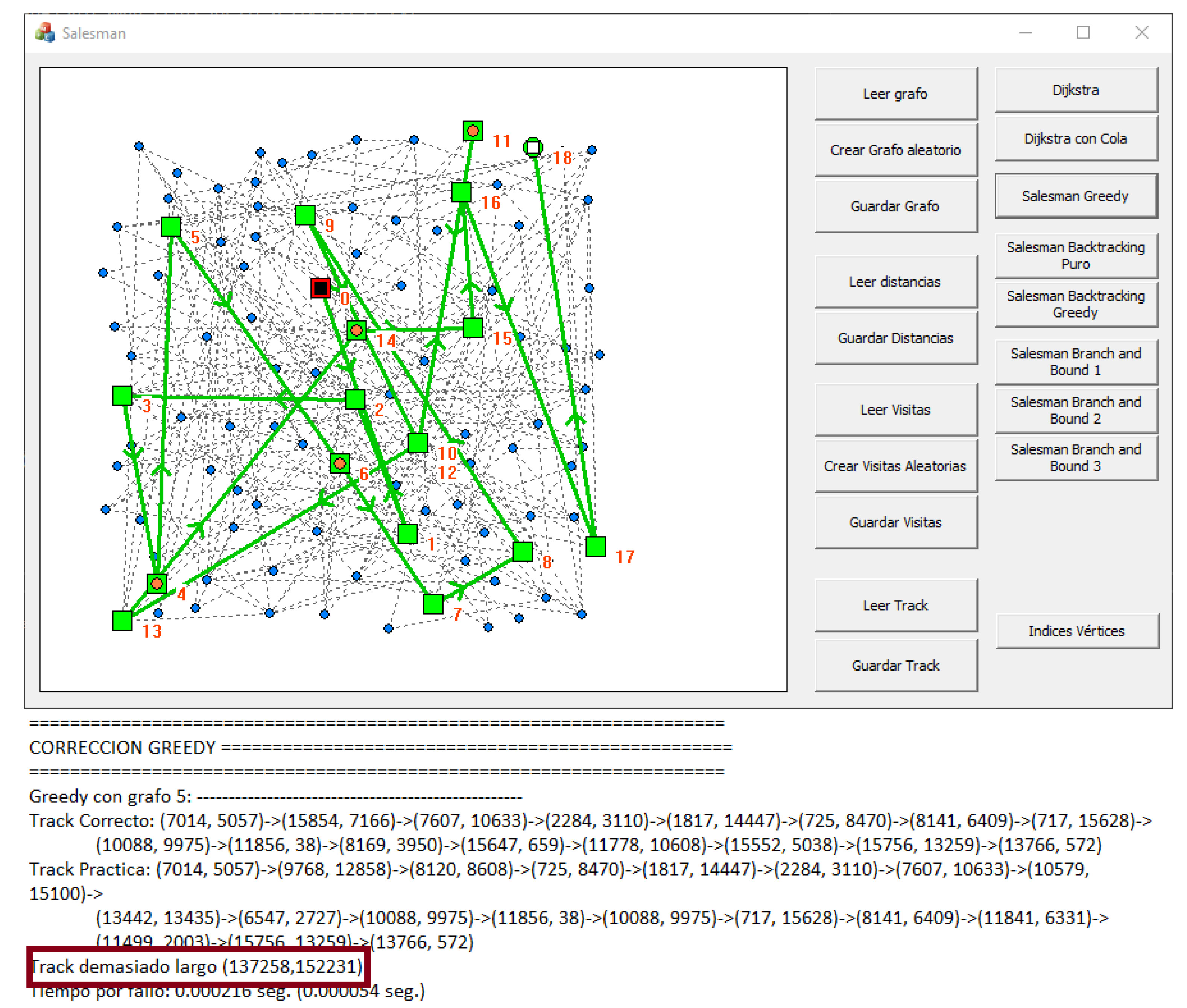
Figure 13 shows two different errors. On the one hand, the track obtained joins several vertices by non-existent edges, which can visually be observed in red. Additionally, the log points out these errors by a message, which can be observed in the bottom of the figure (boxed in red). On the other hand, there remain some unvisited vertices to visit, which can also be observed in orange, but, also, text log warns about it to reinforce the message (boxed in orange in the figure).
Figure 14 shows another type of error, which cannot be appreciated visually only. The track accomplishes all of the restrictions of the problem, but it is suboptimal. In the log, we can observe that the solution that is given by the student is longer than the optimal one as well as a warning message (boxed in red).
Finally, once the students have developed all the techniques, they have to analyse and compare them from the point of view of their computational complexity. This part of the project allows for them to connect the knowledge acquired during the project on the algorithmic techniques with the needs of real world and, at the same time, act as a validation process of their methods and results. Additionally, they need to have some clear concepts concerning to basic properties of graphs and computational complexity.
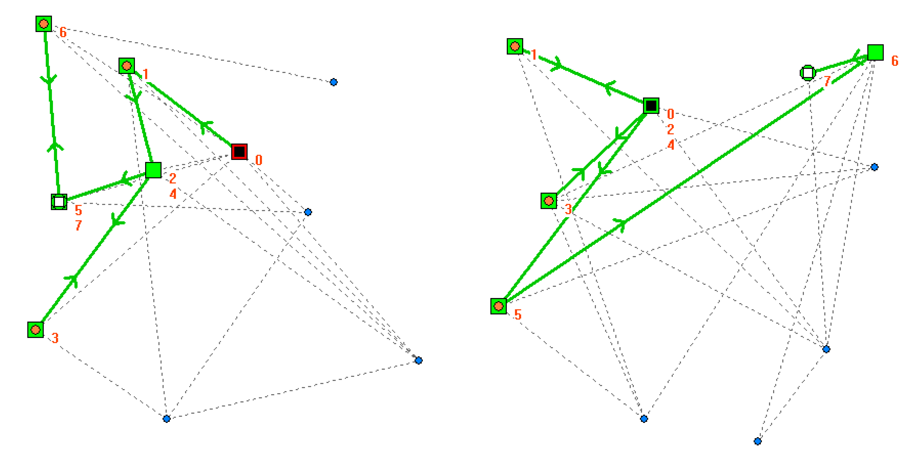
For the analysis, students have to pose different graphs, varying edges, vertices, and visits, and explore algorithms behaviour according to the execution time results. However, these times can be different in different executions on graphs with the same input parameters. For example,
Figure 15 shows an example of two different graphs with the same initial constrains (10 vertices, 20 edges, and five visits) with different runtimes and the GbPExplorer allows for them to realize it.
One class session is dedicated to discuss how to assess the computational performance of an algorithm and compare among several ones and, at the end, they deliver a report with their analysis results.
To study the performance of the algorithmic techniques, the students can use the GbPExplorer in two main ways: they can run the graphical interface as many times as they need and write down, in a spreadsheet, the execution times that the program outputs or they can modify the base code to obtain several solutions with different constrains (number of vertices, edges, and visits) at the same time.
Figure 16 shows two plots from a student’s report used for justifying his/her answer to the following question:
“How does the runtime of algorithms increases as the number of vertices increase? Which computational complexity have each algorithmic technique?”
On the left hand, we can observe a line for each algorithmic technique while on the right hand, there is one less. The student has observed that the grey line on the left might hinder the real visualization of the behaviour of the other plots, so that on the right hand (s)he has been suppressed.
In this way, teachers can focus on proposing different types of questions to students. For example, they can discuss what happens with execution times on backtracking algorithms when the initial constrains are changed, or which heuristic in branch and bound could be better, the ones that prioritize branching or the ones that prioritize optimizing data structures concerning vertices to visit.
7. Conclusions
Teaching computer science is a challenge for university teachers. The content of university programmes contains a large number of complex methods that have required great ideas and/or long development, and the students are expected to understand, master, and apply them in a short period of time. In recent years, attention has been redirected towards promoting the development of students’ skills, not only to learn content in a synthetic way, but to be able to use it effectively in real environments. To this end, in the case of analysis and design of algorithms, PBL appears as an educational framework in which to work with modelling. PBL requires that open, sometimes ill-defined, situations be offered to students to promote the development of skills, the interconnection of prior knowledge with new learning, and work in group. From the point of view of teachers, it is beneficial to have proposals for specific activities that include all of the complexity of the process to be worked on, while focusing on specific aspects at each step.
In this paper, we have presented a sequence of activities based on the theoretical framework of mathematical modelling that allows us to identify the key processes to be proposed to students. In this sense, we assume that university teachers know in detail the procedure to solve the problem. However, we claim that it is also necessary for them to base their teaching proposals on how their students will be able to understand each of the phases of the solution.
Additionally, we have shown the design of a software tool that supports the learning objectives of the sequence of activities. We claim that it is important that the tools that support computer-based learning contain various elements: (1) they must allow for a visualization that can refer to the real problem to be studied; (2) they must allow different types of exploration, from simple cases that could be solved on paper to the most complex ones; and, (3) they must integrate a set of automatic testers that provide detailed information to the students when they generate the codification of their methods. It is important to emphasize that those variables included in the application to evaluate methods will be the ones that students will end up valuing as useful.
GbPExplorer and the activities shown in this article can be easily adapted to work with other optimization problems that can be modelled using graphs. Even more, we would like to emphasize that the theoretical framework supporting the sequence of activities and the characteristics of the software tool can be adapted to a very wide range of work proposals in other STEM fields. In any STEM discipline, working in a guided way on the resolution of a complex problem, comparing techniques and methods for its resolution, is key to sustain competence in decision making. However, we understand that the transfer of the framework should be properly adapted to each content or discipline to ensure the achievement of didactic objectives, established in each case.
In the last five courses we have designed and refined the project activities and the layout of the GbPExplorer and we have been able to observe two didactic benefits. On the one hand, it has allowed us to focus on subject competences, rather than pure contents. This enables a methodological change, not only in the classroom, but also in the evaluation. As a consequence, students focus their efforts on developing their skills, beyond the expertise of a set of concrete techniques. In this fashion, students develop a more sophisticated level of self-awareness and explicitness about resolution strategies associated with mathematical modelling. On the other hand, this intervention also has an impact on the number of students making good progress, reducing the percentage of students who drop out of the course. With the use of GbPExplorer students now have specific tools that allow them to establish connections between theoretical content and the way in which they are used in the real world, as well as having support that is more in line with their learning needs. This aspect is relevant beyond the subjects presented in this paper as it allows the establishment of a way of engaging working for students and customizable to other subjects. Consequently, a working dynamic could be created to address the STEM curricula, helping to overcome some of the difficulties identified [
2].


