2.1. Identification of Pump Models
Head pressure–flow rate (H-Q) relationship is a mechanical characteristic of a pump which can be determined from the laboratory tests. It provides a convenient interface for incorporating the pump model to a model of the cardiovascular system as a nonlinear compartment. The two options for deriving the H-Q relationship are the usage of (semi-)empirical formulas and the derivation from the physical principles. In rather general form
is a quadratic form which is sometimes extended with the terms of the flow and pump rotation accelerations
. Here
H is the head pressure,
Q is the flow through the pump,
is the rotation speed of the pump rotor. The Euler head equation with added quadratic term
due to experimental evidence and the flow inertia term [
15] gives Model 1:
A similar model [
16] with the rotational acceleration of the pump defines Model 2:
The steady-flow model based on the conservation laws of mass, momentum and energy [
17] yields Model 3:
An addition to Model 3 of unsteady-flow effects and periphery parts [
14] results in Model 4:
where
is the pressure in the junction of the pump outlet and aorta,
is the pressure in the LV,
We note that Model 4 is not actually an H-Q relationship. It also includes parameters of the external (periphery) part which connects the pump to the LV and the aorta. The physical background of (
4) is discussed in [
14]. The theoretical Euler head equation gives the terms proportional to
and
. The fluid friction losses produce quadratic growth
with the flow elevation. The flow detachment at the leading and trailing edges of the blade produces eddy and separation losses proportional to
,
and
. Part-load recirculation in the blade channels occurs below the design flow rate. It partly blocks the channels, decreases their effective diameter and increases the head pressure introducing
term. The flow inertia term is proportional to
. Fluid friction and inertia frequency-dependent losses in the peripheral part are included via
in (
6). See [
14] and references herein for more details.
All the pump models (
1)–(
4) have physical interpretation. They were successfully validated with experimental data from different pumps in [
14,
15,
16,
17]. We take all these models as possible candidates for the H-Q mathematical relationship of non-pulsatile axial flow LVADs Sputnik D, Sputnik 1 and Sputnik 2. We use data from laboratory experiments with physical models of the paediatric mock circulation with Sputnik D [
8,
9,
10] and the adult mock circulation with Sputnik 1 and Sputnik 2 [
8,
12] for validation. Sensors are placed as close to the pumps as possible, thus, we exclude peripheral term
from (
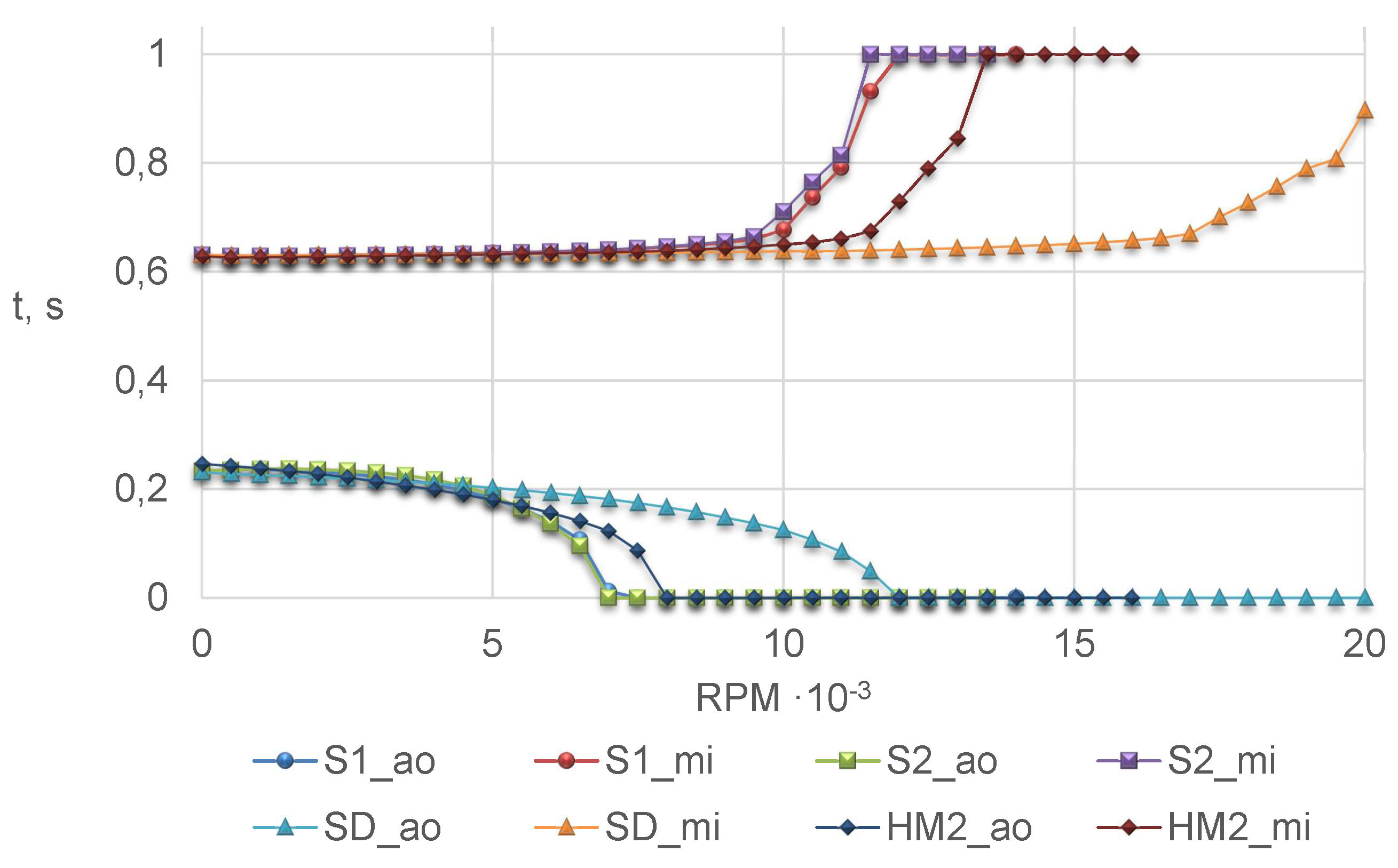
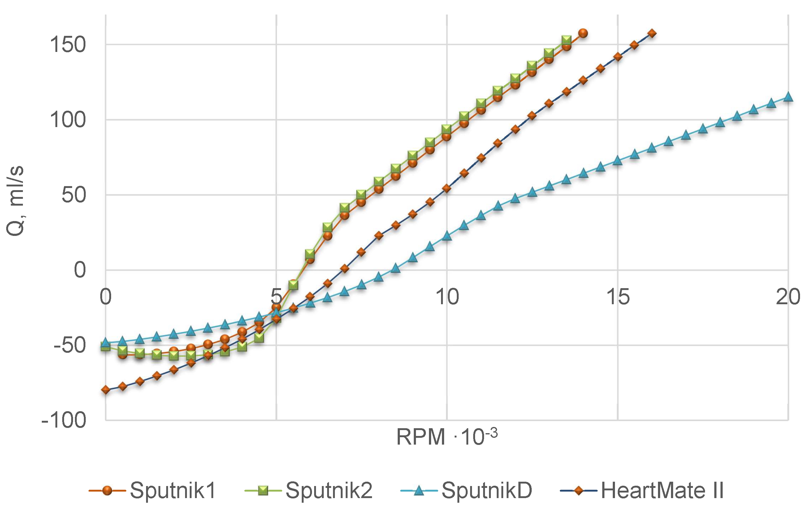
4) at the model fitting stage. Experimental setup imitates physiological conditions, including the Frank-Starling autoregulation mechanism of the heart which regulates the cardiac output depending on the ventricle preload. The 32% aqueous glycerol solution was used as the model fluid. Head pressure–flow rate (H-Q) curves for Sputnik D, Sputnik 1 and Sputnik 2 were measured at various constant pump speeds. For Sputnik D, the data from the range
–
rpm with the step
rpm were used as the training dataset, and the data from the range
–
rpm were used as the test dataset. For Sputnik 1 and Sputnik 2 the data from the range
–
rpm with the step 200 rpm and a contractility factor of the artificial LV 0.25 were used as the training dataset and the data from the range
–
rpm and the contractility factor of the artificial LV 0.5 were used as the test dataset. The contractility factor [
8] is a coefficient which decreases the end-systolic elasticity.
We set head pressure
H as a target variable. The parameters of the models were identified by the damped least-squares method (Levenberg–Marquardt algorithm) [
18,
19]. We smooth up the raw data by Savitzky–Golay filter [
20] for computing time derivatives of the flow and the rotational speed of the pump. The coefficient of determination
was used as the best-fit criterion. According to results presented in
Table 1, Model 4 provides the best fit with experimental data for all Sputnik pumps.
Table 2 comprises identified parameters of Sputnik pumps for Model 4, as well as Model 4 parameters of the LVAD HeartMate II from [
14]. Due to the lack of experimental data for Sputnik pumps periphery, we use mean values of the corresponding parameters for HeartMate II from [
14].
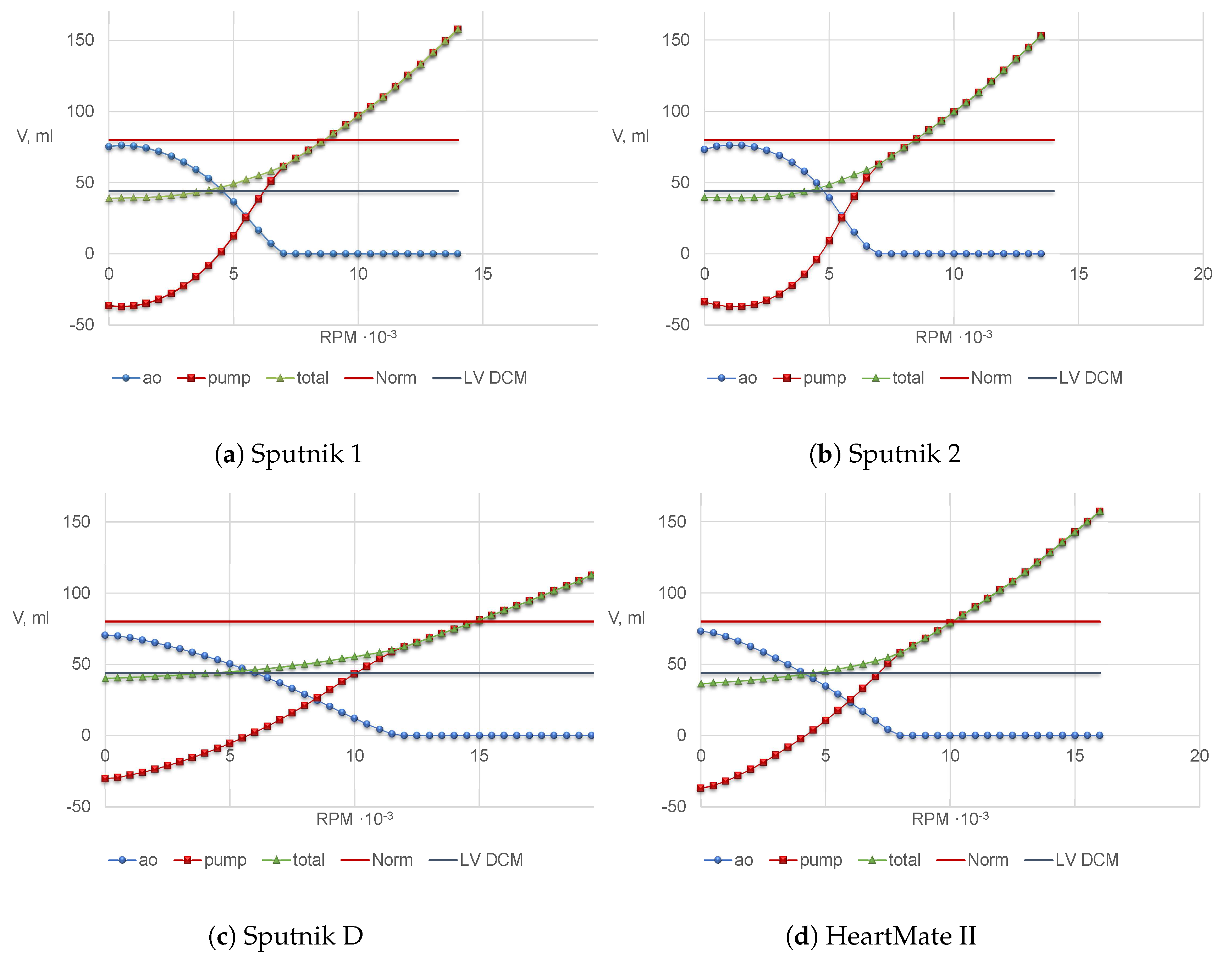
In the following sections, we incorporate Model 4 into a lumped model of the heart coupled with a 1D model of the aorta.
2.2. 1D Mathematical Model of the Blood Flow in Aorta Segments
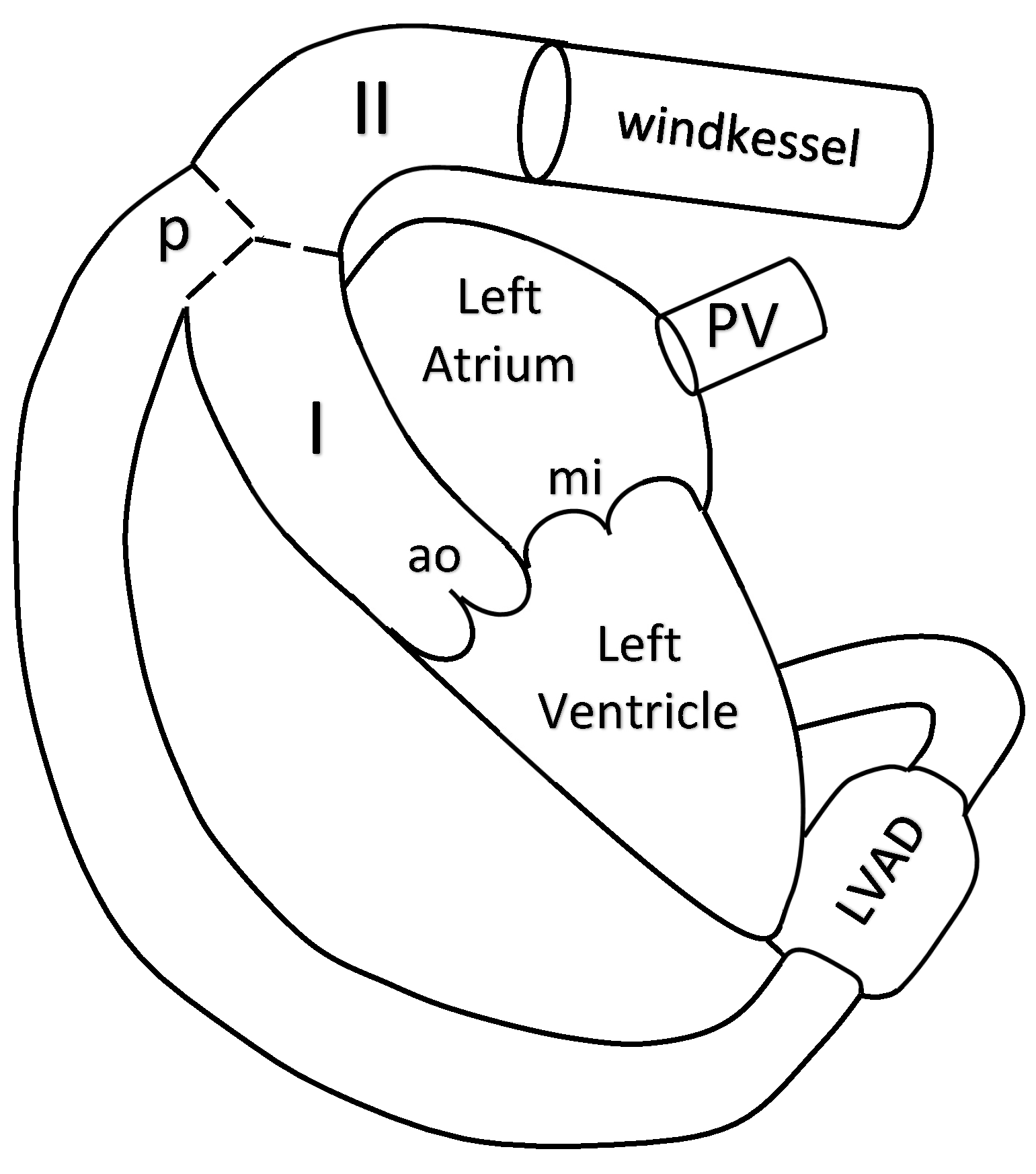
The blood flow in the aorta is simulated by a 1D reduced-order model of unsteady flow of viscous incompressible fluid in elastic tubes. The aorta is divided into two segments. The 1D model of the aorta is connected to the LV at the inlet, to the Windkessel compartment at the outlet and to the pump compartment between its segments I and II (see
Figure 1).
Reviews and details of 1D haemodynamic models can be found in [
21,
22,
23,
24,
25]. Algorithms of patient-specific parameter identification of such models were suggested in [
26,
27]. In this section, we briefly present this approach. We consider two 1D segments of the aorta which correspond to two parts of the ascending aorta (I and II in
Figure 1). We assume that the pump is connected to the aorta at the aortic arch before the carotid arteries. The flow in every vessel is described by mass and momentum conservation equations
where
t is the time,
x is the distance along the vessel counted from the vessel junction point,
is the blood density (constant),
is the vessel cross-section area,
p is the blood pressure,
is the linear velocity averaged over the cross-section,
is the friction force
is the dynamic viscosity of the blood. The elasticity of the vessel wall material is characterised by the
relationship
where
is the velocity of small disturbances propagation in the vessel wall,
is the monotone S-like function (see [
28] for the review of other options)
is the cross-sectional area of the unstressed vessel.
The mass conservation condition at the aortic root includes the blood flow through the aortic root
which is also a variable of the heart model from
Section 2.3:
Boundary conditions at the connection of aorta and the pump include mass conservation condition
and the continuity of the total pressure
where
is the static pressure at the output of the pump,
is the flow through the pump contributing to (
4),
is the cross-section area of the tube which connects the output of the pump and the aorta.
The outflow boundary conditions assume that the terminal part of the aorta is connected to the Windkessel compartment which describes the rest of the systemic circulation
where
are parameters presented in
Table 3,
is pressure in the Windkessel compartment.
The formulations of boundary conditions at the aortic root (
11), at the connection of the aorta and the pump (
12), (
13) and at the terminal part of the aorta (
14)–(
16) include a numerical discretisation of compatibility condition along the characteristic curve of the hyperbolic system (
7) which leaves the integration domain for every incoming and/or outgoing segment of the aorta (see [
21,
22,
23] for details). The systems of nonlinear algebraic equations, which represent boundary conditions with the time discretisation of the differential part are numerically solved by the Newton’s method.
The hyperbolic system (
7) inside every segment is numerically solved by the second order grid-characteristic method (see [
29] for the details of the method and [
21,
22] for the features of its implementation to the 1D model of the blood flow). The analysis of the characteristic curves of (
7) and similar formulations of 1D blood flow model allows implementing discontinuous Galerkin method [
30,
31]. The deep analysis of the quasilinear effects in a hyperbolic model blood flow through compliant axi-symmetric vessels can be found in [
32]. The generalised approach to the numerical implementation of the models describing various nonlinear wave process on graphs is described in [
33].
The parameters of the 1D model are given in
Table 3. The cross-sectional area and the length of the aortic segments I and II are set according to [
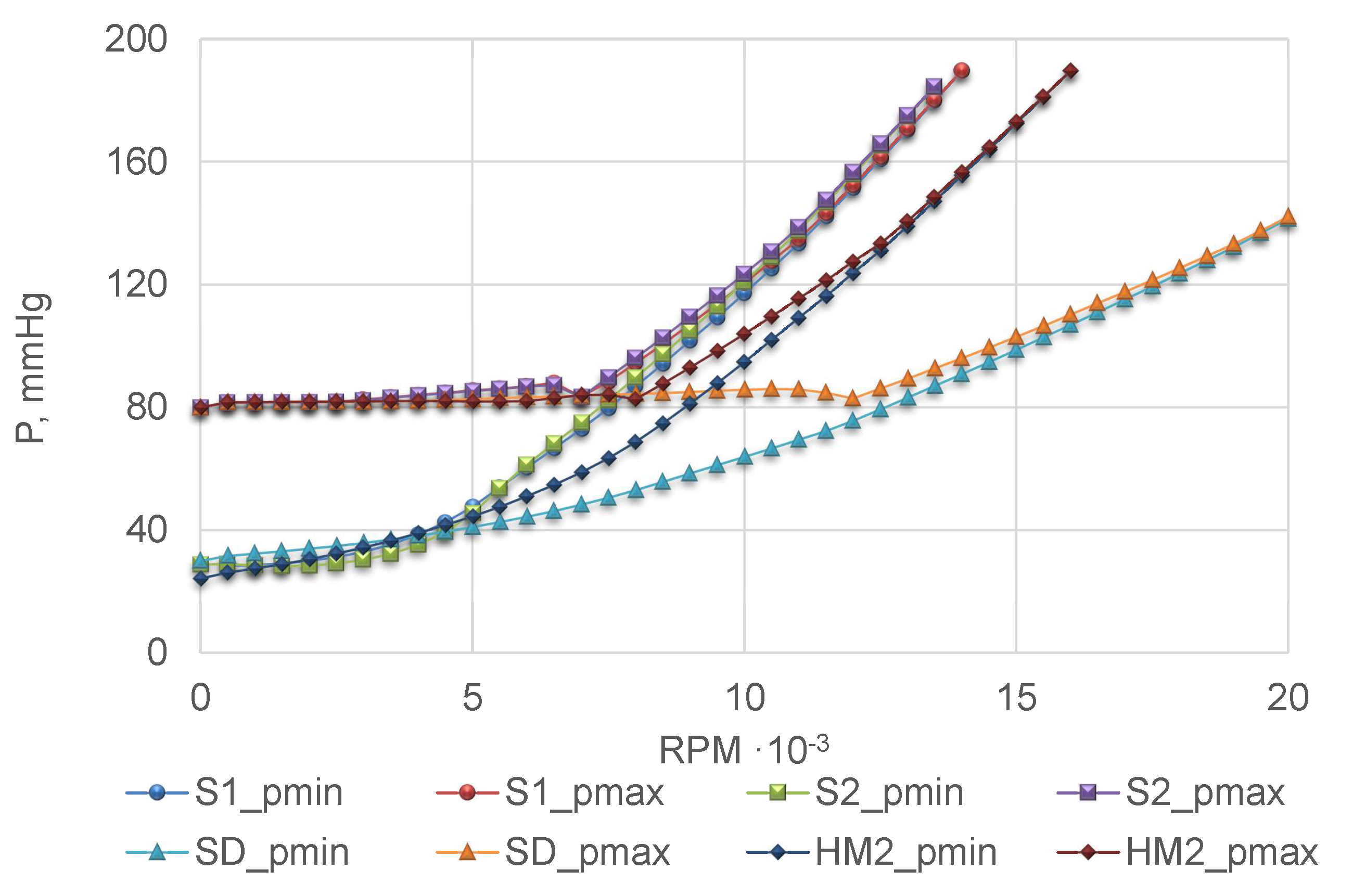
34]. The parameters of the Windkessel compartment are set manually. These values allow us to achieve the well known systolic and diastolic aortal pressures in the normal conditions (rf.
Section 3.1). For
and
we use the well known values [
35].
2.3. Integrated Mathematical Model of the Heart Function, Pump and Aortic Flow
The two chamber model of the heart comprises the LV and the left atrium (LA), the mitral and aortic valves. It connects the pulmonary veins (PV) with the aorta. The nonlinear LVAD compartment connects the LV with the aorta (see
Figure 1). The variable elasticity concept of the heart contractions [
36,
37] allows describing the heart chambers dynamics by the following lumped compartment model
where
, indices
and
refer to the LV and the LA, respectively,
is the volume of the chamber,
is the reference volume of the chamber,
is the pressure in the chamber,
is the reference pressure in the chamber,
is the inertia coefficient of the chamber,
is the hydraulic resistance coefficient of the chamber,
is variable elasticity which is approximated by
and
are elasticity constants related to the end diastolic and end systolic states of chamber
k (rf.
Table 4). For the LV we set
whereas for the LA
Here we modify the model [
38] by adding to (
17) the term proportional to
, which accounts for viscoelasticity of the myocardium [
39,
40,
41]. The values of constants
,
,
,
are presented in
Table 4.
The mass conservation law for the LV and LA states
where
is the flow through the mitral valve,
is the flow through the aortic valve,
is the flow through the pump,
is the flow from the PV.
We set the pressure drop
for PV – LA connection,
for LA – LV connection, and
for LV – AA connection. For unsteady flow in a channel with a variable cross-section, the pressure drop satisfies the relation [
39,
42]
where
is a smooth monotone function of the angle of a valve opening
[
43]:
The value
corresponds to the closed valve, while the value
corresponds to the opened valve. For
,
we have linear Poiseuille pressure drop condition which also accounts for the viscous friction losses. By analogy with [
44,
45] we neglect this term and set
for all cases. For
,
we have the orifice pressure drop condition. The first term in (
22) accounts for the inertia of non-stationary flow. The coefficient
is defined as [
42,
46,
47]
where parameters
,
and
are defined in
Table 4 whereas
. For the PV – LA connection
. For both mitral and aortic valves, their cross-section
depends on the angle of the valve opening,
.
The dynamics of the aortic and mitral valves is governed by the second Newton law. Pressure gradient across the valve, vorticity generation and shear forces acting on the valve leaflets [
48] have to be accounted in the model, rf. [
43,
49]. In this work we set valve dynamics equations as
where
is the angle of the aortic valve opening,
is the angle of the mitral valve opening,
,
,
,
are parameters presented in
Table 4, the first term at the right-hand side corresponds to the friction force, the second term corresponds to the pressure force driving the valve motion,
is the force which helps to avoid physiologically abnormal valve positions (
and
)
The other forces are neglected.
Parameters of the lumped model of the left heart are summarized in
Table 4. We take some values from [
38,
41,
43] and set other values manually basing on the values from [
38,
43] and keeping them in the physiological range.

 ,
, 


