Financial Distress Prediction and Feature Selection in Multiple Periods by Lassoing Unconstrained Distributed Lag Non-linear Models

Abstract

In this paper, we propose a new framework of a financial early warning system through combining the unconstrained distributed lag model (DLM) and widely used financial distress prediction models such as the logistic model and the support vector machine (SVM) for the purpose of improving the performance of an early warning system for listed companies in China. We introduce simultaneously the 3~5-period-lagged financial ratios and macroeconomic factors in the consecutive time windows t − 3, t − 4 and t − 5 to the prediction models; thus, the influence of the early continued changes within and outside the company on its financial condition is detected. Further, by introducing lasso penalty into the logistic-distributed lag and SVM-distributed lag frameworks, we implement feature selection and exclude the potentially redundant factors, considering that an original long list of accounting ratios is used in the financial distress prediction context. We conduct a series of comparison analyses to test the predicting performance of the models proposed by this study. The results show that our models outperform logistic, SVM, decision tree and neural network (NN) models in a single time window, which implies that the models incorporating indicator data in multiple time windows convey more information in terms of financial distress prediction when compared with the existing singe time window models.

1. Introduction

Over the last four decades, models and methods for the prediction of corporate financial distress have attracted considerable interest among academics as well as practitioners. Financial distress prediction models can be used for many purposes including: monitoring of the solvency of regulated companies, assessment of loan default risk and the pricing of bonds, credit derivatives, and other securities exposed to credit risk (see [1,2,3,4]).

Different countries have different accounting procedures and rules; thus, the definition of financial distress put forward by different scholars is not always the same (see [4,5,6,7]). Bankruptcy is one of the most commonly used outcomes of financial distress of a company [5]. The nature of a bankrupt firm is that the owners can abandon the firm and transfer ownership to the debt holders, and bankruptcy occurs whenever the realized cash flow is less than the debt obligations [8]. It is generally agreed on that financial failure leads to substantive weakening of profitability of the company over time, but it is also feasible that a financially distressed firm may not change its formal status to bankrupt [9]. Therefore, in this paper, as done by [3] and [4], we identify a financially distressed company as the one at risk of failing, but which remains a viable entity at the present time. More specifically, “special treatment” (ST) is used to measure the financial distress status of a listed company. Further, in this paper, we provide a group of financial distress prediction models that incorporate the panel data of financial and macroeconomic indicators to implement early financial distress prediction.

In the existing studies, many classical statistical methods, such as discriminant analysis [1]; logistic regression and multinomial logit models (see [2,3,4,10]); heuristic algorithm methods such as the genetic algorithm and particle swarm optimization [11]; currently popular machine learning techniques, such as the support vector machine, decision tree and neural networks (see [7,12,13,14,15,16]), have been widely applied to develop financial distress prediction models. The relevant studies also realize that a set of indicators can be used to predict the financial distress, including financial indicators (e.g., see [7,17,18,19,20]) and macroeconomic indicators (e.g., see [4]). For example, accounting models such as Altman’s 5-variable (Z-score) model (see [1]), 7-variable model (see [21]) etc. have gained popularity in both academic and industrial fields due to their discriminating ability and predictive power.

A few extant studies have predicted financial distress by using the accounting ratios from one or more years prior to its observation, given that early change in financial indicators may provide the warning sign of deterioration of financial conditions. The authors of [1] provide the evidence that bankruptcy can be predicted two years prior to the event, while those of [4] construct respectively two groups of financial distress prediction models for two periods: one year and two years before the observation of the financial distress event. They found that the models in the both time-windows have good predictive performance. Other similar examples can be found in [7,20,22].

In the relevant literatures, financial indicators in the different time windows have proven their contribution to the performance of the distress prediction models, in spite of the fact that the degree of their impact tends to change over time. However, the procedures are performed for all the different lag periods separately, i.e., only using information of one specific year prior to the date of the distress event. To the best of the authors’ knowledge, no previous study, which solves the listed companies’ financial distress prediction problem, takes into account the impacts of relevant indicators in the different and consecutive lag periods.

In this study, we take the form of the distributed lag model (DLM), in addition to classical classification techniques, into the financial distress prediction problem and propose a group of distress prediction models including the logistic-distributed lag model and the SVM-distributed lag model that can be treated as generalized distributed lag model. We construct the linkage between multiple lagged values of financial ratios and macroeconomic indicators and current financial status in order to capture the dynamic natures of the relevant data. Further, we propose to implement the penalized logistic-distributed lag financial distress model with the least absolute shrinkage and selection operator (lasso) penalty via the algorithm framework of the alternating direction method of multipliers (ADMM) that yields the global optimum for convex and the non-smooth optimization problem. Lasso-type penalty was applied for three purposes: to avoid the collinearity problem in applying the distributed lag models directly, to simultaneously select significant variables and estimate parameters, and to address the problem of over-fitting. We conduct a series of empirical studies to illustrate the application of our distributed lag financial distress models, including a comparison of predictive performances of the two distributed lag financial distress models proposed in this paper as well as the comparisons of predictive performances of our models with a group of widely used classification models in the different time windows. The results show that all distributed lag financial distress models aggregating the data in three consecutive time windows outperform the ones that incorporate the data in any single-period: 3 years, 4 years or 5 years before the observation year of financial distress, when the financial and macroeconomic factors are included. This paper may provide a means of improving the predictive performance of financial distress model by incorporating data of financial and macroeconomic indicators in consecutive and multiple periods before the observation of financial distress.

The rest of this paper is organized as follows. Section 2 briefly reviews the previous financial distress prediction literature and distributed lag modeling. Section 3 constructs a group of generalized distributed lag models composed of lagged explanatory variables and l₁ regularization, the logistic regression-distributed lag model and the lasso–SVM model with lags, and proposes the ADMM algorithm framework for coefficient estimations and variable selection at same time. Section 4 provides a description of the data. Section 5 presents the empirical results and compares the predictive performance of our models reflecting the extended lag effects of used indicators with the existing financial distress prediction models. Section 6 concludes the paper.

2. Background

2.1. Literature on Financial Distress Prediction

2.1.1. Financial Factors and Variable Selection

There is a large amount of theoretical and empirical microeconomic literature pointing to the importance of financial indicators on financial distress forecasting. The authors of [1] selected five financial indicators of strong predictive ability from the initial set of 22 financial indicators using stepwise discriminant analysis: earnings before interest and taxes/total assets, retained earnings/total assets, working capital/total assets, market value equity/book value of total debt and sales/total assets, which measures the productivity of assets of a firm. The other studies that concern the similar accounting ratios in financial distress prediction can also be found in [23,24]. Furthermore, the current-liabilities-to-current-assets ratio used to measure liquidity (see [22,25]) and the total-liabilities-to-total-assets ratio used to measure the degree of indebtedness of a firm (see [22,25,26]) and cash flow (see [18]) have been incorporated into the distress prediction models because of their predictive performance. The authors of [20] considered nine financial indicators and use them to predict the regulatory financial distress in Brazilian electricity distributors. The authors of [7] introduced 31 financial indicators and found that the most important financial indicators may be related to net profit, earnings before income tax, cash flow and net assets. Along this line, with machine learning methods developing, more diversified financial indicators have been considered in very recent studies of Hosaka [27], Korol et al. [28], and Gregova et al. [29].

Another very important recent research line in the area of financial distress prediction is the suitability problem of these financial ratios used as explanatory variables. For example, Kovacova et al. [30] discussed the dependence between explanatory variables and the Visegrad Group (V4) and found that enterprises of each country in V4 prefer different explanatory variables. Kliestik [31] chose eleven explanatory financial variables and proposed a bankruptcy prediction model based on local law in Slovakia and business aspects.

In this paper, we construct an original financial dataset including 43 financial ratios. The ratios are selected on the basis of their popularity in the previous literature (see [1,7,27]) and potential relevancy to this study. Then, like many relevant studies [32,33,34], we use the lasso method and conduct feature selection in order to exclude the potentially redundant factors.

2.1.2. Macroeconomic Conditions

Macroeconomic conditions are relevant for the business environment in which firms are operating; thus, the deterioration of macroeconomic conditions may induce the occurrence of the financial distress. Macroeconomic variables have been found to impact corporate default and bankruptcy risk significantly, and good examples can be found in [35,36,37,38,39]. In the aspect of financial distress of listed companies, [4] consider the macroeconomic indicators of the retail price index and the short-term bill rate adjusted for inflation in addition to the accounting variables. The results in their studies suggest that all macroeconomic indicators have significant impact on the likelihood of a firm’s financial distress. In this paper, we control for macroeconomic conditions, GDP growth, inflation, unemployment rate in the urban area and consumption level growth over the sample period. GDP growth is widely understood to be an important variable to measure economic strength and prosperity, and the increase in GDP growth may decrease the likelihood of distress. The authors of [22,40] have pointed out that the decline in GDP is significantly linked to the tightening of a firm’s financial conditions, especially during the financial crisis period. The unemployment rate and inflation are two broadly used measures of overall health of the economy. High unemployment and high inflation that reflect a weaker economy may increase the likelihood of financial distress. Their impacts on financial distress have been examined in [16,37].

Different from the existing relevant studies that consider the lagged effect of macroeconomic variables only in a fixed window, such as 3 years prior to financial distress [16], this paper imposes a distributed lag structure of macroeconomic data, in addition to financial ratio data, and considers the lagged effects of the factors in the multi-periods. Particular attention is devoted to the lag structure and whether the predicting performance can be improved after introducing a series of lagged macroeconomic variables. The theoretical and empirical investigations in this study may complement the literature on financial distress prediction concerned with applying dynamic macro and financial data.

2.1.3. Related Literature on Chinese Listed Companies

The Chinese stock market has grown to over 55 trillion in market capitalization as of February 2020, and the number of listed firms has surpassed 3200, becoming the world’s second largest market. Its ongoing development and the parallel evolution of regulations have made China’s stock market an important subject for mainstream research in financial economics [41]. In April 1998, the Shanghai and Shenzhen stock exchanges implemented a special treatment (ST) system for stock transactions of listed companies with abnormal financial conditions or other abnormal conditions. According to the regulations, there are three main reasons for designation of a ST company: (1) a listed company has negative net profits for two consecutive years; (2) the shareholders’ equity of the company is lower than the registered capital; (3) a firm’s operations have stopped and there is no hope of restoring operations in the next 3 months due to natural disasters, serious accidents, or lawsuits and arbitration [7]. ST status is then usually applied as a proxy of financial distress (e.g., [7,16,42,43,44,45]).

Researchers regard the topic of financial distress prediction of Chinese listed companies as data-mining tasks, and use data mining, machine learning or statistical methods to construct a series of prediction models incorporating financial data (see [7,42,43]) or financial plus macroeconomic data [16] in one-time-period, but not in multiple periods of time. In the very recent study of [45], the authors proposed a financial distress forecast model combined with multi-period forecast results. First, with the commonly used classifiers such as the support vector machine (SVM), decision tree (DT) etc., the two to five-year-ahead financial distress forecast models are established one by one and denoted as T-2 to T-5 models, respectively. Then, through combining the forecast results of these one-time-period models, the multi-period forecast results, as a weighted average over a fixed window, with exponentially declining weights, are provided. This is obviously different from our model, as we introduce the multi-period lagged explanatory variables and detect simultaneously the effects of the variables in different prior periods on financial distress in the process of modeling.

2.2. Distributed Lag Models

Sometimes the effect of an explanatory variable on a specific outcome, such as the changes in mortality risk, is not limited to the period when it is observed, but it is delayed in time [46,47]. This introduces the problem of modeling the relationship between a future outcome and a sequence of lags of explanatory variables, specifying the distribution of the effects at different times before the outcome. Among the various methods that have been proposed to deal with delayed effects, as a major econometric approach, distributed lag models (DLMs) have been used to diverse research fields including assessing the distributed lag effects of air pollutants on children’s health [48], hospital admission scheduling [49], and economical and financial time series analysis [50,51].

DLMs model the response Y_t, observed at time t in terms of past values of the independent variable X, and have a general representation given by

$$g\left(Y_t\right)={\alpha }_0+{{\displaystyle \sum }}_{l=0}^L{s}_l\left(x_{t-l};{\alpha }_l\right)+{\epsilon }_t,t=L,+1, \dots , T$$

(1a)

where Y_t is the response at time t and g is a monotonic link function; the functions s_l denote a smoothed relationship between the explanatory vector x_t−l and the parameter vector α_l; α₀ and ε_t denote the intercept term and error term with a zero mean and a constant variance σ²; l, L are the lag number and the maximum lag. The form that link function g takes presents a distributed lag linear model or a non-linear model. For example, linear g plus the continuous variable Y_t present distributed lag linear models, while the logit function g plus the binary variable Y_t present a distributed lag non-linear model. In model (1a), the parametric function s_l is applied to model the shape of the lag structure, usually polynomials (see [49,52]) or less often regression splines [53] or more complicated smoothing techniques of penalized splines within generalized additive models [47,48]. In fact, the introduction of s_l is originally used to solve the problem that these successive past observations may regard as collinear. If L, the number of relevant values of X, is small, as may well be the case for some problems if annual data are involved, then model (1a) degrades to an unconstrained distributed lag model given by the following general representation

$$g\left(Y_t\right)={\alpha }_0+{{\displaystyle \sum }}_{l=0}^L{\alpha }_l{}^T{x}_{t-l}+{\epsilon }_t, t=L,+1, \dots , T$$

(1b)

In (1b), the definitions of variables are the same as those in (1). Correspondingly, the coefficients in model (1b) can be estimated directly by pooled least squares for the linear case or pooled maximum likelihood for the non-linear case, e.g., logit link function g under the assumption that x_t−l is strictly exogenous [54].

In this paper, logistic regression with an unconstrained distributed lag structure is used to identify the relationship between financial and macroeconomic indicators and future outcome of financial distress. The logistic regression may be the most frequently used technique in the financial distress prediction field ([4,20]) because logistic regression relies on fewer assumptions due to the absence of the need for multivariate normality and homogeneity in the variance–covariance matrices of the explanatory variables [23]. Further, a lasso penalty is introduced to conduct simultaneous parameter estimation and variable selection, considering that the lasso penalty method has good performance for solving the overfitting problem caused by the introduction of factors in adjacent windows and selecting the features and the corresponding exposures with relatively significant influence on the response. In fact, the lasso method has been applied for linear-distributed lag modelling (e.g., [55]).

3. Methodology

In this section, by combining the logistic regression method and unconstrained distributed lag model, we seek to estimate which indicators and in which period prior to the distress event best predicts financial distress. First, we construct Model 1 that represents the “accounting-only” model and incorporates the financial ratios. We introduce the 3-period-lagged financial ratios as independent variables into Model 1 and use the model to predict the financial distress event in year t by using the data of relevant indicator of the consecutive years, t − 3, t − 4, t − 5, simultaneously. Note that t refers to the current year in this paper. Then, we construct Model 2, which represents the ‘accounting plus macroeconomic indicators’ model, and includes, in addition to the accounting variables, 3-period-lagged macroeconomic indicators. Then, we introduce lasso penalty to the models and implement the coefficient estimation and feature selection. Further, we provide the algorithm framework of alternating direction method of multipliers (ADMM) that yields the global optimum for convex and the non-smooth optimization problem to obtain the optimal estimation for the coefficients. Finally, we propose a support vector machine model that includes the lagged variables of the accounting ratios and macroeconomic factors. This model is used for comparison of the predictive performance of the logistic model with a distributed lag of variables.

3.1. Logistic Regression Framework with Distributed Lags

3.1.1. The Logistic Regression-Distributed Lag Model with Accounting Ratios Only

The logistic regression may be the most frequently used technique in the financial distress prediction field and has been widely recognized ([11,20]). We propose a logistic model composed of lagged explanatory variables. Similar to the distributed lag linear model, the model has the following general form:

$$P\left(Y_{i,t}=1|X_{i,t-l}\right)=(1+\exp (-({\alpha }_0+{{\displaystyle \sum }}_{l=0}^L{\alpha }_{t-l}^T{X}_{i,t-l})){)}^{-1}, t=t_0+L,t_0+L+1, \dots , t_0+L+d$$

(2)

In (2), Y_i,t is a binary variable, and if Y_i,t =1, then it means that firm I at time t is a financially distressed company, otherwise, firm i (i = 1, 2, …, n) is a financially healthy company, corresponding the case of Y_i,t = 0; α₀ is intercept, and α_t−l = (α_t−l,1, α_t−l,2, …, α_t−l,p)^T is the coefficient vector for the explanatory variable vector X_i,t−l at time t−l; X_i,t−l is the p-dimension accounting ratio vector for firm i at time t − l, l = 0, 1, 2, …, L; l, L are the lag number and the maximum lag; t₀ is the beginning of the observation period and d is the duration of observation. The idea in (2) is that the likelihood of occurrence of the financial distress at time t for a listed company may depend on X measured not only in the current time t, but also in the previous time windows t − 1 through t − L.

In Formula (2), we assume a five-year effect and set the maximum lag L = 5, given that (1) the effect of the explanatory variable on the response variable may decline to zero in the time series data scenario; (2) the considered length of lag is not more than 5 years in most of the previous studies of financial distress prediction (see [1,7,37]). Besides, we set directly the coefficient α_t−0, α_t−1, α_t−2 for the variables in the current year and the previous two year before ST to be 0 vectors, because (1) the financial statement in the current year (year t) is not available for financial distressed companies labeled as in financial distress in year t, since the financial statement is published at the end of the year, but special treatment probably occurs before the publication; (2) designation of an ST company depends on the financial and operating situations of the previous year before the label of ST. Put simply, it is not meaningful to forecast ST risk 0, 1 or 2 years ahead (see [7,45]). Therefore, the logistic model containing the 3~5-period-lagged financial indicators, defined as Model 1, is presented as follows:

P(Y_i,t = 1) = (1 + exp(−α₀ − α_t−3^TX_i,t−3 − α_t−4^TX_i,t−4 − α_t−5^TX_i,t−5)⁻¹

(3)

In Equation (3), Y_i,t is binary response and is defined the same in (2); X_i,t−3, X_i,t−4 and X_i,t−5 are the p-dimensional financial indicator vectors of firm i observed in year t − 3, t − 4 and t − 5; α₀, α_t−3, α_t−4, α_t−5 are intercept terms and the coefficient vectors for the explanatory vectors X_i,t−3, X_i,t−4 and X_i,t−5, respectively, and α_t−l (l = 3, 4, 5) stands for the average effect of increasing by one unit in X_i,t−l on the log of the odd of the financial distress event holding others constants. Of course, in Model 1, we consider the effect of changes in financial ratios on financial distress probability during three consecutive years (t − 3, t − 4, t − 5).

3.1.2. The Logistic Regression-Distributed Lag Model with Accounting Plus Macroeconomic Variables

We further add the macro-economic factors into Equation (3) to detect the influence of macroeconomic conditions, in addition to financial indicators. Model 2, including both accounting variables and macroeconomic variables, takes the following form:

P(Y_i,t = 1) = (1 + exp(−α₀−α_t−3^TX_i,t−3−α_t−4^TX_i,t−4−α_t−5^TX_i,t−5−η_t−3^TZ_i,t−3−η_t−4^TZ_i,t−4−η_t−5^TZ_i,t−5))⁻¹

(4)

In Equation (4), Z_t−l (l = 3, 4, 5) represents the m-dimensional macroeconomic factor vector of year t − l; η_t−l (l = 3, 4, 5) is the coefficient vector for Z_i,t−l; the others are defined as in Equation (3). Similarly, η_j,t−3 + η_j,t−4 + η_j,t−4 represent the cumulative effects on log odd of the distress event of the j-th (j = 1, 2, …, m) macroeconomic factor.

Models 1 and 2, marked as Equations (3) and (4), can reflect the continued influence of the financial statement and macroeconomic conditions for multi-periods on the response; however, a considerable amount of potentially helpful financial ratios, macroeconomic factors and their lags may bring redundant information, thus decreasing the models’ forecast performances. In the following section, we implement feature selection by introducing lasso penalty into the financial distress forecast logistic models. Further, we provide an ADMM algorithm framework to obtain the optimal estimation for the coefficients.

3.2. The Lasso–Logistic Regression-Distributed Lag Model

There is currently much discussion about the lasso method. Lasso, as an l₁-norm penalization approach, has been actively studied. In particular, lasso has been used on the distributed lag linear model, and lasso estimators for coefficients are obtained through minimizing the residual sum of squares and the l₁-norm of coefficients simultaneously (e.g., [55]). For the logistic model with lagged financial variables (3), we can extend to logistic–lasso as follows in Equation (5):

$$\left({\widehat{\alpha }}_0,\widehat{\alpha }\right)=\underset{{\alpha }_0,\alpha }{argmin}f\left({\alpha }_0,\alpha |X_{i,t-3},X_{i,t-4},X_{i,t-5},Y_{i,t}\right)+\lambda {\Vert \alpha \Vert }_1\hspace{0.17em}$$

(5)

where

$$f\left({\alpha }_0,\alpha |X_{it},Y_{i,t}\right)={\displaystyle \sum }_{t=t_0+5}^{t_0+d}{\displaystyle \sum }_{i=1}^n(-Y_{i,t}\left({\alpha }_0+{\alpha }^T{X}_{it}\right)+\ln (1+\exp \{{\alpha }_0+{\alpha }^T{X}_{it}\}))$$

and ${\widehat{\alpha }}_0$ and $\widehat{\alpha }$ denote the maximum likelihood estimations for intercept α₀ and coefficient vector α; f denotes the minus log-likelihood function of Model 1 and can be regarded as the loss function of the observations; α = (α_t−3^T, α_t−4^T, α_t−5^T)^T are the unknown coefficients for explanatory variables; X_it = (X_i,t−3^T, X_i,t−4^T, X_i,t−5^T)^T, Y_i,t are known training observations and defined as above; λ is the turning parameter; ${\Vert ·\Vert }_1$ denotes l₁-norm of a vector, i.e., the addition of absolute values of each element of a vector; t₀ and d are defined as before; n is the number of observed company samples.

Introducing the auxiliary variable β ∈ R^3p, the lasso–logistic model (5) can be explicitly rewritten as follows:

$$\underset{{\alpha }_0,\alpha ,\hspace{0.17em}\beta }{min}f\left({\alpha }_0,\alpha |X_{i,t-3},X_{i,t-4},X_{i,t-5},Y_{i,t}\right)+\lambda {\Vert \beta \Vert }_1\hspace{0.17em}\hspace{0.17em}s.t.\alpha =\beta$$

(6)

In this paper, we solve the optimization problem (6) by using alternating direction method of multipliers (ADMM) algorithm that was first introduced by [56]. ADMM is a simple but powerful algorithm and can be viewed as an attempt to blend the benefits of dual decomposition [57] and augmented Lagrangian methods for constrained optimization [58]. Now, the ADMM algorithm becomes a benchmark first-order solver, especially for convex and non-smooth minimization models with separable objective functions (see [59,60]), thus, it is applicable for the problem (6).

The augmented Lagrangian function of the optimization problem (6) can be defined as

$$L_{\rho }\left({\alpha }_0,\alpha ,\beta ,\theta \right)=f({\alpha }_0,\alpha |X_{it},Y_{i,t})+\lambda {\Vert \beta \Vert }_1-{\theta }^T\left(\alpha -\beta \right)+\frac{\rho }{2}{\Vert \alpha -\beta \Vert }_2^2$$

(7)

where L_ρ is the Lagrange function; θ is a Lagrange multiplier vector and ρ(>0) is an augmented Lagrange multiplier variable. In this paper, ρ is predetermined to be 1 for simplicity. Then, the iterative scheme of ADMM for the optimization problem (6) reads as

$$\left({\alpha }_0^{k+1},{\alpha }^{k+1}\right)=\underset{{\alpha }_0,\alpha }{argmin}{L}_{\rho }\left(\left({\alpha }_0,\alpha \right),{\beta }^k,{\theta }^k\right)$$

(8a)

$${\beta }^{k+1}=\underset{\beta }{argmin}{L}_{\rho }\left({\alpha }^{k+1},\beta ,{\theta }^k\right)$$

(8b)

$${\theta }^{k+1}={\theta }^k-\rho \left({\alpha }^{k+1}-{\beta }^{k+1}\right)$$

(8c)

In (8a)–(8c), α₀^k+1, α^k+1, β^k+1, and θ^k are the values of α₀, α, β, and θ the k-th iterative step of the ADMM algorithm, respectively. Further, the ADMM scheme (8a)–(8c) can be specified as

$$\left({\alpha }_0^{k+1},{\alpha }^{k+1}\right)=\underset{{\alpha }_0,\alpha }{argmin}f\left({\alpha }_0,\alpha \right)-{({\theta }^k)}^T\left(\alpha -{\beta }^k\right)+\frac{\rho }{2}{\Vert \alpha -{\beta }^k\Vert }_2^2$$

(9a)

$${\beta }^{k+1}=\underset{\beta }{argmin}\lambda {\Vert \beta \Vert }_1-{({\theta }^k)}^T\left({\alpha }^{k+1}-\beta \right)+\frac{\rho }{2}{\Vert {\alpha }^{k+1}-\beta \Vert }_2^2$$

(9b)

$${\theta }^{k+1}={\theta }^k-\rho \left({\alpha }^{k+1}-{\beta }^{k+1}\right)$$

(9c)

The sub-problem in (9a), that is, the convex and smooth optimization problem, can be fast solved by the Newton method [61], after setting the initial θ, β to be arbitrary constants. More specifically, let α_*^k+1 = (α₀^k+1; α^k+1) and α_*^k+1 be calculated via the following process:

$${\alpha }_{*}^{k+1}={\alpha }_{*}^k-{({\nabla }^{2}l)}^{-1}\nabla l$$

(10)

where

$$l\left({\alpha }_{*}\right)=l\left({\alpha }_0;\alpha \right)=f\left({\alpha }_0,\alpha \right)-{({\theta }^k)}^T\left(\alpha -{\beta }^k\right)+\frac{\rho }{2}{\Vert \alpha -{\beta }^k\Vert }_2^2$$

and ${\nabla }^{2}l\in R^{\left(3p+1\right)\times \left(3p+1\right)}$, $\nabla l\in R^{3p+1}$ are the hessian matrix and the derivative of differentiable function l with respect to α_*, respectively. For sub-problem (9b), its solution is analytically given by

$${\beta }_r^{k+1}=\{\begin{array}{c}{\alpha }_r^{k+1}-\frac{\lambda +{\theta }_r^k}{\rho },{\alpha }_r^{k+1}>\frac{\lambda +{\theta }_r^k}{\rho }\hfill \\ 0,\frac{-\lambda +{\theta }_r^k}{\rho }<{\alpha }_r^{k+1}\le \frac{\lambda +{\theta }_r^k}{\rho }\hfill \\ —, {\alpha }_r^{k+1}\le \frac{-\lambda +{\theta }_r^k}{\rho }\hfill \end{array}$$

(11)

where β_r^k+1, α_r^k+1 and θ_r^k are the r-th components of β^k+1, α_r^k+1 and θ^k, respectively, for the k-th iterative step and r = 1, 2, …, 3p.

The choice of tuning parameters is important. In this study, we find an optimal tuning parameter λ by the 10-fold cross validation method. We then compare the forecast accuracy of each method based on the mean area under the curve (MAUC) given as follows:

$$MAUC\left(\lambda \right)={\displaystyle \sum }_{j=1}^{10}AU{C}^j\left(\lambda \right)/10$$

(12)

where AUC^j(λ) denotes the area under the receiver operating characteristic (ROC) curve on j-th validation set for each tuning parameter λ.

So far, the lasso estimators for the logistic model (5) including 3~5-period-lagged financial ratios have been obtained by following the above procedures. For the convenience of readers, we summarize the whole optimization procedures in training the lasso–logistic with lagged variables and describe them in Algorithm 1.

Algorithm 1. An alternating direction method of multipliers (ADMM) algorithm framework for lasso–logistic with lagged variables (5). 1: Dual residual and prime residua denote ||βk+1 − βk||2 and ||αk+1 − βk+1||2 respectively. 2: N denotes the maximum iterative number of the ADMM algorithm.

Require: Training data {Xi,t−3, Xi,t−4, Xi,t−5, Yi,t }, where Xi,t−l∈RP, l = 3, 4, 5 and Yi,t∈{0,1}, i = 1, 2, …, n, t = t0 + 5, t0 + 6, …, t0 + d Turning parameter λ Choose augmented Lagrange multiplier ρ = 1. Set initial (θ0, β0) ∈ R × RP, (α00,α0) ∈ R × RP and stopping criterion ε = 10−6. Ensure: 4. While not converging (i.e., dual residual and prime residual 1 are greater than stopping criterion of 10−6) do 5. Fork = 0, 1, …, N2 do 6. Calculate αk+1 following the Newton algorithm (10) 7. Calculate βk+1 following (11) 8. Update θk+1 ← θk − ρ(αk+1 − βk+1) 9.  End for 10. End while.

For the logistic model (4) with lag variables of the financial ratio and macroeconomic indicators, we can also extend the lasso as follows in (13):

$$\left({\widehat{\alpha }}_0,\widehat{\gamma }\right)=\underset{{\alpha }_0,\gamma }{argmin}f\left({\alpha }_0,\gamma |X_{i,t-3},X_{i,t-4},X_{i,t-5},Z_{i,t-3},Z_{i,t-4},Z_{i,t-5},Y_{i,t}\right)+\lambda {\Vert \gamma \Vert }_1$$

(13)

where $\widehat{\gamma }=\left(\widehat{\alpha },\widehat{\eta }\right)$ is the lasso estimator vector for coefficients of lagged financial ratios and macroeconomic indicators; γ = (α^T, η^T)^T represents the unknown coefficients for explanatory variables; α, η = (η_t−3^T, η_t−4^T, η_t−5^T)^T and the others are defined as in Equations (4) and (5). The lasso estimator for model (13) can also be found by using the ADMM algorithm presented above.

3.3. The Lasso–SVM Model with Lags for Comparison

The support vector machine (SVM) is a widely used linear classifier with high interpretability. In this sub-section, we construct a lasso–SVM model that includes the 3-period-lagged financial indicators for comparison with the lasso–logistic-distributed lag model. The SVM formulation combing the original soft-margin SVM model [62] and a 3~5--period-lagged financial ratio variable vector is as follows:

$$\{\begin{array}{c}\underset{{\alpha }_0,\alpha ,\xi }{min}\hspace{0.17em}\hspace{0.17em}\frac{1}{2}{\Vert \alpha \Vert }_2^2+C{\displaystyle {\displaystyle \sum }_{t=t_0+5}^{t_0+d}}{\displaystyle {\displaystyle \sum }_{i=1}^n}{\xi }_{i,t}\hfill \\ s.t.\hspace{0.17em}{Y}_{i,t}\left({\alpha }_0+{\alpha }_{t-3}{}^T{X}_{i,t-3}+{\alpha }_{t-4}{}^T{X}_{i,t-4}+{\alpha }_{t-5}{}^T{X}_{i,t-5}\right)\ge 1-{\xi }_{i,t},\hspace{0.17em}{\xi }_{i,t}\ge 0,\hfill \\ i=1,2,\dots ,n,\hspace{0.17em}t=t_0+5,\dots ,Id\end{array}$$

(14)

In (14), α₀ (intercept) and α = (α_t−3; α_t−4; α_t−5) (normal vector) are the unknown coefficients of hyper-plane f(X_it) = α₀ + α^TX_it; ${\Vert ·\Vert }_2$ denotes l₂-norm of a vector; C is the penalty parameter and a predetermined positive value; ξ_i,t is the unknown slack variable; Y_i,t is a binary variable and Y_i,t = 1, when firm i is a financially disIressed company in year t, otherwise Y_i,t = −1; X_it = (1; X_i,t−3; X_i,t−4; X_i,t−5) denotes the observation vector of 3~5-period-lagged financial indicators for firm i; n represents the number of observations; t₀ and d denote the beginning and length of the observation period, respectively.

By introducing the hinge loss function, the optimization problem (14) has the equivalent form as follows [63]:

$$\underset{{\alpha }_{*}}{min}{\displaystyle \sum }_{t=t_0+5}^{t_0+d}{\displaystyle \sum }_{i=1}^n{[1-Y_{i,t}\left({\alpha }_{*}{}^T{X}_{it}\right)]}_{+}+\lambda {\Vert {\alpha }_{*}\Vert }_2^2$$

(15)

where α_* = (α₀; α), [·]₊ indicates the positive part, i.e., [x]₊ = max{x,0}, and the turning parameter λ = 1/2C.

Considering that it is regularized by l₂-norm, the SVM forces all nonzero coefficient estimates, which leads to the problem of its inability to select significant features. Thus, to prevent the influence of noise features, we replace l₂-norm in the optimization problem (15) with l₁-norm, which is able to simultaneously conduct feature selection and classification. Furthermore, for computational convenience, we replace the hinge loss function in (15) with the form of the sum of square, and present the optimization problem combining the SVM model and the lasso method (l₁ regularization) as follows:

$$\underset{{\alpha }_{*}}{{\widehat{\alpha }}_{*}=argmin}{\displaystyle \sum }_{t=t_0+5}^{t_0+d}{\displaystyle \sum }_{i=1}^n{({[1-Y_{i,t}{\alpha }_{*}{}^T{X}_{it}]}_{+})}^2+\lambda {\Vert {\alpha }_{*}\Vert }_1$$

(16)

In (16), ${\widehat{\alpha }}_{*}$ is the optimal estimated value for the coefficients of the SVM model, and the others are defined as above. Similarly with the process of the solution to the problem (5) as presented previously, first by introducing an auxiliary variable β ∈ R^3p+1, the lasso–SVM model (16) can be explicitly rewritten as follows:

$$\underset{{\alpha }_{*},\beta }{min}{\displaystyle \sum }_{t=t_0+5}^{t_0+d}{\displaystyle \sum }_{i=1}^n{({[1-Y_{i,t}{\alpha }_{*}{}^T{X}_{it}]}_{+})}^2+\lambda {\Vert {\beta }_{*}\Vert }_1\hspace{0.17em}\hspace{0.17em}\hspace{0.17em}s.t.\hspace{0.17em}{\alpha }_{*}={\beta }_{*}$$

(17)

Then, the augmented Lagrangian function of the optimization problem (17) can be accordingly specified as

$$L_{\rho }\left({\alpha }_{*},{\beta }_{*},{\theta }_{*}\right)={\displaystyle \sum }_{t=t_0+5}^{t_0+d}{\displaystyle \sum }_{i=1}^n{({[1-Y_{i,t}{\alpha }_{*}{}^T{X}_{it}]}_{+})}^2+\lambda {\Vert {\beta }_{*}\Vert }_1-{\theta }_{*}{}^T\left({\alpha }_{*}-{\beta }_{*}\right)+\frac{\rho }{2}{\Vert {\alpha }_{*}-{\beta }_{*}\Vert }_2^2$$

(18)

where θ ∈ R^3p+1 and ρ ∈ R are the Lagrange and the augmented Lagrange multipliers, respectively. Then, the iterative scheme of ADMM for the optimization problem (18) is similar with (8a)–(8c) and can be accordingly specified as

$${\alpha }_{*}{}^{k+1}=\underset{{\alpha }_{*}}{argmin}{\displaystyle \sum }_{t=t_0+5}^{t_0+d}{\displaystyle \sum }_{i=1}^n{({[1-Y_{i,t}\left({\alpha }_{*}{}^T{X}_{it}\right)]}_{+})}^2-{({\theta }_{*}{}^k)}^T\left({\alpha }_{*}-{\beta }_{*}{}^k\right)+\frac{\rho }{2}{\Vert {\alpha }_{*}-{{\beta }_{*}}^k\Vert }_2^2$$

(19a)

$${\beta }_{*}{}^{k+1}=\underset{{\beta }_{*}}{argmin}\lambda {\Vert {\beta }_{*}\Vert }_1-{\theta }^k\left({\alpha }_{*}{}^{k+1}-{\beta }_{*}\right)+\frac{\rho }{2}{\Vert {\alpha }_{*}{}^{k+1}-{\beta }_{*}\Vert }_2^2$$

(19b)

$${\theta }_{*}{}^{k+1}={\theta }_{*}{}^k-\rho \left({\alpha }_{*}{}^{k+1}-{\beta }_{*}{}^{k+1}\right)$$

(19c)

The finite Armijo–Newton algorithm [61] is applied for solving the α-sub-problem (19a), which is a convex piecewise quadratic optimization problem. Its objective function is first-order differentiable but not twice-differentiable with respect to α_*, which precludes the use of a regular Newton method. F(α_*) is the objective function of the sub-optimization problem (19a) and its gradient and generalized Hessian matrix are presented as follows Equations (20) and (21):

$$\nabla F\left({\alpha }_{*}\right)=-2{\displaystyle \sum }_{t=t_0+5}^{t_0+d}{\displaystyle \sum }_{i=1}^n{Y}_{i,t}{X}_{it}{(1-Y_{i,t}{\alpha }_{*}{}^T{X}_{it})}_{+}-{\theta }^k+\rho \left({\alpha }_{*}-{\beta }_{*}{}^k\right)$$

(20)

$${\partial }^{2}F\left({\alpha }_{*}\right)=2{\displaystyle \sum }_{t=t_0+5}^{t_0+d}{\displaystyle \sum }_{i=1}^{n}diag{(1-Y_{i,t}{\alpha }_{*}{}^T{X}_{it})}_{*}{X}_{it}{X}_{it}^T+\rho I$$

(21)

where I ∈ R^3p+1 is identity matrix and diag(1 − Y_i,t α_*^TX_it)_* is a diagonal matrix in that the j-th (j = 1, 2, …, 3p + 1) diagonal entry is a sub-gradient of the step function (·)₊ as

$${(diag{(1-Y_{i,t}{\alpha }_{*}{}^T{X}_{it})}_{*})}_{jj}\{\begin{array}{cc}=1\hfill & if\hspace{0.17em}\hspace{0.17em}1-Y_{i,t}{\alpha }_{*}{}^T{X}_{it}>0,\hfill \\ \in \left[0,1\right]\hfill & if\hspace{0.17em}\hspace{0.17em}1-Y_{i,t}{\alpha }_{*}^T{X}_{it}=0,\hfill \\ =0\hfill & if\hspace{0.17em}\hspace{0.17em}1-Y_{i,t}{\alpha }_{*}^T{X}_{it}<0.\hfill \end{array}$$

(22)

The whole optimization procedure applied to solve the α-sub-problem (19a) is described in Algorithm 2.

Algorithm 2. A finite Armijo–Newton algorithm for the sub-problem (19a). 1: δ is the parameter associated with finite Armijo Newton algorithm and between 0 and 1.

Require: Training data {Xi,t−3, Xi,t−4, Xi,t−5, Yi,t}, where Xi,t−l ∈ RP, l = 3, 4, 5 and Yi,t∈{1,−1}, I = 1,2,…, n, t = t0 + 5, t0 + 6,…, t0 + d Turining parameter λ Choose augmented Lagrange multiplier ρ = 1. Set initial (θ*0, β*0, α*0) ∈ R × R3P+1 × R3P+1 and stopping criterion ε = 10−6 Ensure: 4.  While not converging (i.e., ||▽F[(α*i) − ∂2F(α*i)−1▽F(α*i)]||2 ≥ ε) do 5. Calculate the Newton direction di = −∂2F(α*i)−1▽F(α*i) following (20)–(22) 6. Choose δ1 = 0.4 and find stepsize τi = max{1, 1/2, 1/4, …} such that F(α*i) − F(α*i + τi di) ≥ −δτi▽F(α*i)Tdi is satisfied 7. Update (α*)i+1 ← (α*)i + τi di, i ← I + 1 8.  End while 9. Output α*k+1 = α*i

The finite Armijo–Newton algorithm can guarantee the unique global minimum solution in a finite number of iterations. The details of proof of the global convergence of the sequence to the unique solution can be found in [61]. For the sub-problem (19b), its solution can be also analytically given by (11) presented above, after replacing α, β and θ with α_*, β_* and θ_*.

So far, the lasso estimators for the SVM model (16), including 3~5-period-lagged financial ratios, have been obtained by following the above procedures. For the convenience of readers, we summarize the whole optimization procedures in training the lasso–SVM with lagged variables and describe them in Algorithm 3. It is worth to note that the estimators for the lasso–SVM model that contain 3~5-period-lagged financial ratios and macro-economic indicators can be also obtained by the following algorithm similarly.

Algorithm 3. An ADMM algorithm framework for lasso–support vector machine (SVM) with lagged variables (16)

Require: Training data {Xi,t−3, Xi,t−4, Xi,t−5, Yi,t}, where Xi,t−l∈RP, l = 3, 4, 5 and Yi,t∈{1,−1}, i = 1, 2, …, n, t = t0 + 5, t0 + 6, …, t0 + d Turining parameter λ Choose augmented Lagrange multiplier ρ = 1. Set initial (θ*0, β*0, α*0)∈R × R3P+1 × R3P+1 and stopping criterion ε = 10−6 Ensure: 4. While not converging (i.e., either ||βk+1 − βk||2 or ||αk+1 − βk+1||2 is greater than stopping criterion of 10−6) do 5. Fork = 0, 1, …, N do 6. Calculate α*k+1 following finte Armijo–Newton algorithm displayed in Algorithm 2 7. Calculate β*k+1 following (11) 8. Update θ*k+1 ← θ*k − ρ(α*k+1 − β*k+1) 9.  End for 10.  End while

4. Data

4.1. Sample Description

The data used in the study are limited to manufacturing corporations. The manufacturing sector plays an important role in contributing to the economic growth of a country, especially a developing country [64]. According to the data released by the State Statistical Bureau of China, manufacturing accounts for 30% of the country’s GDP. China’s manufacturing sector has the largest number of listed companies as well as the largest number of ST companies each year. On the other hand, according to the data disclosed by the China Banking Regulatory Commission, in the Chinese manufacturing sector, the non-performing loan ratio has been increasing. For example, there was a jump in the non-performing loan ratio from 3.81% in December of 2017 to 6.5% in June of 2018. Therefore, it is quite important to establish an effective early warning system aiming to assess financial stress and prevent potential financial fraud of a listed manufacturing company for market participants, including investors, creditors and regulators.

In this paper, we selected 234 listed manufacturing companies from the Wind database. Among these, 117 companies are financially healthy and 117 are financially distressed, i.e., the companies being labeled as “special treatment”. The samples were selected from 2007 to 2017, since the Ministry of Finance of the People’s Republic of China issued the new ‘‘Accounting Standards for Business Enterprises’’ (new guidelines), which required that all listed companies be fully implemented from January 1, 2007. Similar to [7], [16] and [45], all 117 financially distressed companies receive ST due to negative net profit for two consecutive years. There were respectively 10, 9, 17, 24, 26 and 31 companies labeled as ST or *ST in each year from 2012 to 2017. The same number of financially healthy companies were selected in each year. Considering the regulatory requirement and qualified data of listed companies, our data sample enforces the use of 2007 (t₀) as the earliest estimation window available in forecasting a listed company’s financial distress. Meanwhile, the maximum order lag used in our models is as long as 5 (years); that is, the maximum horizon is 5 years, so the number of special-treated (ST) companies was counted since 2012 (t₀ + 5). Furthermore, we divided the whole sample group into two groups: the training sample and the testing sample. The training sample is from 2012 to 2016, includes the data of 172 companies and is used to construct the models and estimate the coefficients. Correspondingly, the testing sample is from 2017, includes the data of 62 companies and is used to evaluate the predicting performance of the models.

4.2. Covariate

In this paper, we use the factors measured in consecutive time windows t − 3, t − 4 and t − 5 to predict a listed company’s financial status at time t (t = 2012, 2013, …, 2017). Therefore, we define response y as whether a Chinese manufacturing listed company was labeled as “special treatment” by China Securities Regulatory Commission at time t (t = 2012, 2013, …, 2017) and input explanatory variables as their corresponding financial indicators based on financial statements reported at t − 3, t − 4 and t − 5. For example, we define response y as whether a Chinese manufacturing listed company was labeled as “special treatment” during the period of from January 1, 2017 to December 31, 2017 (denoted as year t) and (1) input explanatory variables as their corresponding financial indicators based on financial statements reported on December 31, 2014 (denoted as year t − 3), in December, 2013 (denoted as year t − 4) and in December, 2012 (denoted as year t − 5); through this way, the time lags of the considered financial indicators and the responses are between 3 to 5 years; (2) input explanatory variables as macroeconomic indicators based on the statements reported on December 31, 2014, 2013 and 2012 by the Chinese National Bureau of Statistics; through this way, the time lags of the considered macroeconomic indicators and the response are also between 3 to 5 years. The effect of time lags of 3 to 5 years of financial indicators on the likelihood of occurrence of financial distress is separately suggested by some previous research of early warnings of listed companies’ financial distress, but the varying effects of these time lags that occur in one prediction model are not yet considered in the existing studies.

4.2.1. Firm-Idiosyncratic Financial Indicator

An original list of 43 potentially helpful ratios is compiled for prediction and provided in

Table 1. List of financial indicators.

Solvency	Operational Capabilities
1 Total liabilities/total assets (TL/TA)	9 Sales revenue/average net account receivable (SR/ANAR)
2 Current assets/current liabilities (CA/CL)	10 Sales revenue/average current assets (SR/ACA)
3 (Current assets–inventory)/current liabilities (CA-I)/CL	11 Sales revenue/average total assets (AR/ATA)
4 Net cash flow from operating activities/current liabilities (CF/CL)	12 Sales cost/average payable accounts (SC/APA)
5 Current liabilities/total assets (CL/TA)	13 Sales cost/sales revenue (SC/SR)
6 Current liabilities/shareholders’ equity (CL/SE)	14 Impairment losses/sales profit (IL/SP)
7 Net cash flow from operating and investing activities/total liabilities (NCL/TL)	15 Sales cost/average net inventory (SC/ANI)
8 Total liabilities/total shareholders’ equity (TSE/TL)	16 Sales revenue/average fixed assets (SR/AFA)
Profitability	Structural Soundness
17 Net profit/average total assets (NP/ATA)	27 Net asset/total asset (NA/TA)
18 Shareholder equity/net profit (SE/NP)	28 Fixed assets/total assets (FA/TA)
19 (Sales revenue–sales cost)/sales revenue (SR-SC)/SR	29 Shareholders’ equity/fixed assets (SE/FA)
20 Earnings before interest and tax/average total assets (EIA/ATA)	30 Current liabilities/total liabilities (CL/TL)
21 Net profit/sales revenue (NP/SR)	31 Current assets/total assets (CA/TA)
22 Net profit/average fixed assets (NP/AFA)	32 Long-term liabilities/total liabilities (LL/TL)
23 Net profit attributable to shareholders of parent company/sales revenue (NPTPC/SR)	33 Main business profit/net income from main business (MBP/NIMB)
24 Net cash flow from operating activities/sales revenue (NCFO/SR)	34 Total profit/sales revenue (TP/SR)
25 Net profit/total profit (NP/TP)	35 Net profit attributable to shareholders of the parent company/net profit (NPTPC/NP)
26 Net cash flow from operating activities/total assets at the end of the period (NCFO/TAEP)	36 Operating capital/total assets (OC/TA)
	37 Retained earnings/total assets (RE/TA)
Business Development and Capital Expansion Capacity
38 Main sales revenue of this year/main sales revenue of last year (MSR(t)/MSR(t-1))	41 Net assets/number of ordinary shares at the end of year (NA/NOS)
39 Total assets of this year/total assets of last year (TA(t)/TA(t-1))	42 Net cash flow from operating activities/number of ordinary shares at the end of year (NCFO/NOS)
40 Net profit of this year/net profit of last year (NP(t)/NP(t-1))	43 Net increase in cash and cash equivalents at the end of year/number of ordinary shares at the end of year (NICCE/NOS)

because of the large number of financial ratios found to be significant indicators of corporate problems in past studies. These indicators are classified into five categories, including solvency, operational capability, profitability, structural soundness and business development and capital expansion capacity. All variables used for calculation of financial ratios are obtained from the balance sheet, income statements or cash flow statements of the listing companies. These financial data for financially distressed companies are collected in year 3, 4 and 5 before the companies receive the ST label. For example, the considered year when the selected financially distressed companies receive ST is 2017; the financial data are obtained in 2014, 2013 and 2012. Similarly, the data for financially healthy companies are also collected in 2014, 2013 and 2012. Model 1 (the accounting-only model) will be constructed using all the data in the following context. The model is used to predict whether a company is labeled in year t, incorporating the financial data of three consecutive time windows, t − 3, t − 4 and t − 5 (t = 2012, 2014, …, 2017).

4.2.2. Macroeconomic Indicator

Besides considering three consecutive period-lagged financial ratios for the prediction of financial distress of Chinese listed manufacturing companies, we also investigated the associations between macro-economic conditions and the possibility of falling into financial distress of these companies. The macro-economic factors include GDP growth, inflation, unemployment rate in urban areas and consumption level growth, as described in

Table 2. List of macroeconomic factors.

Figure 1	Description
1 Real GDP growth (%)	Growth in the Chinese real gross domestic product (GDP) compared to the corresponding period of previous year (GDP growth is documented yearly and by province).
2 Inflation rate (%)	Percentage changes in urban consumer price compared to the corresponding period of the previous year (inflation rate is documented regionally).
3 Unemployment rate (%)	The data derived from the Labor Force Survey (population between 16 years old and retirement age, unemployment rate is documented yearly and regionally).
4 Consumption level growth (%)	Growth in the Chinese consumption level index compared to the corresponding period of the previous year (consumption level growth is documented yearly and regionally).

¹: All data of the macro-economic covariates are collected from the National Bureau of Statistics of China.

. GDP growth is widely understood to be an important variable to measure economic strength and prosperity; the increase in GDP growth may decrease the likelihood of distress. High inflation and high unemployment that reflect a weaker economy may increase the likelihood of financial distress. Consumption level growth reflects the change in consumption level and its increase may reduce the likelihood of financial distress.

In the following empirical part, Model 2 represents the ”accounting plus macroeconomic indicators” model and includes, in addition to the accounting variables, 3-period-lagged macroeconomic indicators. We collected the corresponding macroeconomic data in each year from 2007 to 2012 for all 234 company samples and the raw macroeconomic data are from the database of the Chinese National Bureau of Statistics.

4.3. Data Processing

The results in the existing studies suggest that the predicting models of standardized data yield better results in general [65]. Therefore, before the construction of the models, a standardization processing is implemented based on the following linear transformations:

$$x_{ij}\left(t\right)=\frac{u_{ij}\left(t\right)-\underset{1\le i\le 234}{min}\left\{u_{ij}\left(t\right)\right\}}{\underset{1\le i\le 234}{max}\left\{u_{ij}\left(t\right)\right\}-\underset{1\le i\le 234}{min}\left\{u_{ij}\left(t\right)\right\}}\hspace{0.17em}$$

(23)

where x_ij(t) denotes the standardized value of the j-th financial indicator for the i-th firm in year t, and j = 1, 2, …, 43, i = 1, 2, …, 234, and t = 2007, 2008, …, 2012; u_ij(t) denotes the original value of the j-th indicator of the i-th company in year t. Linear transformation scales each variable into the interval [0, 1]. Similarly, the following formula is used for data standardization of the macro-economic factor:

$$z_{ij}\left(t\right)=\frac{v_{ij}\left(t\right)-\underset{1\le i\le 234}{min}\left\{v_{ij}\left(t\right)\right\}}{\underset{1\le i\le 234}{max}\left\{v_{ij}\left(t\right)\right\}-\underset{1\le i\le 234}{min}\left\{v_{ij}\left(t\right)\right\}}\hspace{0.17em}$$

(24)

In formula (24), z_ij(t) denotes the standardized value of the j-th macro-economic factor in year t; v_ij(t) denotes the original value of the j-th indicator of the i-th company in year t, where j = 1, 2, 3, 4, i = 1, 2, …, 234, and t = 2007, 2008, …, 2012. It is worth noting that the assignment to v_ij(t) for each company is based on the data of the macroeconomic condition of the province where the company operates (registration location).

5. Empirical Results and Discussion

In this chapter, we establish a financial earning prediction system for Chinese listed manufacturing companies by using two groups of lasso-generalized distributed lag models, i.e., a logistic model and an SVM model including 3~5-period-lagged explanatory variables, and implement financial distress prediction and feature selection simultaneously. For the selected sample set, the sample data from 2007 to 2016 were used as the training sample and the sample from 2017 as the test sample. The tuning parameter was identified from cross-validation in the training set, and the performance of the chosen method was evaluated on the testing set by the area under the receiver operating characteristics curve (AUC), G-mean and Kolmogorov–Smirnov (KS) statistics.

5.1. Preparatory Work

It is necessary to choose a suitable value for the tuning parameter λ that controls the trade-off of the bias and variance. As mentioned before, 10-fold cross-validation is used on the training dataset in order to obtain the optimal tuning parameter, λ. First, we compare prediction performance of the lasso–logistic-distributed lag model (5) including only 43 firm-level financial indicators (the accounting-only model) when the turning parameter λ changes. The results show that the mean AUCs of validation data are 0.9075, 0.9095, 0.9091, 0.9112, 0.8979, 0.8902 and 0.8779, respectively, corresponding to λ = 0.01, 0.1, 0.5, 1, 2, 3, 4. Second, we compare the prediction performance of the logistic-distributed lag model (4) incorporating lasso penalty with 43 firm-level financial indicators and 4 macro-economic factors (the model of accounting plus macroeconomic variables). The results show that the mean AUCs of validation data are 0.9074, 0.8018, 0.9466, 0.9502, 0.9466, 0.9466 and 0.8498, respectively, corresponding to λ = 0.01, 0.1, 0.5, 1, 2, 3, 4. Panel (a) and (b) in Figure 1 also show the average predictive accuracy of cross-validation that results from using seven different values of the tuning parameter λ in the accounting model and the model of accounting plus macroeconomic variables.

Generally speaking, the two kinds of models yield the best performance when λ = 1. Therefore, in the following, we fit and evaluate the lasso–logistic-distributed lag models by using the tuning parameter of 1.

5.2. Analyses of Results

This study develops a group of ex-ante models for estimating financial distress likelihood in the time window of t to test the contribution of financial ratios and macroeconomic indicators in the consecutive time windows of t − 3, t − 4 and t − 5. In the followings,

Table 3. The indicator selection and the estimates for lasso–logistic-distributed lag models.

Selected Indicator	Model 1 (Financial Ratios Only)			Model 2 (Financial Plus Macroeconomic Factor)
	t − 3	t − 4	t − 5 1	t − 3	t − 4	t − 5
1 Total liabilities/total assets	× 2	×	3.1671 (0.07) ***,3	×	×	3.5519 (0.07) ***
2 Current liabilities/total assets	×	−3.356 (0.27) ***	×	×	−1.2292 (0.26) ***	×
3 Sales revenue/average current assets	×	−0.5988 (0.19).	×	×	−3.887 (0.19) ***	×
4 Sales revenue/average total assets	−0.4367 (0.14) ***	−5.7393 (0.24) ***	−1.8312 (0.14) **	−0.5428 (0.14) **	−0.3907 (0.23) **	−3.5193 (0.14) ***
5 Sales cost/sales revenue	5.1892 (0.08) **	×	×	3.9211 (17.57)	×	×
6 Impairment losses/sales profit	−0.4496 (0.08) ***	×	×	−0.5777 (0.08) ***	×	×
7 Sales cost/average net inventory	−1.3265 (0.12) ***	×	×	−1.1143 (0.12) *	×	×
8 Net profit/average total assets	×	−1.1919 (0.14)	×	×	−3.3509 (0.14) **	×
9 Shareholders’ equity/net profit	5.4466 (0.17) ***	×	×	4.0804 (0.18) ***	×	×
10 (Sales revenue-sales cost)/sales revenue (net income/revenue)	×	×	×	−1.2209 (17.7)	×	×
11 Net profit/average fixed assets	1.3912 (0.31) **	×	×	×	×	×
12 Net profit/total profit	×	0.2856 (0.14) ***	0.0422 (0.09) *	×	0.0371 (0.14) ***	×
13 Net cash flow from operating activities/total assets	−4.8561 (0.11) ***	−2.6798 (0.11)**	−1.0999 (0.12)	−3.005 (0.1) *	−2.7581 (0.1) **	−0.0304 (0.12)
14 Fixed assets/total assets	1.6395 (0.1)	0.9142 (0.11) **	×	1.5972 (0.09)	×	0.5416 (0.09)
15 Shareholders’ equity/fixed assets	×	1.0914 (0.09) ***	×	×	0.0472 (0.09) **	×
16 Current liabilities/total liabilities	2.2516 (0.06) *	×	2.2987 (0.07) ***	3.1472 (0.06) ***	×	2.1535 (0.07) ***
17 Current assets/total assets	−1.5197 (0.11)	×	×	−3.081 (0.11) *	×	×
18 Long−term liabilities/total liabilities	×	1.6 (0.07) *	×	×	1.8855 (0.06) **	×
19 Main business profit/net income from main business	−3.3814 (0.1) ***	−1.0212 (0.1) ***	5.2777 (0.1) ***	−4.0263 (0.1) ***	−0.9392 (0.1) ***	5.876 (0.1) ***
20 Net profit attributable to shareholders of the parent company/net profit	−3.5409 (0.13) ***	×	×	−2.159 (0.13) ***	×	×
21 Operating capital/total assets	−2.1682 (0.16) ***	×	×	−0.328 (0.16) *	×	×
22 Main sales revenue of this year/main sales revenue of last year	×	×	2.9534 (0.1) **	×	×	2.5545 (0.11) **
23 Net assets/number of ordinary shares at the end of year	×	−6.255 (0.07) ***	×	×	−5.8881 (0.07) ***	×
24 Real Consumer Price Index (CPI) growth (%)	×	×	×	×	−0.2536 (0.06)	0.7531 (0.05)
25 Real GDP growth (%)	×	×	×	−2.4867 (0.09) ***	−1.6404 (0.11)	−0.9319 (0.1)
26 Consumption level growth (%)	×	×	×	−0.9931 (0.08) **	−1.8625 (0.06)	×
27 Unemployment rate (%)	×	×	×	2.7262 (0.07) ***	×	×

¹: “t − 3, t − 4 and t − 5“ represent the estimates for the coefficient vectors of financial and macroeconomic indicators with lag length of 3–5 in the lasso–logistic-distributed lag model, respectively, when λ = 1. ²: “×” in the table means that the corresponding factor cannot be selected. ³: The values in brackets are standard error for the estimated coefficients. “*”, “**” and “***” indicate that the corresponding variable being significant is accepted at significance levels of 0.1, 0.05 and 0.01, respectively.

presents the results from lasso–logistic-distributed lag (LLDL) regressions of the financial distress indicator on the predictor variables and

Table 4. The indicator selection and the estimates for the lasso–SVM-distributed lag models.

Selected Indicator	Model 1			Model 2
	t − 3	t − 4	t − 5	t − 3	t − 4	t − 5
1 Total liabilities/total assets	32.1469	7.7613	×	10.7109	7.8039	×
2 Current assets/current liabilities	×	13.7838	−23.2184	×	27.1895	−14.1113
3 Current liabilities/total assets	×	−28.6108	−25.7518	×	−11.9697	×
4 Net cash flow from operating and investing activities/total liabilities	−11.7710	−9.2197	−4.7334	−10.8928	−4.2075	−4.0695
5 Sales revenue/average current assets	−13.2180	−5.5190	−2.3310	×	−3.5302	−2.3478
6 Impairment losses/sales profit	−3.8743	−0.8378	−0.1417	−5.0528	×	−2.1980
7 Sales cost/average net inventory	−4.2927	×	×	−8.5432	×	×
8 Sales revenue/average fixed assets	7.5395	4.0548	4.3177	×	×	×
9 (Sales revenue–sales cost)/sales revenue	×	−4.1270	5.6701	−1.3797	−4.4148	×
10 Net profit attributable to shareholders of the parent company/sales revenue	3.8270	×	×	6.1038	×	×
11 Net cash flow from operating activities/sales revenue	×	−15.5682	×	×	−6.9168	×
12 Net profit/total profit	−1.6296	5.6995	1.6336	−2.4791	2.4036	−0.4364
13 Net cash flow from operating activities/total assets at the end of the period	−12.3631	−19.5928	−4.4420	−2.1426	×	−0.1701
14 Fixed assets/total assets	0.2474	3.0676	8.7795	5.4054	×	1.7320
15 Current liabilities/total liabilities	×	×	9.6303	5.1482	4.3620	10.0672
16 Current assets/total assets	−12.3003	−6.7341	−0.4332	−9.4098	×	−0.5753
17 Long-term liabilities/total liabilities	−5.7781	0.8473	2.0308	×	6.4801	4.2084
18 Main business profit/net income from main business	−7.3785	−7.8631	−9.5525	−2.7997	−4.3300	−4.3107
19 Net profit attributable to shareholders of the parent company/net profit	−10.7914	−6.3596	9.1739	−5.9123	1.7203	1.9460
20 Operating capital/total assets	×	19.8833	×	×	×	8.6408
21 Retained earnings/total assets	×	×	30.8895	×	×	0.9384
22 Main sales revenue of this year/main sales revenue of last year	×	×	25.2376	0.7510	0.0517	13.5974
23 Net profit of this year/net profit of last year	−16.5430	17.9966	−7.8113	×	5.9123	−6.9035
24 Net increase in cash and cash equivalents at the end of year/number of ordinary shares	14.4968	0.2728	11.3146	7.6436	×	0.2771
25 Real CPI growth (%)	×	×	×	−2.4001	−0.7880	2.6728
26 Real GDP growth (%)	×	×	×	−1.0391	−4.5598	×
27 Consumption level growth (%)	×	×	×	−1.0196	−1.1848	−2.8019
28 Unemployment rate (%)	×	×	×	16.3215	×	14.3059

presents the results from the lasso–SVM-distributed lag model. Furthermore, we compare predictive performance of the existing widely used ex-ante models, including neural networks (NN), decision trees (DT), SVM, and logistic models estimated in a time period from t − 3 to t − 5 with our models. The comparative results are shown in

Table 5. Prediction results of the neural network (NN), decision tree (DT), lasso–SVM and lasso–logistic in the single year time window versus the lasso–SVM-distributed lag (LSVMDL) and lasso–logistic-distributed lag (LLDL) models (financial ratios only).

	NN	DT	Lasso–SVM	Lasso–Logistic	LSVMDL	LLDL
Panel A: prediction performance of the existing models in time period t − 3
AUC	0.9356	0.8200	0.9100	0.8644	0.8956	0.9152
G-mean	0.8673	0.8874	0.8272	0.8272	0.8655	0.8230
KS	0.8800	0.8200	0.8400	0.7200	0.8600	0.7800
Panel B: prediction performance of the existing models in time period t − 4
AUC	0.9224	0.8600	0.9008	0.8528	0.8956	0.9152
G-mean	0.8580	0.9087	0.8052	0.7979	0.8655	0.8230
KS	0.8200	0.8600	0.7800	0.7000	0.8600	0.7800
Panel C: prediction performance of the existing models in time period t − 5
AUC	0.8700	0.8600	0.8408	0.8720	0.8956	0.9152
G-mean	0.8780	0.9087	0.7336	0.7778	0.8655	0.8230
KS	0.8000	0.8600	0.6600	0.6600	0.8600	0.7800

,

Table 6. Prediction results of NN, DT, lasso–SVM and lasso–logistic models in the single year time window versus the lasso–SVM-distributed lag (LSVMDL) model and the lasso–logistic-distributed lag (LLDL) model (financial ratios plus macroeconomic indicators).

	NN	DT	Lasso–SVM	Lasso–Logistic	LSVMDL	LLDL
Panel A: prediction performance of the existing models in time period t − 3
AUC	0.9400	0.8400	0.9360	0.8892	0.9312	0.9508
G-mean	0.9087	0.8981	0.8580	0.8343	0.9398	0.9087
KS	0.8900	0.8400	0.8600	0.7400	0.9200	0.9000
Panel B: prediction performance of the existing models in time period t − 4
AUC	0.9340	0.9200	0.9364	0.8980	0.9312	0.9508
G-mean	0.8874	0.9198	0.8695	0.8171	0.9398	0.9087
KS	0.8600	0.9200	0.8400	0.7600	0.9200	0.9000
Panel C: prediction performance of the existing models in time period t − 5
AUC	0.9160	0.8600	0.8592	0.9068	0.9312	0.9508
G-mean	0.8765	0.9085	0.7778	0.8200	0.9398	0.9087
KS	0.8200	0.8600	0.7000	0.7600	0.9200	0.9000

as well as Figure 2.

5.2.1. The Results of the Accounting-Only Model and Analyses

In Table 3, Model 1 represents the “accounting-only” lasso–logistic-distributed lag (LLDL) regression model including the 43 financial statement ratios in 3 adjacent years; the results of financial indicator selection and the estimations for the coefficients are listed in the first three columns. By using Algorithm 1, 23 indicators are in total chosen from the original indicator set. More specifically, two indicators, i.e., indicator number 1 and 2, are selected from the solvency category, five indicators (number 3 to 7) are selected from the operational capability category; six indicators (8-13) from operational capability, eight indicators (13–21) from profitability and two indicators (21-23) from structural soundness and business development and capital expansion capacity. It also can be found that nine financial indicators, namely, sales revenue/average total assets(1), impairment losses/sales profit(2), sales cost/average net inventory(3), shareholders’ equity/net profit(4), net profit/total profit(5), net cash flow from operating activities/total assets(6), main business profit/net income from main business(7), net profit attributable to shareholders of the parent company/net profit(8) and operating capital/total assets(9), not used in the paper of [7] have quite significant influence on the future financial distress risk.

The potentially helpful ratios, such as the leverage ratio (total liabilities/total assets), shareholders’ equity/net profit (ROE), net profit/average total assets (ROA), current liabilities/total liabilities etc., have significant effects on the occurrence of financial distress of Chinese listed manufacturing companies. For example, as shown in Table 3, the indicator of the leverage ratio in year t − 3—a very early time period—is selected as a significant predictor, and the estimated value for the coefficient is 3.1671. This implies that the increase in value of the Leverage ratio in the fifth previous ST year increases the financial risk of the listed manufacturing companies. The indicator of ROA for year t − 4 is selected, and the estimated value of the coefficient of the indicator is −1.1919, which implies the probability of falling into financial distress for a company will decrease with the company’s ROA value, i.e., net profit/average total assets increasing.

Besides, the results in Table 3 also show that all changes in the indicator of sales revenue/average total assets for three consecutive time periods have significant effects on the future financial distress risk. It can be found that different weights are assigned to the variables of sales revenue/average total assets with different time lags, and the coefficient estimates for the indicator in the time windows of t − 3, t − 4 and t − 5 are −0.4367, −5.7393 and −1.8312, respectively. This implies that increases in sale revenue in different time windows have positive and significant (but different) effects on the future financial status of a listed company. The result for the indicator of “net cash flow from operating activities/total assets” presented in row 13 and the first 3 columns of Table 3 illustrate that changes in this indicator in different time windows have different effects on the future occurrence of financial distress at a significance level and magnitude of influence. The estimated coefficients for the variable measured in the previous time windows, t − 3, t − 4 and t − 5, are −4.8561, −2.6798 and −1.0999, at the significance level of 0.01, 0.05 and (>) 0.1, respectively. This indicates that (1) the higher the ratio of net cash flow from operating activities to total assets for a listed manufacturing company, the lower the likelihood of the firm’s financial distress; (2) the changes in net cash flow from operating activities/total assets in the time windows t − 3 and t − 4 have significant influence on the risk of financial distress, and the magnitude of influence increases as the length of lag time decreases; (3) the influence of this indicator declines over time and change in this indicator in the 5 years before the observation of the financial distress event has no significant effect on financial risk when compared with relatively recent changes.

5.2.2. The Results and Analyses of the Model of Accounting Plus Macroeconomic Variables

In Table 3, Model 2 represents the “accounting plus macroeconomic factor” model, including the original 43 financial ratios and 4 macroeconomic indicators in 3 adjacent years, and the results of indicator selection and the coefficient estimates are listed in the last three columns. It can be found that for Model 2, the same group of financial variables is selected and included in the final model. Time lags of the selected financial variables and the signs (but not magnitudes) of the estimated coefficients for the variables are almost consistent for Model 1 and 2.

In addition to the accounting ratios, three macroeconomic factors are selected as significant predictors and included in the final model: GDP growth, consumption level growth and unemployment rate in time window of t − 3. The estimate for the coefficients of the selected GDP growth and unemployment rate are −2.4867 and 2.7262, respectively, which means that high GDP growth should decrease the financial distress risk, but high unemployment will deteriorate the financial condition of a listed manufacturing company. These results are consistent, which was expected. The estimate for the coefficient of consumption level growth is −0.9931, which implies that the high consumption level growth should decrease the possibility of financial deterioration of a listed company. Finally, it cannot be found that Consumer Price Index (CPI) growth has a significant influence on the financial distress risk.

The 4 year-lagged and 5 year-lagged GDP growth and 4 year-lagged consumption level growth are also selected and included in the final model but not as very significant predictors, which implies the following: (1) the changes in macroeconomic conditions have a continuous influence on the financial distress risk; (2) however, the effect of the macroeconomic condition’ changes on the financial distress risk declines with the length of the lag window increasing.

5.2.3. The Results of Lasso–SVM-Distributed Lag (LSVMDL) Models and Analyses

We introduce 3-period lags of financial indicators presented in Table 1, i.e., TL/TA_t−3, TL/TA_t−4 and TL/TA_t−5, CA/CL_t−3, CA/CL_t−4 and CA/CL_t−5…, NICCE/NOS_t−3, NICCE/NOS_t−4 and NICCE/NOS_t−5 into the model (16) and implement the indicator selection and the coefficient estimates by using Algorithm 3. The corresponding results are presented in first three columns of Table 4. Then, we introduce 3-period lags of financial and macroeconomic indicators presented in Table 1 and Table 2 into the model (16) and the coefficient estimate of selected indicators are presented in the last three columns of Table 4.

Twenty-four financial indicators are selected and included in the final SVM-distributed lag model, denoted as Model 1 in Table 4; 17 indicators among them are also included in the final logistic-distributed lag model. For convenience of comparison, the 17 indicators, such as total liabilities/total assets, current liabilities/total assets and sales revenue/average current assets etc., are italicized and shown in the “selected indicator” column of Table 4.

According to the relation between response variables and predictors in the SVM model, as mentioned before, the increase (decrease) in the factors should increase (decrease) the financial distress risk when the coefficient estimates are positive. Therefore, let us take the estimated results in the first three rows and columns as an example: (1) the increase in the total liabilities to total assets ratio should increase the financial distress risk of a listed manufacturing company; (2) the increase in current liabilities to total assets ratio should decrease the financial distress risk; (3) the changes in the indicators in the period closer to the time of obtaining ST have a more significant effect on the likelihood of financial distress in terms of magnitudes of estimates of the coefficients.

Four macroeconomic factors, in addition to 24 financial indicators, are selected and included in the final SVM-distributed lag model, denoted as Model 2 in Table 4. The results show that (1) the effects of the selected financial ratios on the response, i.e., the financial status of a company, is consistent with the results in the SVM-distributed lag model including only financial ratios, i.e., Model 1, in terms of time lags of the selected financial variables and the signs of the estimated coefficients for the explanatory variables; (2) high GDP growth and high consumption level growth should decrease the financial distress risk, but high unemployment will deteriorate the financial condition of a listed manufacturing company.

From Table 4, it can be found that different indicators have different influence on the financial status of a company. The effects of some indicators on financial distress risk increase with the decrease in the time lag, e.g., total liabilities to total assets ratio, current liabilities/total assets and net cash flow from operating and investing activities/total liabilities etc., while the effects of some other indicators should decrease with the decrease in the time lag, e.g., fixed assets/total assets, GDP growth and consumption level growth etc. However, for some indicators, the effects of different time windows on financial status change. For example, the coefficients for current assets/current liabilities (current ratio) in Model 1 are 13.7838 for time window t − 4 and −23.2184 for time window t − 5, which implies that a high current ratio in time window t − 5 should decrease the financial distress risk; this, however, would be not the case in time t − 4. Similar case can be found for CPI growth in Model 2. Thus, SVM-distributed lag models may not interpret well; therefore, it would be inferior to the logistic-distributed lag models in terms of in terms of interpretability.

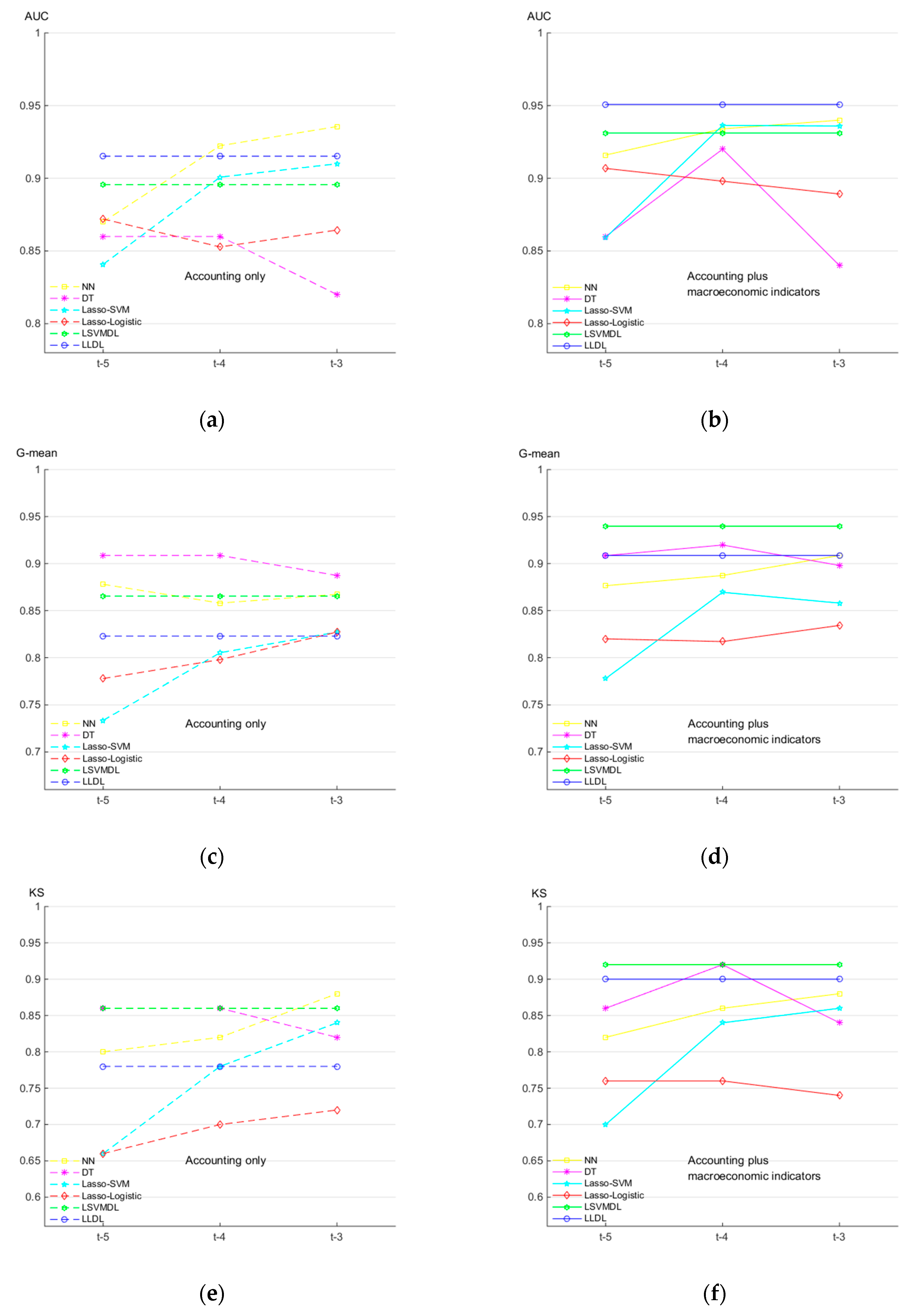
5.2.4. Comparison with Other Models

For the purpose of comparison, the prediction performances of the ex-ante models for the estimation of financial distress likelihood developed by the existing studies are shown in Table 5 and Table 6. The existing widely used ex-ante models include the neural network (NN), decision tree (DT), SVM, and logistic models estimated in different time periods of t − 3, t − 4, and t − 5, called t − 3 models, t − 4 models and t − 5 models. The construction of these three groups of models is similar to [7]. Let us take the construction of t − 5 model as example. For 10 financially distressed companies that received ST in 2012 and the selected 10 healthy companies until 2012 as a control group, their financial and macroeconomic data in 2007 (5 years before 2012) were collected. For 9 financially distressed companies that received ST in 2013 and the selected 9 healthy companies, their financial and macroeconomic data in 2008 (5 years before 2013) were collected. Similarly, for 17, 24, 26 financial distressed companies that receive the ST label respectively in 2014, 2015 and 2016 and the non-financial companies randomly selected at a 1:1 ratio in each year for matching with the ST companies, their data in 2009 (5 years before 2014), 2010 (5 years before 2015) and in 2011 (5 years before 2016) were collected. By using the labels of 172 companies and the data that were obtained 5 years prior to the year when the companies received the ST label, we construct t − 5 financial distress forecast models combined with a neural network (NN), decision tree (DT), SVM, and logistic regression. Similarly, t − 3 models and t − 4 models can be built. The data of financially distressed companies that received ST in 2017 and non-financial distressed companies were used to evaluate these models’ predicting performance.

As mentioned in the beginning of this section, three measures of prediction performances are reported in these two tables, namely, AUC, G-mean, and Kolmogorov–Smirnov statistics. In the above scenarios based on different time periods as well as division of the whole dataset, we compare respectively the predicting performance of those one-time window models (t − 3 models, t − 4 models and t − 5 models) including financial ratios only and financial ratios plus macroeconomic factors with our lasso–SVM-distributed lag (LSVMDL) model and lasso–logistic-distributed lag (LLDL). The prediction results are presented in Table 5 for the case of “financial ratios only” and Table 6 for the case of “financial ratio plus macroeconomic factors”.

In Table 5, panel A presents the predictive performances of NN, DT, lasso–SVM and lasso–logistic models including the original 43 financial ratios shown in Table 1 in the period t − 3 as predictors of financial distress status in period t, while the results in the last two columns are the performances of the two groups of distributed lag financial distress predicting models including the same original 43 financial ratios but in periods t − 3, t − 4 and t − 5, i.e., our models. Panel B and C of Table 5 present the prediction performance of the models used for comparison purposes estimated in t − 4 and t − 5, respectively. The results for our models retain the same values because these models include simultaneously the 3-year-, 4-year- and 5-year-lagged financial ratios.

The only difference between Table 5 and Table 6 is that all models, in addition to the 43 original accounting rations, incorporate 4 macroeconomic indicators in different time windows. For example, for time window t − 3, the NN, DT, lasso–SVM and lasso–logistic models include 3-year-lagged macroeconomic indicators shown in Table 2 in addition to the financial statement ratios shown in Table 1. The cases of time windows t − 4 and t − 5 are similar for these models. As for the LSVMDL and LLDL models, i.e., our models, they include 3-periods-lagged macroeconomic indicators in the time windows t − 3, t − 4 and t − 5 in addition to the accounting ratios.

From Table 5, the prediction accuracy of NN or DT is highest in the time windows t − 3 and t − 4; our models outperform the others in time window t − 5 for predicting accuracy. Generally speaking, the accuracy for time period t − 3 is relatively higher than the other two time periods for the NN, lasso–SVM and lasso–logistic models. Furthermore, the prediction results based on time period t − 3 are the most precise for NN when compared with other models in a single time period and even our models, which implies that the selected financial ratios in the period closer to the time of obtaining ST may contain more useful information for the prediction of financial distress, and may be applicable to NN. The AUC of 91.52% of the lasso–logistic-distributed lag model (LLDL) ranked second, close to the accuracy of 93.56% obtained by using NN. Therefore, the LLDL model should be competitive in terms of interpretability and accuracy in the case of “accounting ratio only”.

From Table 6, the prediction accuracy of all used models is higher than the results in Table 5. For example, the AUC, G-mean and KS of the NN model in time window t − 3 increases from 93.56%, 86.73% and 88.00% in Table 5 to 94.00%, 90.87% and 89.00% in Table 6, respectively. The changing tendency of the prediction accuracy is retained for the other models, including macroeconomic indicators in addition to the accounting ratios. All results in Table 6 indicate that the introduction of the macroeconomic variables can improve predictive performance of all used models for the purpose of comparison; the changes in macroeconomic conditions do affect the likelihood of financial distress risk. On the other hand, the LLDL model performs best with the AUC of over 95% when compared with the best NN (in time period t − 3, 94%), the best DT (in time period t − 4, 92.24%), the best lasso–SVM (in time period t − 4, 93.64%), the best lasso–logistic (in time period t − 5, 90.68%) and LSVMDL (93.12%). The LSVMDL model is the best performing model in terms of G-mean and KS statistics.

Figure 2 also shows the comparative results of the accuracy of the six models. The predictive performances of all the models including accounting ratios only, indicated by the dotted lines (a), (c) and (e) in Figure 2, are worse than the models including macroeconomic indicators as well as accounting ratios, which are illustrated by the solid lines (b), (d) and (f) in Figure 2. Figures (a) and (b), G-Mean for (c) and (d), and KS for (e) and (f) present AUC, G-mean and KS for all of the examined models, respectively. The models used for comparison, namely, NN, DT, lasso–SVM and lasso–logistic models, were those that yielded the highest accuracy based on the different time window dataset. For example, based on the results of panel (b), AUC of NN (the yellow solid line), DT (the pink solid line), and lasso–logistic (the red one) models are highest in time window t − 3, t − 4 and t − 5, respectively. We cannot conclude that the prediction results based on financial and macroeconomic data of one specific time window, e.g., t − 3 (see [7]), are the most accurate. However, from the results in (b), (d) and (f), our models, the LLDL or LSVMDL model incorporating financial and macroeconomic data in three consecutive time-windows, yielded relatively robust and higher prediction performances.

Put simply, the two groups of generalized distributed lag financial distress predicting models proposed by this paper outperform the other models in each time period, especially when the accounting ratios and macroeconomic factors were introduced into the models. We demonstrated that our models provide an effective way to deal with multiple time period information obtained from changes in accounting and macroeconomic conditions.

5.2.5. Discussion

Logistic regression and multivariate discriminant methods should be the most popular statistical techniques used in financial distress risk prediction modelling for different countries’ enterprise, e.g., American enterprises [1] and European enterprises [4,30,31], because of their simplicity, good predictive performance and interpretability. The main statistical approach involved in this study is logistic regression, but rather multivariate discriminant analysis, given that strict assumptions regarding normal distribution of explanatory variables are used in multivariate discriminant analysis. The results in this study conform that logistic regression models still perform well for predicting Chinese listed enterprises’ financial distress risks.

The major contribution to financial distress prediction literature made by this paper is that an optimally distributed lag structure of macroeconomic data in the multi-periods, in addition to financial ratio data, are imposed on the logistic regression model through minimizing loss function, and the heterogenous lagged effects of the factors in the different period are presented. The results unveil that financial indicators, such as total liabilities/total assets, sales revenue/total assets, and net cash flow from operating activities/total assets, tend to have a significant impact over relatively longer periods, e.g., 5 years before the financial crisis of a Chinese listed manufacturing company. This finding is in accordance with the recent research of [30,31] in that the authors claim the process of going bankrupt is not a sudden phenomenon; it may take as long as 5–6 years. In the very recent study of Korol et al. [30], the authors built 10 group models comprising 10 periods: from 1 year to 10 years prior to bankruptcy. The results in [30] indicate that a bankruptcy prediction model such as the fuzzy set model maintained an effectiveness level above 70% until the eighth year prior to bankruptcy. Therefore, our model can be extended through introducing more lagged explanatory variables, e.g., 6- to 8-year-lagged financial variables, which may bring a better distributive lag structure of explanatory variables and predicting ability of the models.

The findings of this study allow managers and corporate analysts to prevent financial crisis of a company by monitoring early changes in a few sensitive financial indicators and taking actions, such as optimizing the corporate’s asset structure, increasing cash flow and sales revenue, etc. They are also helpful for investors to make investment decision by tracking continuous changes in accounting conditions of a company of interest and predicting its risk of financial distress.

Another major contribution of this study is the confirmation of the importance of macroeconomic variables in predicting the financial distress of a Chinese manufacturing company, although scholars still argue about the significance of macro variables. For example, Kacer et al. [66] did not recommend the use of macro variables in the financial distress prediction for Slovak Enterprises, while Hernandez Tinoco et al. [4] confirmed the utilization of macro variables in the financial distress prediction for listed enterprises of the United Kingdom. The results in Section 5.2.4 of this study show that the prediction performance of all models (including both the models used for comparison and our own models) was increased when the macro variables were included in each model. The findings of this study allow regulators to tighten the supervision of Chinese listed companies when macroeconomic conditions change, especially in an economic downturn.

One of the main limitations of this study is that we limited the research only to the listed manufacturing companies. Both Korol et al. [28] and Kovacova [30] emphasized that the type of industry affects the risk of deterioration in the financial situation of companies. More specifically, distinguished by factors such as intensity of competition, life cycle of products, demand, changes in consumer preferences, technological change, reducing entry barriers into the industry and susceptibility of the industry to business cycles, different industries are at different levels of risk [28]. The manufacturing sector, which includes the metal, mining, automotive, aerospace and housing industries, is highly susceptible to demands, technological changes and macroeconomic conditions, thus making it at a high level of risk, while agriculture may be at a relatively low risk level. The risk parameter assigned to the service sector, including restaurants, tourism, transport and entertainment etc., has seen significant changes following the outbreak of the Coronavirus. Therefore, applicability and critique to our models for predicting financial distress risk of the companies operating in other industry and even other countries need to be further detected.

6. Conclusions

In this paper, we propose a new framework of a financial early warning system through introducing a distributed lag structure to be widely used in financial distress prediction models such as the logistic regression and SVM models. Our models are competitive when compared with the conventional financial distress forecast models, which incorporates data from only one-period of t − 3 or t − 4 or t − 5, in terms of predictive performance. Furthermore, our models are superior to the conventional one-time window financial distress forecast models, in which macroeconomic indicators of GDP growth, consumption level growth and unemployment rate, in addition to accounting factors, are incorporated. The empirical findings of this study indicate that the changes in macroeconomic conditions do have significant and continuous influence on the financial distress risk of a listed manufacturing company. This paper may provide an approach of examining the impacts of macroeconomic information from multiple periods and improving the predictive performance of financial distress models.

We implement feature selection to remove redundant factors from the original list of 43 potentially helpful ratios and their lags by introducing lasso penalty into the financial distress forecast logistic models with lags and SVM models with lags. Furthermore, we provide an ADMM algorithm framework that yields the global optimum for convex and the non-smooth optimization problem to obtain the optimal estimation for the coefficients of these financial distress forecast models with financial and macroeconomic factors and their lags. Results from the empirical study show that not only widely used financial indicators (calculated from accounting data), such as leverage ratio, ROE, ROA, and current liabilities/total liabilities, have significant influence on the financial distress risk of a listed manufacturing company, but also the indicators that are rarely seen in the existing literature, such as net profit attributable to shareholders of the parent company and net cash flow from operating activities/total assets, may play very important roles in financial distress prediction. The closer to the time of financial crisis, the more net profit attributable to shareholders of the parent company and net cash flow from operating activities may considerably decrease the financial distress risk. These research findings may provide more evidence for company managers and investors in terms of corporate governance or risk control.

The main limitation of this research is that we limited the research only to listed manufacturing companies. Sensitivity of financial distress models and suitability of both financial and macroeconomic variables to the enterprises that operate in other industries, e.g., service companies, need to be further discussed. On the other hand, given that the utilization of financial and macroeconomic variables in predicting the risk of financial distress of Chinese listed manufacturing companies is confirmed, we intend to continue the research toward the use of interaction terms of financial and macroeconomic variables in the context of the multiple period. Furthermore, the heterogeneous effect of changes in macroeconomic conditions on the financial distress risk of a company under different financial conditions can be discovered.

References

1. Altman, E.I. Financial ratios, discriminant analysis and the prediction of corporate bankruptcy. J. Financ. 1968, 23, 589–609. [Google Scholar] [CrossRef]
2. Lau, A.H.L. A five-state financial distress prediction model. J. Account. Res. 1987, 25, 127–138. [Google Scholar] [CrossRef]
3. Jones, S.; Hensher, D.A. Predicting firm financial distress: A mixed logit model. Account. Rev. 2004, 79, 1011–1038. [Google Scholar] [CrossRef]
4. Hernandez Tinoco, M.; Holmes, P.; Wilson, N. Polytomous response financial distress models: The role of accounting, market and macroeconomic variables. Int. Rev. Financ. Anal. 2018, 59, 276–289. [Google Scholar] [CrossRef] [Green Version]
5. Zmijewski, M.E. Methodological issues related to the estimation of financial distress prediction models. J. Account. Res. 1984, 22, 59–82. [Google Scholar] [CrossRef]
6. Ross, S.; Westerfield, R.; Jaffe, J. Corporate Finance; McGraw-Hill Irwin: New York, NY, USA, 2000. [Google Scholar]
7. Geng, R.; Bose, I.; Chen, X. Prediction of financial distress: An empirical study of listed Chinese companies using data mining. Eur. J. Oper. Res. 2015, 241, 236–247. [Google Scholar] [CrossRef]
8. Westgaard, S.; Van Der Wijst, N. Default probabilities in a corporate bank portfolio: A logistic model approach. Eur. J. Oper. Res. 2001, 135, 338–349. [Google Scholar] [CrossRef]
9. Balcaen, S.; Ooghe, H. 35 years of studies on business failure: An overview of the classic statistical methodologies and their related problems. Br. Account. Rev. 2006, 38, 63–93. [Google Scholar] [CrossRef]
10. Martin, D. Early warnings of bank failure: A logit regression approach. J. Bank. Financ. 1977, 1, 249–276. [Google Scholar] [CrossRef]
11. Liang, D.; Tsai, C.F.; Wu, H.T. The effect of feature selection on financial distress prediction. Knowl. Based Syst. 2015, 73, 289–297. [Google Scholar] [CrossRef]
12. Frydman, H.; Altman, E.I.; Kao, D.L. Introducing recursive partitioning for financial classification: The case of financial distress. J. Financ. 1985, 40, 269–291. [Google Scholar] [CrossRef]
13. Leshno, M.; Spector, Y. Neural network prediction analysis: The bankruptcy case. Neurocomputing 1996, 10, 125–147. [Google Scholar] [CrossRef]
14. Shin, K.S.; Lee, T.S.; Kim, H.J. An application of support vector machines in bankruptcy prediction model. Expert Syst. Appl. 2005, 28, 127–135. [Google Scholar] [CrossRef]
15. Sun, J.; Li, H. Data mining method for listed companies’ financial distress prediction. Knowl. Based Syst. 2008, 21, 1–5. [Google Scholar] [CrossRef]
16. Jiang, Y.; Jones, S. Corporate distress prediction in China: A machine learning approach. Account. Financ. 2018, 58, 1063–1109. [Google Scholar] [CrossRef] [Green Version]
17. Purnanandam, A. Financial distress and corporate risk management: Theory and evidence. J. Financ. Econ. 2008, 87, 706–739. [Google Scholar] [CrossRef]
18. Almamy, J.; Aston, J.; Ngwa, L.N. An evaluation of Altman’s Z-score using cash flow ratio to predict corporate failure amid the recent financial crisis: Evidence from the UK. J. Corp. Financ. 2016, 36, 278–285. [Google Scholar] [CrossRef]
19. Liang, D.; Lu, C.C.; Tsai, C.F.; Shih, G.A. Financial ratios and corporate governance indicators in bankruptcy prediction: A comprehensive study. Eur. J. Oper. Res. 2016, 252, 561–572. [Google Scholar] [CrossRef]
20. Scalzer, R.S.; Rodrigues, A.; Macedo, M.Á.S.; Wanke, P. Financial distress in electricity distributors from the perspective of Brazilian regulation. Energy Policy 2019, 125, 250–259. [Google Scholar] [CrossRef]
21. Altman, I.E.; Haldeman, G.R.; Narayanan, P. ZETATM analysis A new model to identify bankruptcy risk of corporations. J. Bank. Financ. 1977, 1, 29–54. [Google Scholar] [CrossRef]
22. Inekwe, J.N.; Jin, Y.; Valenzuela, M.R. The effects of financial distress: Evidence from US GDP growth. Econ. Model. 2018, 72, 8–21. [Google Scholar] [CrossRef]
23. Ohlson, J. Financial ratios and the probabilistic prediction of bankruptcy. J. Account. Res. 1980, 18, 109–131. [Google Scholar] [CrossRef] [Green Version]
24. Hillegeist, S.; Keating, E.; Cram, D.; Lundstedt, K. Assessing the probability of bankruptcy. Rev. Account. Stud. 2004, 9, 5–34. [Google Scholar] [CrossRef]
25. Teresa, A.J. Accounting measures of corporate liquidity, leverage, and costs of financial distress. Financ. Manag. 1993, 22, 91–100. [Google Scholar]
26. Shumway, T. Forecasting bankruptcy more accurately: A simple hazard model. J. Bus. 2001, 74, 101–124. [Google Scholar] [CrossRef] [Green Version]
27. Hosaka, T. Bankruptcy prediction using imaged financial ratios and convolutional neural networks. Expert Syst. Appl. 2019, 117, 287–299. [Google Scholar] [CrossRef]
28. Korol, T. Dynamic Bankruptcy Prediction Models for European Enterprises. J. Risk Financ. Manag. 2019, 12, 185. [Google Scholar] [CrossRef] [Green Version]
29. Gregova, E.; Valaskova, K.; Adamko, P.; Tumpach, M.; Jaros, J. Predicting Financial Distress of Slovak Enterprises: Comparison of Selected Traditional and Learning Algorithms Methods. Sustainability 2020, 12, 3954. [Google Scholar] [CrossRef]
30. Kovacova, M.; Kliestik, T.; Valaskova, K.; Durana, P.; Juhaszova, Z. Systematic review of variables applied in bankruptcy prediction models of Visegrad group countries. Oeconomia Copernic. 2019, 10, 743–772. [Google Scholar] [CrossRef] [Green Version]
31. Kliestik, T.; Misankova, M.; Valaskova, K.; Svabova, L. Bankruptcy Prevention: New Effort to Reflect on Legal and Social Changes. Sci. Eng. Ethics 2018, 24, 791–803. [Google Scholar] [CrossRef]
32. López, J.; Maldonado, S. Profit-based credit scoring based on robust optimization and feature selection. Inf. Sci. 2019, 500, 190–202. [Google Scholar] [CrossRef]
33. Maldonado, S.; Pérez, J.; Bravo, C. Cost-based feature selection for Support Vector Machines: An application in credit scoring. Eur. J. Oper. Res. 2017, 261, 656–665. [Google Scholar] [CrossRef] [Green Version]
34. Li, J.; Qin, Y.; Yi, D. Feature selection for Support Vector Machine in the study of financial early warning system. Qual. Reliab. Eng. Int. 2014, 30, 867–877. [Google Scholar] [CrossRef]
35. Duffie, D.; Saita, L.; Wang, K. Multi-Period Corporate Default Prediction with Stochastic Covariates. J. Financ. Econ. 2004, 83, 635–665. [Google Scholar] [CrossRef] [Green Version]
36. Greene, W.H.; Hensher, D.A.; Jones, S. An Error Component Logit Analysis of Corporate Bankruptcy and Insolvency Risk in Australia. Econ. Rec. 2007, 83, 86–103. [Google Scholar]
37. Figlewski, S.; Frydman, H.; Liang, W.J. Modeling the effect of macroeconomic factors on corporate default and credit rating transitions. Int. Rev. Econ. Financ. 2012, 21, 87–105. [Google Scholar] [CrossRef]
38. Tang, D.Y.; Yan, H. Market conditions, default risk and credit spreads. J. Bank. Financ. 2010, 34, 743–753. [Google Scholar] [CrossRef] [Green Version]
39. Chen, C.; Kieschnick, R. Bank credit and corporate working capital management. J. Corp. Financ. 2016, 48, 579–596. [Google Scholar] [CrossRef]
40. Jermann, U.; Quadrini, V. Macroeconomic effects of financial shocks. Am. Econ. Rev. 2012, 102, 238–271. [Google Scholar] [CrossRef] [Green Version]
41. Carpenter, J.N.; Whitelaw, R.F. The development of China’s stock market and stakes for the global economy. Annu. Rev. Financ. Econ. 2017, 9, 233–257. [Google Scholar] [CrossRef] [Green Version]
42. Hua, Z.; Wang, Y.; Xu, X.; Xu, X.; Zhang, B.; Liang, L. Predicting corporate financial distress based on integration of support vector machine and logistic regression. Expert Syst. Appl. 2007, 33, 434–440. [Google Scholar] [CrossRef]
43. Li, H.; Sun, J. Hybridizing principles of the Electre method with case-based reasoning for data mining: Electre-CBR-I and Electre-CBR-II. Eur. J. Oper. Res. 2009, 197, 214–224. [Google Scholar] [CrossRef]
44. Cao, Y. MCELCCh-FDP: Financial distress prediction with classifier ensembles based on firm life cycle and Choquet integral. Expert. Syst. Appl. 2012, 39, 7041–7049. [Google Scholar] [CrossRef]
45. Shen, F.; Liu, Y.; Wang, R. A dynamic financial distress forecast model with multiple forecast results under unbalanced data environment. Knowl. Based Syst. 2020, 192, 1–16. [Google Scholar] [CrossRef]
46. Gasparrini, A.; Armstrong, B.; Kenward, M.G. Distributed lag non-linear models. Stat. Med. 2010, 29, 2224–2234. [Google Scholar] [CrossRef] [Green Version]
47. Gasparrini, A.; Scheipl, B.; Armstrong, B.; Kenward, G.M. Penalized Framework for Distributed Lag Non-Linear Models. Biometrics 2017, 73, 938–948. [Google Scholar] [CrossRef] [PubMed]
48. Wilson, A.; Hsu, H.H.L.; Chiu, Y.H.M. Kernel machine and distributed lag models for assessing windows of susceptibility to mixtures of time-varying environmental exposures in children’s health studies. arXiv 2019, arXiv:1904.12417. [Google Scholar]
49. Nelson, C.R.; Schwert, G.W. Estimating the Parameters of a Distributed Lag Model from Cross-Section Data: The Case of Hospital Admissions and Discharges. J. Am. Stat. Assoc. 1974, 69, 627–633. [Google Scholar] [CrossRef]
50. Hammoudeh, S.; Sari, R. Financial CDS, stock market and interest rates: Which drives which? N. Am. J. Econ. Financ. 2011, 22, 257–276. [Google Scholar] [CrossRef]
51. Lahiani, A.; Hammoudeh, S.; Gupta, R. Linkages between financial sector CDS spreads and macroeconomic influence in a nonlinear setting. Int. Rev. Econ. Financ. 2016, 43, 443–456. [Google Scholar] [CrossRef] [Green Version]
52. Almon, S. The distributed lag between capital appropriations and expenditures. Econometrica 1965, 33, 178–196. [Google Scholar] [CrossRef]
53. Dominici, F.; Daniels, M.S.L.; Samet, Z.J. Air pollution sand mortality: Estimating regional and national dose—Response relationships. J. Am. Stat. Assoc. 2002, 97, 100–111. [Google Scholar] [CrossRef]
54. Wooldridge, J.M. Econometric Analysis of Cross Section and Panel Data; MIT Press: Cambridge, MA, USA, 2010. [Google Scholar]
55. Park, H.; Sakaori, F. Lag weighted lasso for time series model. Comput. Stat. 2013, 28, 493–504. [Google Scholar] [CrossRef]
56. Glowinski, R.; Marroco, A. Sur l’approximation, par éléments finis d’ordre un, et la résolution, par pénalisation-dualité d’une classe de problèmes de Dirichlet non linéaires. ESAIM Math. Model. Numer. 1975, 9, 41–76. [Google Scholar] [CrossRef]
57. Dantzig, G.; Wolfe, J. Decomposition principle for linear programs. Oper. Res. 1960, 8, 101–111. [Google Scholar] [CrossRef]
58. Hestenes, M.R. Multiplier and gradient methods. J. Optim. Theory. Appl. 1969, 4, 302–320. [Google Scholar] [CrossRef]
59. Chambolle, A.; Pock, T. A first-order primal-dual algorithm for convex problems with applications to imaging. J. Math. Imaging Vis. 2011, 40, 120–145. [Google Scholar] [CrossRef] [Green Version]
60. Boyd, S.; Parikh, N.; Chu, E.; Peleato, B.; Eckstein, J. Distributed Optimization and Statistical Learning via the Alternating Direction Method of Multipliers. Found. Trends. Mach. Learn. 2011, 3, 1–122. [Google Scholar] [CrossRef]
61. Mangasarian, O.L. A finite Newton method for classification. Optim. Methods Softw. 2002, 17, 913–929. [Google Scholar] [CrossRef]
62. Shon, T.; Moon, J. A hybrid machine learning approach to network anomaly detection. Inf. Sci. 2007, 177, 3799–3821. [Google Scholar] [CrossRef]
63. Liu, D.; Qian, H.; Dai, G.; Zhang, Z. An iterative SVM approach to feature selection and classification in high-dimensional datasets. Pattern Recognit. 2013, 46, 2531–2537. [Google Scholar] [CrossRef]
64. Tiwari, R. Intrinsic value estimates and its accuracy: Evidence from Indian manufacturing industry. Future Bus. J. 2016, 2, 138–151. [Google Scholar] [CrossRef] [Green Version]
65. Shanker, M.; Hu, M.Y.; Hung, M.S. Effect of data standardization on neural network training. Omega Int. J. Manag. Sci. 1996, 24, 385–397. [Google Scholar] [CrossRef]
66. Kacer, M.; Ochotnicky, P.; Alexy, M. The Altman’s revised Z’-Score model, non-financial information and macroeconomic variables: Case of Slovak SMEs. Ekon. Cas. 2019, 67, 335–366. [Google Scholar]
Figure 1. (a,b) are the Cross-validation performances that result from applying lasso–logistic-distributed lag regression to the listed manufacturing companies’ data with various values of λ.
Mathematics 08 01275 g001
Figure 2. Predictive performance of NN, DT, lasso–SVM, and lasso–logistic models on three different time window datasets, respectively, and our models on three consecutive time window datasets, evaluated by AUC for (a) and (b), G-Mean for (c) and (d), and KS for (e) and (f).
Mathematics 08 01275 g002