Considering Random Factors in Modeling Complex Microeconomic Systems

Abstract

Within the framework of a model describing real-functioning association of three enterprises, numerical calculations of economic dynamics parameters considering fluctuating market demand for the goods were performed. A methodology was suggested for approximated consideration of both seasonal and random demand fluctuations at the market of textile garments; the main steps of the suggested methodology were described. The main exogenous random factors within this model include, as stated above, the volume of market demand for the goods produced by the enterprises of the group. The basic volume of market demand is considered at the average actual level according to the results of the enterprises’ analysis, and additionally we take into account the influence of non-price factors, such as random changes in the consumers’ tastes, consumers’ income, and other random factors on the market demand. By volume of market demand, we consider the total amount of goods produced by the enterprises of the group that all consumers are willing and able to purchase at a specific price in a marketplace. The calculations were made based on actual values of external economic parameters, such as labor cost, product prices, etc. Influence of the market demand fluctuations on the companies’ activity has been illustrated both numerically and graphically, allowing the analysis of the impact of exogenous parameters on the companies output and profits. The suggested approach creates a basis for further analysis of the impact of random factors of a similar nature, i.e., stochastic shocks related to the level of interest rates, shifts and turnabouts in the social environment, as well as the market transformations due to annual/seasonal epidemics.

1. Introduction

Analysis of companies and associations of companies acting as complex economic systems is an important instrument of management. Defining such systems’ potential and forecasting their activity can be a basis for grounded managerial decisions and serve as an instrument for controlling company’s activity. Such characteristics of complex economic systems, such as cohesiveness, dynamism, uncertainty, correlation with environment, etc., should be taken into account.

Economic modeling methods enable the consideration of special aspects of complex economic systems, serving as tools for factual information systematization, determining and rendering interrelations between different variables, generalizing results of economic analysis, and defining optimal managerial decisions. Modeling is an instrument for many areas of scientific research, so it has also been important for economics. Mathematic modeling, constantly advancing, shaping up, and reflecting basic needs of contemporary informational society, is one of the necessary tools for processing economic information.

Mathematical modeling is a powerful and flexible means of research for various models of real systems’ economic dynamics, study of their properties, and reaction on changes of internal parameters and external conditions of activity. In particular, performing numerical calculations provides sufficient evidence of the obtained results, simplification of data analysis, and optimal decisions finding. Efficient managerial decisions that result in increasing business value can be achieved by: modularizing the business into units, understanding the services provided by these units, and analyzing interrelationships amongst them [1], and modeling such relationships.

Modeling of complicated systems and processes, in particular in the area of production, in the markets of goods and services, securities, and study of other economic phenomena and processes, is about the only method of quantitative prognostication. However, notwithstanding the business model definition, not a single model is structurally identical to the object of study. Normally, for different reasons, there are certain factors of influence, random factors on the investigated system, that remain beyond the scope of analysis. Therefore, the results of their impact cannot be directly taken into account by means of certain functions. Indirect influence of random factors can be represented by means of variables that show stochastic function dependency upon time. A stochastic process, thus, is a probability model that describes evolution of a complicated system evolving randomly in time.

Building a system of equations that describe dynamics of the system parameters is the issue for many different economic theory aspects. Forecasting with the help of a mathematic-economic model is based on the structural and functional analysis of organization or its divisions, taking into account the influence of external environment and reflecting its business strategy [2]. In particular, in our works [3,4], a determined mathematical model of dynamics for the system of three associated enterprises was built. Certain enterprises of light industry were examined, and equations that describe dynamics of the system contained the real values of basic parameters and descriptions of the system [5]. Such a model allows us to carry out an imitation of the system function and develop a prognosis of its development in the chosen fixed conditions.

Building a simulation mathematical model of a dynamic economic system is of material interest, if its operating conditions are stochastic, id est, at presence of random parameters in the environment [6,7]. Studying properties of such models [8] helps with understanding the nature and consistent pattern of the economic system variance, provides the grounds for decisions regarding the choice of optimal development strategy, and allows the forecast of consequences of management decisions. An important aim of modeling is prognosis of endogenous parameters, and characteristics of the system determined in the model.

Parameters of companies’ function can bring in quality changes into their activity and thus impact the business value. Such parameters are indexes of competition and the operating environment that an enterprise is functioning in, say, price level (both for inputs and final products), technology characteristics, certain performance parameters of competitors (market concentration, industry profitability indexes, assets turnover, and level of costs), suppliers characteristics (amount of suppliers and their concentration), consumers indicators (preferences, purchasing power, price elasticity of demand, seasonality [9,10], and other demand fluctuations); and also general economic, political, legal, and other parameters of the environment, such as the rate of inflation, unemployment, tax and loan rates, trade policy of the state, etc.

Competitive environment is dynamic according to features such as rates, depth, and scale of changes at the markets. Actually, any influences of the environment on organizations’ activity are characterized by vagueness and can make quantitative and qualitative alterations.

For building an adequate model, it is necessary to investigate influence of a number of interrelated factors. Traditional methods of the determined factor analysis are often not in connection enough with the limited nature of their possibilities, insufficiency of the information support, etc. The necessity of wider use of stochastic factor analysis methods arises, which, unlike the strictly regulated methods of the determined analysis that are based on functional dependence of effective index of a factor, give an opportunity to take into account influence of the totality of factors that carry probabilistic, indefinite character.

Stochasticity is one of the properties of environment for economic systems, such as enterprises. As every organization is an open system, it is influenced by the environment. Such influences can have unforeseeable character (in particular force-majeure circumstances) and result in out-of-control changes in the activity of an organization. Considering the impact of random exogenous factors is an important element of economic analysis and prognostication for certain types of tasks.

Traditionally, stochastic analysis is applied in such cases, where the most typical tasks of economic analysis include:

• studying the existence of relations between functions and factors, and their closeness;
• classification of the economic phenomena factors;
• defining analytical forms of interrelation between the studied phenomena;
• determining the parameters of indexes’ periodic fluctuations conformity/law;
• study of quantitative changes of indexes/functions due to the influence of factors;
• economic interpretation of the obtained analytical dependences.

The methods of stochastic factor analysis include regressive, cross-correlation, component, multidimensional, and other types of analysis.

There are a number of modelling approaches presented in contemporary publications with accents made on studying the behavior of random variables, or particularly the mechanics of demand fluctuations [11,12]. Our work presents a practical application of random factors impact analysis related to a commonly applied structure of cooperation between production and sales units, which gives a basis for solving a broad spectrum of tasks within similar economic systems. It allows the programming of different changes in the variables having influence on the companies’ activity, and assessment of the group financial results as an outcome [13,14].

2. Model Building and Testing

In the previous works mentioned above, we presented a general mathematic model describing economic dynamics of three associated enterprises. The model includes exogenous (external) parameters, including market demand for the good, as well as endogenous (internal) parameters. The task of modeling investigates evolution of endogenous variables depending on the behavior of external factors. The task of forecasting activity for textile companies was addressed in a number of works [15,16,17], including studies related to general market dynamics [18,19,20] and search of synergetic relations [21]. The whole model presented in our previous works together, with the study of random factors described in the current article, covers all main economic aspects of production-and-sales group operations [22,23,24].

The general model [5] will be applied here for a special case— an actual enterprises’ association, functioning in the area of confectionary production and sales, including a Danish management, logistics, and sales company, “Miltex”; Ukrainian production factory, “Mriya”; and Polish production factory, “Emitex”. Economic parameters of the mentioned companies were considered.

In this particular case, the number of enterprises described in the model is n = 3. The indexes of enterprises: of production enterprises, “Mriya” is i = 1, and “Emitex”-i = 2; sales enterprise, “Miltex” (generating and placing orders) is i = 3.

Activity of the enterprise “Mriya” is currently at the stage of growth, while “Miltex” is at the stage of maturity. The market where “Mriya” is functioning is fragmented, and the company share is not significant. The market of “Miltex” is not fragmented, and the company share is significant.

In this case, association of the companies would be consistent according to a functional principle, providing vertical integration between the partnering companies. In this case, association of the companies would be consistent according to a functional principle, providing vertical integration between the partnering companies. Value chain strategies within this particular industry, as well as in similar markets, are constantly in the making. Successful ones rarely remain competitive for long [25], thus, our aim is adding to the general study of successful competitive strategies.

The purposes set by each of the parties are as follows:

• For enterprises 1 and 2: economy on scale due to vertical integration; benefits from access to resources (financial, material, technical, and also non-material), with the aim of strengthening financial status and technological upgrade of the enterprise; load leveling of production capacities during a year; transfer of organizational, production, and sales knowledge; use of existent practice of research and development (RnD) and production; and use of partner’s distribution trade mark in sales.
• For enterprise 3: possibility to exploit comparative advantages; risks distribution; potential advantages from entering new market with lower competition; using growth potential of the less mature market; economy on scale due to vertical integration; balancing production costs; common use of non-material resources, such as transfer of knowledge and experience; access to comparatively cheaper resources; and decrease of production costs.

The frames of the model calculations were performed for defining basic economic indicators of the enterprises. Participants’ activity, in particular, estimating the influence of changes in factors such as production volume and level of reinvestment and discounting, and changes of these factors were pre-defined. In this work, we will return to estimating the influence of these factors. However, considering random influences on the basic parameters allows the investigation of the dynamics of the system in a stochastic model.

The aim of this work is to develop and apply methodology considering variable and random factors for planning production capacity and to examine their influence on the basic economics parameters of the system.

The basic variables used for describing the system status are:

• $P_t^{\left(i\right)}$: retained earnings (accrued profits) over t months for each of the enterprises $i,\left(i=1,2,3\right)$, where i is the index of the enterprises;
• $K_t^{\left(i\right)}$: own accrued capital of the enterprise, $i;$
• $K{A}_t^{\left(i\right)}$: accrued invested (accepted) capital over t months from enterprise $3 \mathrm{to}\mathrm{enterprise} i,\left(i=1,2\right);$
• $Q_t^{\left(i\right)}$: level of output by production enterprises in month t (total output from the beginning of activity to the end of month t),$i=1,2$.

In descriptions of dynamics of the system, one may use recurrent or differential equations. For this particular purpose, we introduced some additional variables as functions of the abovementioned:

• $N{P}_t^{\left(i\right)}$: net profit of the enterprise $i,\left(i=1,2,3\right)$ in month t, not considering depreciation and amortization;
• $KPar{t}_t^{\left(i\right)}$: part of the enterprise’s 3 net profit, invested into the capital of enterprise $i,\left(i=1,2\right)$;
• $Npar{t}_t^{\left(3\right)}$: part of the enterprise’s 3 net profit remaining, after investing to the capital of other enterprises.

We build a 12-dimensional column vector:$\overline{X}\left(t\right)={\left\{P_t^{\left(i\right)},K_t^{\left(i\right)},K{A}_t^{\left(i\right)},Q_t^{\left(i\right)}\right\}}^T≣\left\{X_j^{\left(i\right)}\left(t\right)\right\},t=k·1month;i-1,2,3;j=1,2,3,4;k=1,2,3,\dots$

The column vector, $X\left(t\right)$, describes economic status and results of activity for each of the enterprises in month t. Components, $X_{j }^{\left(i\right)}$, of this vector are time-dependent values.

We should also consider the influence of exogenous economic factors on the system dynamics, such as product prices, wages, tax rate, level of some fixed costs, etc:

• $v_t^{(i)}$: transfer price (the price for which the production enterprise is selling its products to the sales enterprise within the group);
• $p_t{}^{(i)}$: the product sales price;
• $f_t^{(i)}$: monthly fixed general administrative expenses;
• $f{s}_t^{(i)}$: monthly fixed marketing and sales expenses;
• $s{c}_t^{(i)}$: variable unit sales costs;
• $l_t^{(i)}$: labor unit costs;
• $L_t^{(i)}$: number of direct production personnel at the enterprise;
• ${\eta }_t^{(i)}$: coefficient characterizing capital and labor productivity;
• ${\alpha }_t^{(i)}$: rate of profit reinvestment into the enterprise’s capital;
• ${\beta }_t^{\left(i\right)}$: rate of depreciation.

3. Results

3.1. Level of Production Orders, Income, and Investments

During conjoint activity of the enterprises, their total production output (production orders) is split by the sales enterprise between the production enterprises based on the level of their production costs. Efficiency of each production enterprise activity is estimated here as a parameter proportional to its relative (comparing to the total of two production enterprises) production capacity. Herewith, the levels of ancillary quantities, $Qor{d}^{\left(i\right)},Qma{x}^{\left(i\right)},i=1,2$, are considered, i.e., for enterprise 1, the level of quantity, $Qor{d}^{\left(1\right)}$, is:

$$Qor{d}^{\left(1\right)}\left(t,kr,ks\right)=Dm\left(t,kr,ks\right) ·\frac{Qma{x}^{\left(1\right)}\left(t\right)·{\nu }^{\left(2\right)}}{Qma{x}^{\left(2\right)}\left(t\right)·{\nu }^{\left(1\right)}+Qma{x}^{\left(1\right)}·{\nu }^{\left(2\right)}},$$

(1)

where $Qma{x}^{\left(i\right)}\left(t\right)$ is the maximum possible production capacity of the enterprise (defined based on the total amount of the capital, labor, and efficiency of the enterprise inputs). The function of maximum production capacity relates to a modified Cobb–Douglas production function [26]:

$$Qma{x}^{\left(i\right)}\left(t\right)={\eta }^{\left(i\right)}·{\left(K{A}_{t }^{\left(i\right)}+K_t^{\left(i\right)}\right)}^{\lambda 1}·L^{\left(i\right)}{}^{\lambda 2},$$

(2)

where λ1, λ2 are parameters characterizing efficiency of the enterprise inputs (capital and labor); λ1 + λ2 = 1; λ1, λ2 > 0.

Production output for enterprise i (i = 1, 2) is planned equal to the lesser of the two described values, $Qor{d}^{\left(i\right)}\left(t,kr,ks\right), Qma{x}^{\left(i\right)}\left(t\right)$.

Each of the enterprises possesses an initial amount of capital depreciated at given rate, which may increase due to reinvestments of the net profit and is calculated as the sum of starting own capital and reinvested net profit during the period of activity. Increase of the enterprise own capital equals

$$K_{t+1}^{\left(i\right)}=K_t^{\left(i\right)}+\frac{{\alpha }^{\left(i\right)}}{1-{\alpha }^{\left(i\right) }}N{P}_t{}^{\left(i\right)}-{\beta }^{\left(i\right)}{K}_t^{\left(i\right)},$$

(3)

where ${\alpha }^{\left(i\right)}$ is the rate of reinvestment of the net profit into productive capital of the enterprise i, ${\beta }^{\left(i\right)}$ is the rate of depreciation of the capital of enterprise i per month, and $N{P}_t{}^{\left(i\right)}$ is the amount of net profit of enterprise i per month t:

$$N{P}_t{}^{\left(i\right)}=\left[Q_t{}^{\left(i\right)}\left({\nu }^{\left(i\right)}-l^{\left(i\right)}\right)-f^{\left(i\right)}\right]·\left(1-{\alpha }^{\left(i\right)}\right)\frac{K_t^{\left(i\right)}}{K{A}_t^{\left(i\right)}+K_t^{\left(i\right)}}$$

(4)

Initial amount of the enterprises’ capital reflects purely the level of its own capital. During the enterprises’ conjoint activity, the sales enterprise (acting as a client at the beginning) becomes also a strategic partner, investing its own resources into the capital of the production enterprises. Increase of the accepted (invested) capital at the beginning of the month t+1 for production enterprises (union members) is calculated according to the formula:

$$\Delta K{A}_t^{\left(i\right)}=K{A}_{t+1}^{\left(i\right)}-K{A}_t^{\left(i\right)}=Kpar{t}_t^{\left(i\right)}-{\beta }^{\left(i\right)}K{A}_t^{\left(i\right)},$$

(5)

where $Kpar{t}_t^{\left(i\right)}$ is the share of the sales enterprise’s net profit invested into the capital of production enterprise i in month t.

Amount of investments from the side of the strategic partner into the capital of production enterprises, depends on the maximally permissible share of the strategic partner in the capital of the accepting production enterprise for the previous month and the total amount of net profit of the sales enterprise, which is the source of reinvestments. Amounts of investments by the sales enterprise into the capital of enterprise i equals

$$Kpar{t}_t^{\left(i\right)}=\min \left(Si{0}_t^{\left(i\right)},Si{1}_t^{\left(i\right)}\right),$$

(6)

where $Si{0}_t^{\left(i\right)}$ is the amount of investment into the capital of enterprise i, defined as the part of total investments in the current month, proportional to the relative capital profitability/return on equity:

$$Si{0}_t^{\left(i\right)}={\alpha }^{\left(i\right)}\frac{N{P}_t{}^{\left(i\right)}}{1-{\alpha }^{\left(i\right)}}R{E}_t^{\left(i\right)}; Si{1}_t^{\left(i\right)}=\left(1-{\beta }^{\left(i\right)}\right)\left\{\frac{1}{1-{\mu }^{\left(i\right)}}{K}_t^{\left(i\right)}-K{A}_t^{\left(i\right)}\right\}.$$

(7)

$R{E}_t^{\left(i\right)}$, or relative profitability of the production enterprises’ capital (i = 1,2):

$$R{E}_t^{\left(i\right)}=\frac{N{P}_t^{\left(i\right)}/K_t^{\left(i\right)}}{{{\displaystyle \sum }}_{j=2,3}\left[\raisebox{1ex}{$N{P}_t^{\left(j\right)}/K_t^{\left(j\right)}$}\!\left/ \!\raisebox{-1ex}{$K_t^{\left(j\right)}$}\right.\right]}.$$

$Si{1}_t^{\left(i\right)}$ is the amount of investments, which allows the production enterprise i to remain owner of the main share of the total capital, considering the described system of reinvestments.

${\mu }^{\left(i\right)}$ is the allowable relative share of the accepted capital in total capital value (defined by the enterprise management).

Net profit of the sales enterprise, $N{P}_t^{\left(3\right)}$, equals the sum of the income from sales and income from financial investments (participation in the capital of the production enterprises), decreased by the sum of fixed monthly costs and variable costs. The latter includes costs related to the sales of goods, $s{c}^{\left(3\right)}$; transport costs, $t{r}_t^{\left(1\right)} \mathrm{and}t{r}_t^{\left(2\right)}$; costs for delivery of goods from production enterprises to the sale enterprise; and costs of the purchase of the goods at the transfer prices:

$$N{P}_t^{\left(1\right)}=\left(p^{\left(3\right)}-s{c}^{\left(3\right)}\right)·\left(Q_t^{\left(1\right)}+Q_t^{\left(2\right)}\right)+{\displaystyle \sum }_{i=1,2}P{K}_t^{\left(i\right)}-f{s}_t^{\left(i\right)}-{\displaystyle \sum }_{i=1,2}\left({\nu }^{\left(i\right)}+t{r}_t^{\left(i\right)}\right)Q_t^{\left(i\right)},$$

(8)

where $P{K}_t^{\left(i\right)}$ is the income of the sales enterprise from financial investments into the capital of enterprise i, i = 1,2:

$$P{K}_{t }^{\left(i\right)}=N{P}_t^{\left(i\right)}·\frac{K{A}_t^{\left(i\right)}}{K{A}_t^{\left(i\right)}+K_t^{\left(i\right)}}.$$

(9)

Retained earnings of the sales enterprise equals the difference between its net profit and the amount of investments into the capital of production enterprises. Repayment of the financial profit on investments by the accepting enterprises will be performed after all their own costs are covered. Thus, the investor is partly involved in covering the costs of production enterprises. Total amount of the investments into the capital of production enterprises is related to the total group profit, therefore, each production enterprise is interested in total group success. That is one of preconditions of synergy [27] in the present group structure.

For building the model as a system of differential equation, we assume that time (t) is changing discretely in a step of 1 month: $\Delta \mathrm{t}=1$ month. Formally going to $\Delta \mathrm{t}\to 0$, we obtain a first-order system of nonlinear differential equations.

We suppose that each of these factors is slightly dependent on time within the scale of the group activity, therefore, the equations describing system dynamics, we write as

$$\frac{d{X}_j^{\left(i\right)}}{dt }=F_j^{\left(i\right)}, i=1,2,3; j=1,2,3,4.$$

Considering endogenous parameters as components $x_i=1, 2, \dots$ of a certain vector $\overline{x}$, i.e.,

$x_1=P_1, x_2=K_1$, etc., this system of equations may be written as

$$\frac{d{x}_i}{dt}=f_i\left( \overline{x}\right) \to \frac{d{P}_i}{dt}=F_i\left(P_1,P_2,K_1,K_2\right), \frac{{\mathrm{dK}}_{\mathrm{i}}}{\mathrm{dt}}={\mathrm{G}}_{\mathrm{i}}\left({\mathrm{P}}_1,{\mathrm{P}}_2,{\mathrm{K}}_1,{\mathrm{K}}_2\right).$$

(10)

The functions, $F_j^{\left(i\right)}$, depend on the elements of the column vector, $\left\{X_j^{\left(i\right)}\right\}$, and on the mentioned above factors.

In our previous works, as mentioned above, adduced calculations were implemented in recurrent equations (not presented here due to their length) describing dynamics of the considered economic system. The equations were simplified to linearized differential equations, and investigation of the dependence between the system’s solutions stability, and enterprises’ activity mode on different factors and the components of the column vector were performed, providing a possibility of establishing intervals of their optimum and undesirable values.

At the same time, certain elements of the investigation were performed in a simplified manner. In particular, it concerns the investigation of the mode of the enterprises’ activity, given some fluctuations in production output.

3.2. Considering Demand Fluctuations

3.2.1. Seasonal Fluctuations

Economic forecasting requires the inclusion of the study of trendy, seasonal, cyclical, and random aspects [28,29]. Influence of consumer demand of similar structure on the results of organization activity was investigated in [30,31]. Production and sales output level forecasting has been studied in [29,30,31,32].

The main exogenous random factors within this model include, as stated above, the volume of market demand for the goods produced by the enterprises of the group and the cash flow discount rate. The basic volume of market demand is considered at the average actual level according to the results of the enterprises analysis. Additionally, we take into account the influence of non-price factors, such as random changes in consumers’ tastes, consumers’ income, and other random factors on the market demand [33]. Using the volume of market demand, we consider the total amount of goods produced by the enterprises of the group that all consumers are willing and able to purchase at a specific price in a marketplace [34,35].

We are using the term of guaranteed monthly demand, D(t), as the maximum volume of output that can be sold in month t completely. Let us assume that the amount of production and amount of sales are equal in each given month.

We also make the following assumptions regarding market demand:

• Initial monthly volume of the market demand equals the average actual level, defined as the result of preliminary enterprises analysis.
• There is a general upward trend in the market volume of 15% annually; we make such an assumption based on analysis of the previous years’ data, as well as active marketing policy of the group.
• The fluctuations of market demand have a seasonal character, such as periodic increase and periodic decrease in certain months during the year.
• The level of market demand does not depend on the price level. We assume that the group is functioning at a market of perfect competition and is a price taker (does not essentially influence the price).
• Besides the (rather predictable) seasonal fluctuations, the level of market demand is also influenced by random external factors.
• The level of market demand for a certain period is the indicator of the maximum production output of the goods for this period, there is no work-in-progress considered.

According to these assumptions, the monthly demand for the goods is the sum of the mentioned above upward trend, component D(t) (t—number of months of the group activity), which we will call guaranteed demand, and variable components related to seasonal and random demand fluctuations.

We set the following approximated form for the guaranteed demand:

$$D\left(t\right)=D0\left(1+kmax\left(1-exp\left(-\delta \frac{t}{Tm}\right)\right)\right),$$

(11)

where D0 is the initial monthly demand for the goods; Tm is time (months), during which monthly demand is reaching 95% of the maximum monthly demand, Dmax, at the given market segment; $kmax=\frac{Dmax}{D0}$ is the coefficient of maximum demand growth; and $\delta =-ln\left(0.05+\frac{1}{kmax}\right)$.

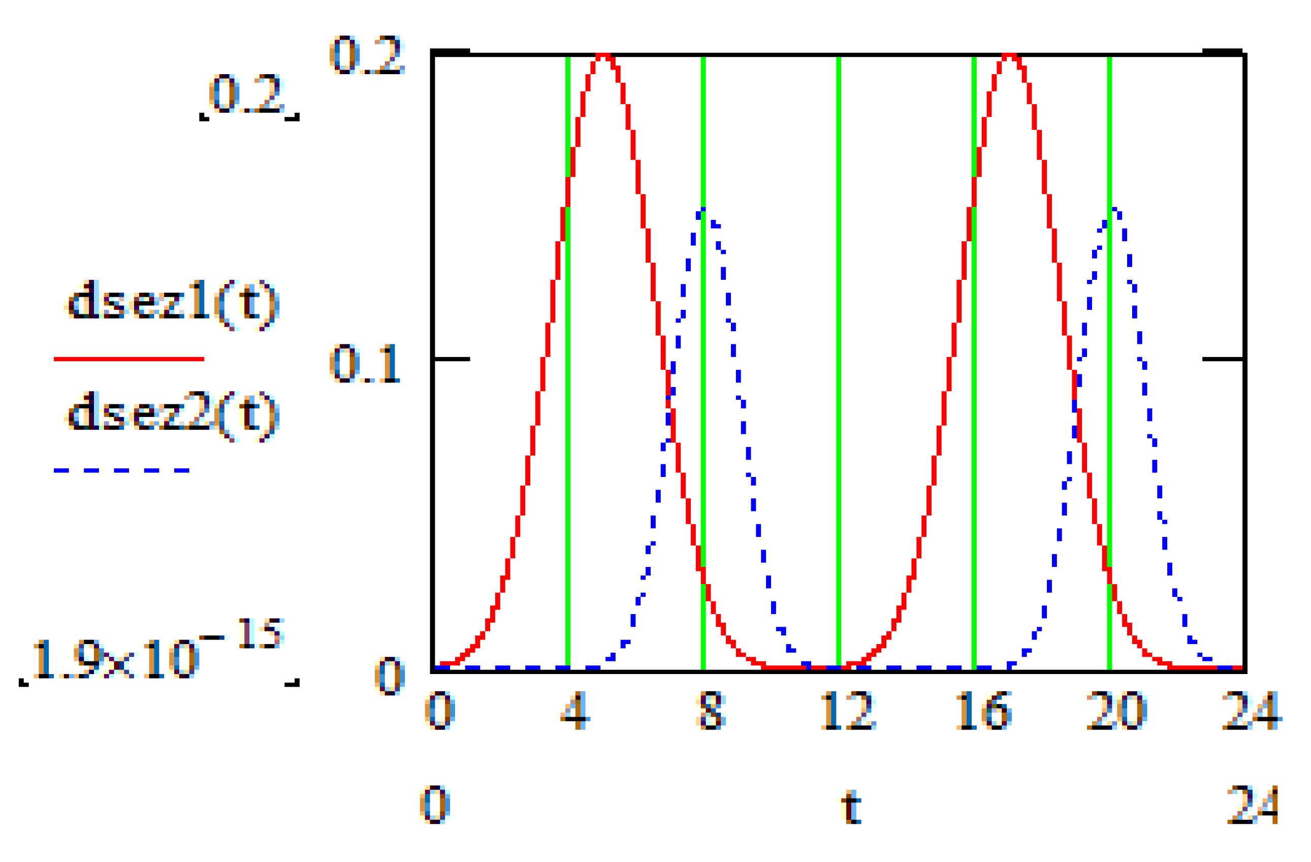
Let us consider the case of two seasonal upswings happening each month, ts1 and ts2, with the height, h1 and h2, related to D(t), and half-width, ϭ1 and ϭ2, respectively.

$$dsez1\left(t\right)=h1*e.$$

(12)

$$dsez2\left(t\right)=h2*\exp \left(-\frac{{\left(mod\left(t,12\right)-ts2\right)}^2}{2ϭ2^2}\right).$$

(13)

Seasonal demand fluctuations are graphically presented in Figure 1.

Using the above function, we define overall relative seasonal demand deviation in month t from the guaranteed amount as:

$$ds1\left(t,ks\right)=ks·As\left(t\right),$$

(14)

where ks is a seasonal deviation factor; at ks = 0, the seasonal deviations are not taken into account.

$$As\left(t\right)=dsez1\left(t\right)+dsez2\left(t\right)-{\displaystyle \sum }_{k=1}^{12}(dsez1\left(k\right)+dsez2\left(k\right))/12;$$

(15)

We assume that the seasonal demand fluctuations do not change the guaranteed amount of demand:

$${{\displaystyle \sum }}_{\mathrm{t}=t0}^{\mathrm{t}0+11}ds1\left(t,ks\right)=0.$$

The market demand for production of the sales enterprise, considering the seasonal fluctuations, is as follows:

$$Ds\left(t,ks\right)=D\left(t\right)·\left(1+ds1\left(t,ks\right)\right)=D\left(t\right)·\left(1+ks·As\left(t\right)\right).$$

(16)

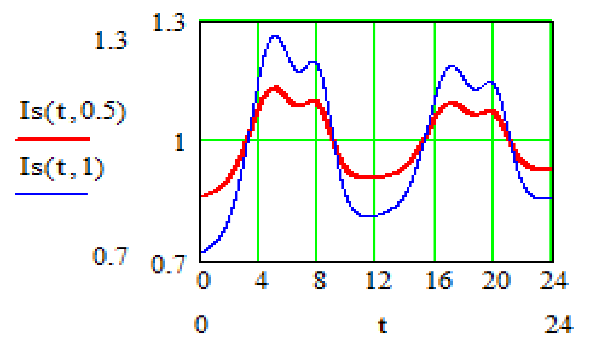
Let us define the month seasonal demand fluctuations index:

$$Is\left(t,rs\right)=\frac{Ds\left(t,ks\right)}{D\left(t\right)}=1+ks·As\left(t\right).$$

(17)

The expression reflects interrelation between the value of coefficient ks and index of the monthly demand fluctuations. By structure, the function $As\left(t\right)$has local maximums in months ts1, ts2 (Figure 2).

3.2.2. Random Demand Fluctuations

The market demand depends on real conditions, not only on seasonal fluctuations, but also on different social and economic factors [25,26] that cannot be unambiguously forecasted and defined with an explicit formula. We will take into consideration influence of such factors by introducing into the system a time-dependent random function (random process [36]) which we assume to be normally distributed [37].

Herewith, we assume the mathematical expectation and mean-square deviation to be equal to the function Ds (t, ks) and the value of σD(t) respectively, where σ is a scale parameter (for example, σ = 0.2). To build a function with such properties, we generate N normally distributed random sampling numbers, ${ƹ}_{t },t=1\dots N$, with mean-square deviation σ·D(t) (N: period of time in months, for which calculations of the system dynamics are performed; for example, N = 60). We obtain normally distributed variable ${ƹ}_{t }\sigma$ and write down the random demand fluctuation in month t as:

$$Dr\left(kr,t\right)=D\left(t\right)\ast ds2\left(kr,t\right),$$

(18)

$$\mathrm{here}ds2\left(kr,t\right)={ƹ}_{t }·\sigma ·kr$$

(19)

–the absolute and the relative random fluctuations of the demand in month t respectively.

kr: coefficient taking into account random deviations of demand; at kr = 0 the fluctuations are omitted.

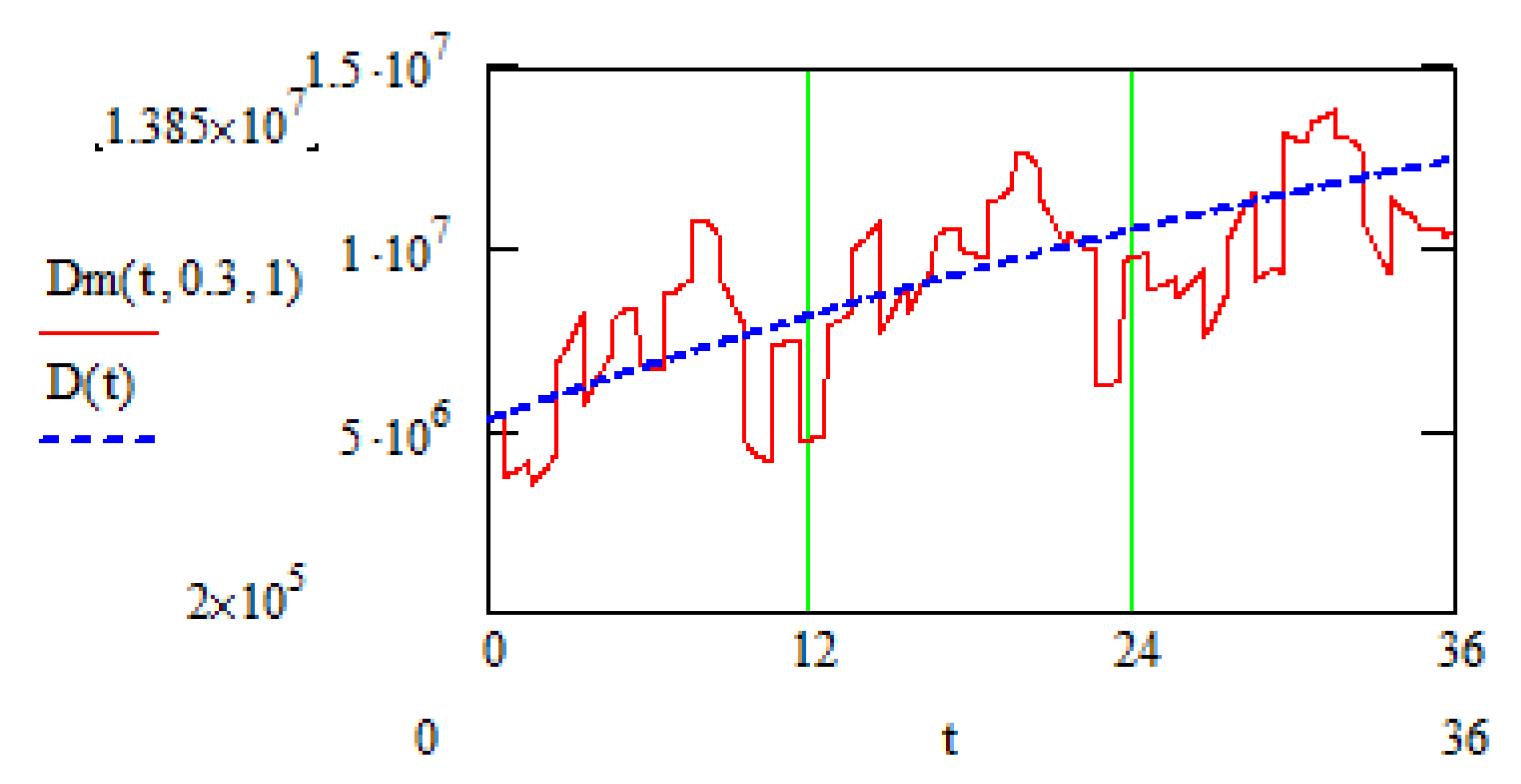
Total demand fluctuation amount is a sum of two components:

$$Dm\left(t,kr,ks\right)=Dr\left(kr,t\right)+Dsum\left(t,ks\right)$$

(20)

or

$$Dm\left(t,kr,ks\right)=D\left(t\right)\left(1+kr·{ƹ}_{t }·\sigma +ks·As\left(t\right)\right).$$

(21)

Function $Dm\left(t,kr,ks\right)$ describes the value of market demand for the investigated enterprises’ products in month t considering both seasonal and random fluctuations. (Figure 3).

3.3. Numeric Calculations

3.3.1. Influence of Seasonal Demand Fluctuations on the System Dynamics

We have performed investigation of the demand seasonal fluctuations impact on the main economic parameters using the above adduced calculation scheme. In the present model, the time variable is discrete and changes with a step of 1 month in accordance with the considered planning and reporting system. Dynamics calculations based on the recurrent equations allowed us to investigate both the influence of separate factors and their total impact on the system evolution.

Relative divergence of consumer demand from the guaranteed level, D(t), in month t is set in Formula (16) by a coefficient ks. It has been defined that in the months, when due to the seasonal fluctuations of the market deviation of the demand level is positive, the function Is(t,rs) is an increasing function of the value ks; with the increase of the coefficient ks from 0 to 1, the index of demand Is(t) grows from 0.9 to 1.5; while in the months of the negative demand deviation, it falls within the same interval. For analyzing the influence of seasonal fluctuations solely, we set $kr=0 \mathrm{and} ks>0.$

Value of the factors defining main conditions of the group activity, such as the level of labor cost, product prices at the markets, size of the investments, labor productivity, are different for the enterprises within the association. Actually, the production enterprises function in different conditions, and this is reflected in the dynamics of their economic parameters. The level of investments and size of orders were defined as the key factors. Due to the comparatively low price of labor in Ukraine, the enterprise Mriya has comparative advantages against the enterprise Emitex. However, bigger production capacities may compensate these advantages. As a result, an equilibrium state is set, in which changes in exogenous parameters like consumer demand fluctuations may qualitatively influence the economic dynamics.

A factor that helps to balance positions of the production enterprises is the synergetic principle lying in the basis of allocating reinvested capital, as described by Formulas (4)–(8). The share of investments to be allocated is defined depending on efficiency of each enterprise, and the less successful enterprise obtains an additional part of the investments at the expense of the more effective one. This circumstance is a partly compensating influence of the potentially unfavorable exogenous conditions, of which solely the demand/orders fluctuations are taken into account here.

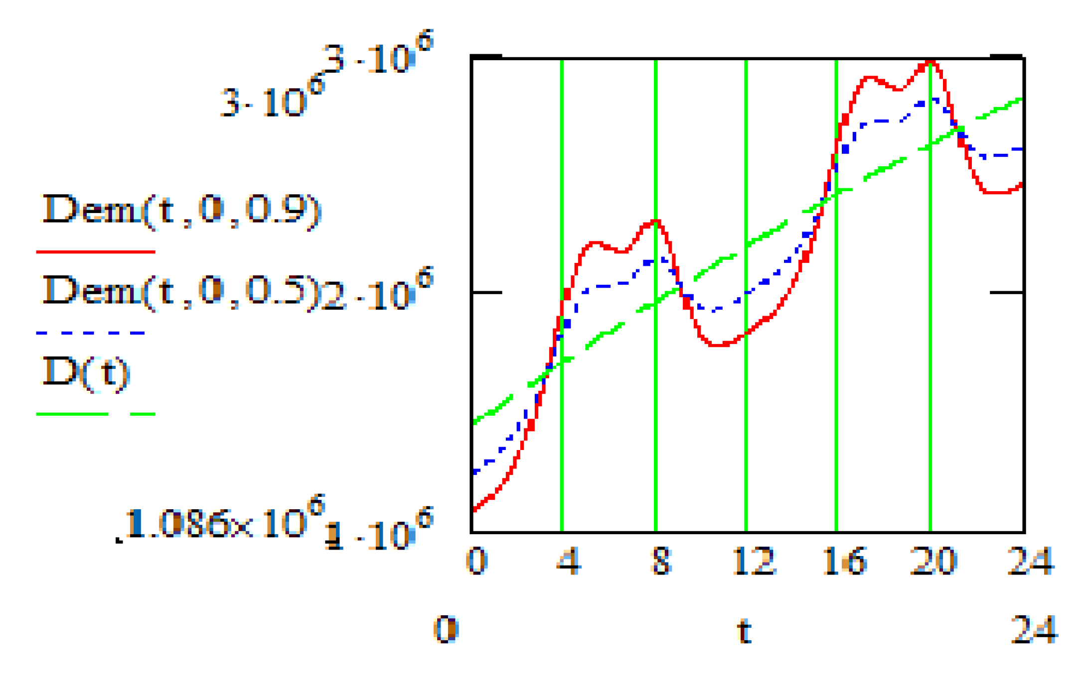
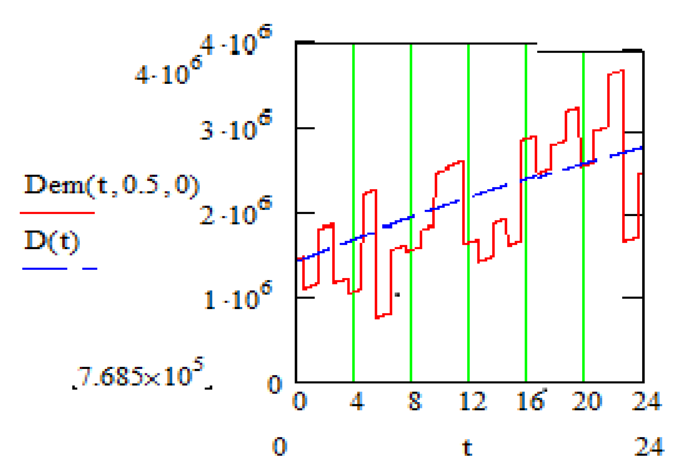
On Figure 4, the demand fluctuations considered in further calculations are presented at different levels of the coefficient ks, showing relative deviation from the guaranteed demand. Random factors/fluctuations are not considered here: kr = 0.

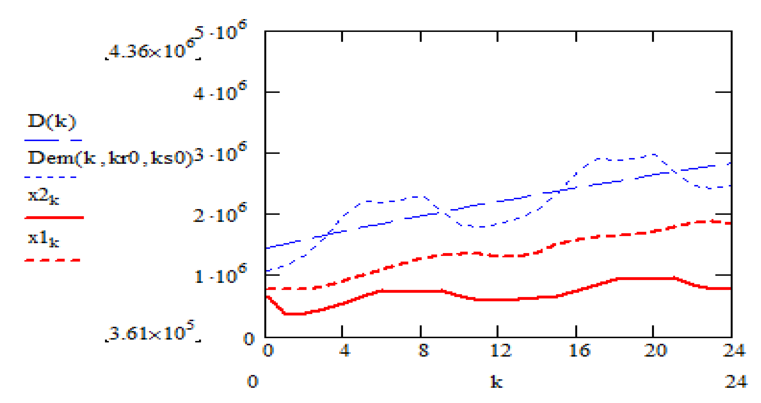
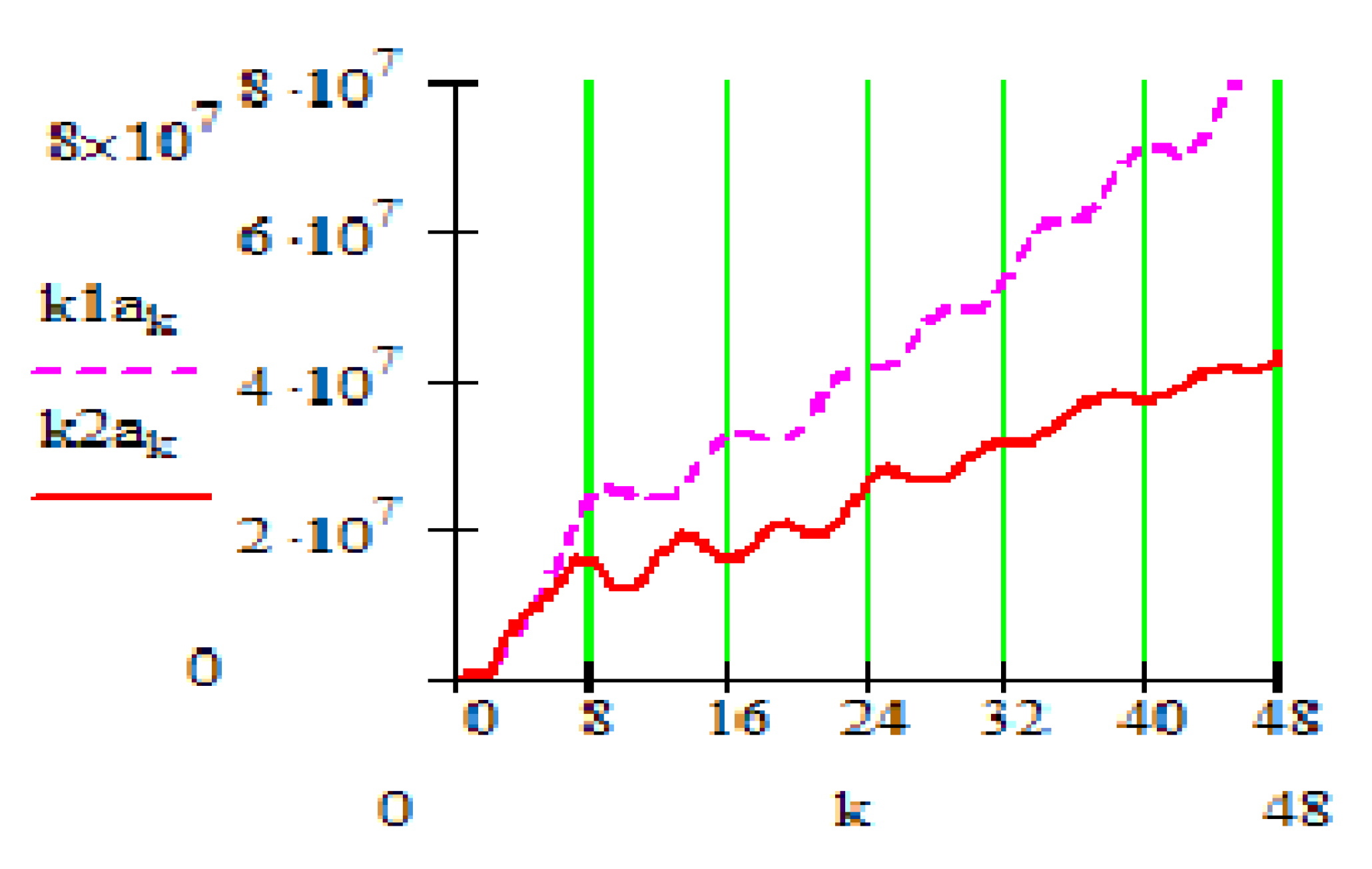
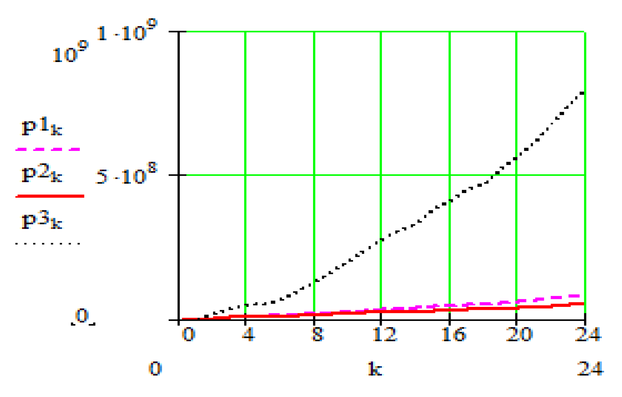
On Figure 5, Figure 6 and Figure 7 the impact of seasonal demand fluctuations on the level of invested capital, total capital and order size are presented.

The results of our calculations presented above prove that seasonal demand fluctuations provide for sizeable deviations in the total order size for the production companies, as well as changes in the level of reinvested capital. Relative deviations in the production level of the Polish company are bigger compared to the Ukrainian company, which fits into the implemented structure of orders allocation within the group. Herein, the relative changes in their own production companies’ capital are less sizeable.

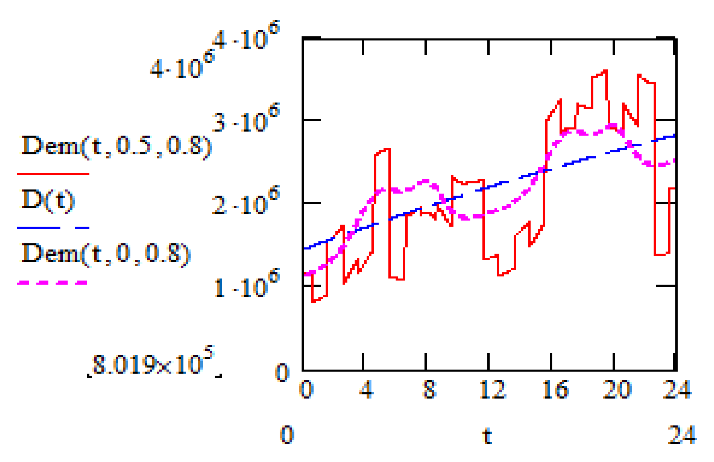
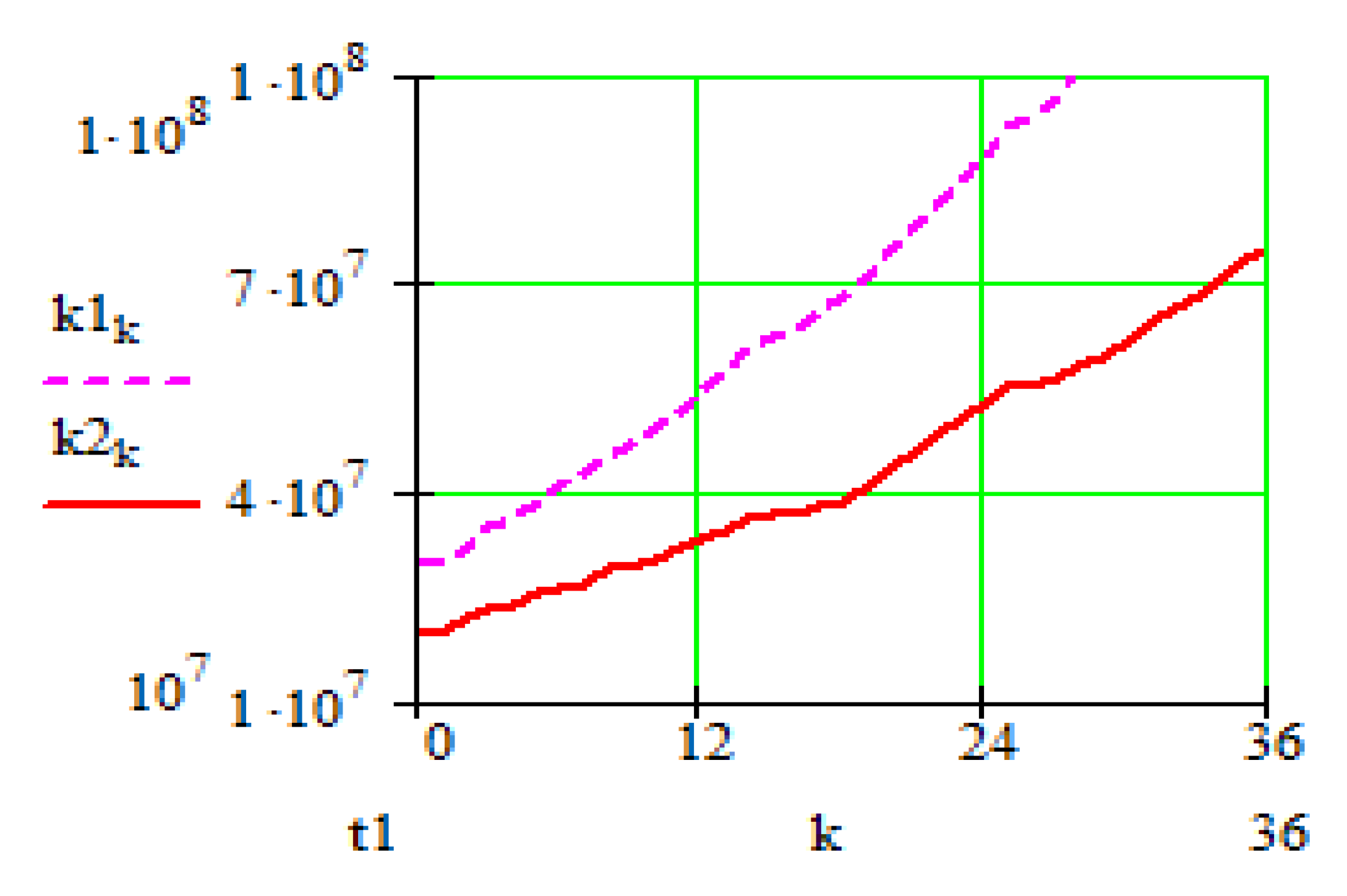
3.3.2. Total Impact of the Seasonal and Random Fluctuations on the System Dynamics

Further, we presented the results of calculations, considering also the random fluctuations. In the calculations, we set the values of coefficients that take into account seasonal and random fluctuations, ks = 0.8 and kr = 0.5, respectively. Graphs that reflect demand fluctuations are presented on Figure 8 and Figure 9.

Monthly changes in the level of profit, capital and investments are presented on the Figure 10, Figure 11 and Figure 12 below.

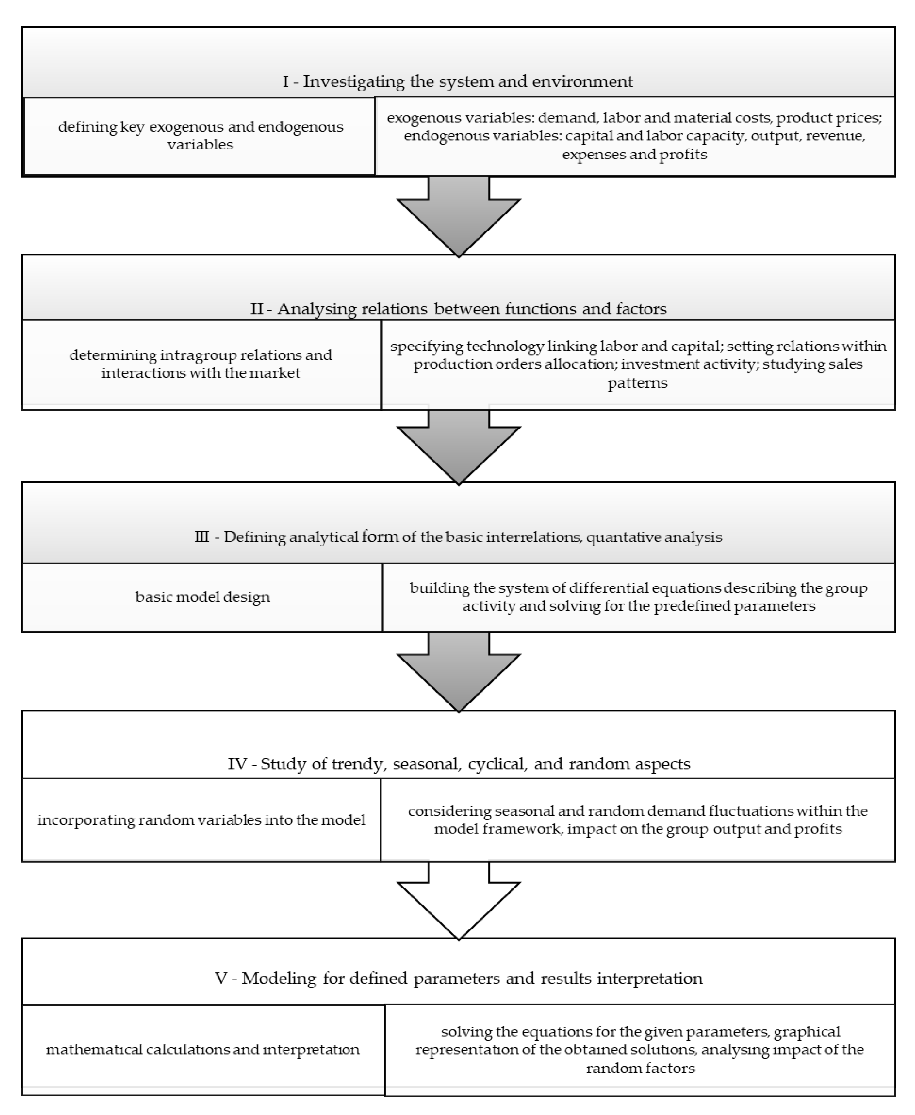
The main steps undertaken within the model described may be summarized in a flowchart presented further (Figure 13); the steps I-III were covered in more detail in the previous publications, while steps IV-V are described merely in the presented work.

4. Conclusions

Calculations of the economic dynamics according to a mathematical model create unique conditions for investigating economic systems. An adequate economic model allows investigation of both distinct influence of different factors, and joint influence of a number of factors in different combinations. Existing software provide for little time consumption needed for such investigations. At the same time, an imitational model provides a base for obtaining information on characteristics of the analyzed economic unit without intruding into its activity. A possibility arises for experiments with certain objects or groups of objects without any financial or social risks, as well as for obtaining information while avoiding lengthy statistics processing and dependence on the data availability concerning some external social or climate conditions.

Forecasting economic unit evolution within the framework of certain social-economic environments is necessary for elaborating appropriate financial and managerial strategy.

The suggested methodology, considering the impact of the changes in order level within the group of production and sales companies, allows the development of forecasts regarding evolution of its economic indexes. The given methodology allows analysis of the separate or combined influence of seasonal and random demand fluctuations on the main economic indexes of the companies. The possibility of investigating endogenous parameters variations within the model framework provides for a big scope of potential research. In particular, the presented results prove that seasonal demand fluctuations, which do not change the total amount of average annual demand and only re-locate it by periods during a year, do not have significant influence on the activity of production enterprises given sufficient production capacities. Demand fluctuations impact is typically more significant for a production company with weaker position, compared to similar companies. The reasons could lie in smaller production capacities, higher variable labor costs, high fixed costs, etc. Investigating the impact of such reasons in combination with other relevant factors, in particular with the help of suggested methodology, may be meaningful.

Possible further applications of the presented modeling approach include investigating the impact of other random external factors on the activity of companies, say, shocks in the political and social environment impacting the level of interest rates and considering such shocks in financial forecasting and Net Present Value (NPV) analysis of different projects. The method presented in the article concerns random variables affecting demand in each period of the group activity (monthly), while analyzing the variables with different behavior, say, undergoing some more rare random alterations (i.e., once or twice a year) are also of interest for further research; such variables may comprise effects on demand caused by unpredictable seasonal illnesses or pandemics.