The Global Well-Posedness for Large Amplitude Smooth Solutions for 3D Incompressible Navier–Stokes and Euler Equations Based on a Class of Variant Spherical Coordinates

Abstract

This paper investigates the globally dynamical stabilizing effects of the geometry of the domain at which the flow locates and of the geometry structure of the solutions with the finite energy to the three-dimensional (3D) incompressible Navier–Stokes (NS) and Euler systems. The global well-posedness for large amplitude smooth solutions to the Cauchy problem for 3D incompressible NS and Euler equations based on a class of variant spherical coordinates is obtained, where smooth initial data is not axi-symmetric with respect to any coordinate axis in Cartesian coordinate system. Furthermore, we establish the existence, uniqueness and exponentially decay rate in time of the global strong solution to the initial boundary value problem for 3D incompressible NS equations for a class of the smooth large initial data and a class of the special bounded domain described by variant spherical coordinates.

1. Introduction

In this paper, we consider the Cauchy problem for the three-dimensional (3D) incompressible Navier–Stokes ($\nu >0$) and Euler ($\nu =0$) equations

$$\begin{array}{c}\hfill \left\{\begin{array}{c}{\mathit{u}}_t+\mathit{u}·\nabla \mathit{u}+\nabla P=\nu \Delta \mathit{u},\mathit{x}\in {\mathbb{R}}^3,t>0,\hfill \\ \mathrm{div}\mathit{u}=0,\mathit{x}\in {\mathbb{R}}^3,t>0,\hfill \\ \mathit{u}(0,\mathit{x})={\mathit{u}}_0\left(\mathit{x}\right),\mathit{x}\in {\mathbb{R}}^3\hfill \end{array}\right.\end{array}$$

(1)

and the initial boundary value problem for the 3D incompressible Navier–Stokes ($\nu >0$) equations in the bounded domain

$$\begin{array}{c}\hfill \left\{\begin{array}{c}{\mathit{u}}_t+\mathit{u}·\nabla \mathit{u}+\nabla P=\nu \Delta \mathit{u},\mathit{x}\in \Omega ,t>0,\hfill \\ \mathrm{div}\mathit{u}=0,\mathit{x}\in \Omega ,t>0,\hfill \\ \mathit{u}=0,\mathit{x}\in \partial \Omega ,t>0,\hfill \\ \mathit{u}(0,\mathit{x})={\mathit{u}}_0\left(\mathit{x}\right),\mathit{x}\in \Omega \hfill \end{array}\right.\end{array}$$

(2)

respectively. Here, $\mathit{x}=(x_1,x_2,x_3)$, the unknown $\mathit{u}={(u^1(t,\mathit{x}),u^2(t,\mathit{x}),u^3(t,\mathit{x}))}^T$, denotes the fluid velocity vector field, $P=P(t,\mathit{x})$ is the scalar pressure, $\nu \ge 0$ is the viscosity coefficient. In addition, ${\mathit{u}}_0$ is a given initial velocity with $\mathrm{div}{\mathit{u}}_0=0$.

1.1. Background

It is well known that the 3D incompressible Navier–Stokes equations have at least one global weak solution with the finite energy [1,2]. However, the issue of the regularity and uniqueness for the global weak solution is still a challenging open problem in the field of mathematical fluid dynamics [3,4,5,6,7]. Furthermore, the 3D incompressible Euler equations have the unique smooth solution locally in time for any smooth initial data, but whether it is global in time is one open problem [5,8,9]. In particular, [9] describes some of the open problems related to the incompressible Euler equations, such as the blowup problem, the inviscid limit and anomalous dissipation.

Just because of this, many researchers are devoted to looking for certain sufficient conditions to ensure the smoothness of solutions, namely the regularity criterion or Serrin-type criterion. Thanks to the pioneering work by [7,10], we have known that the weak solution $\mathit{u}$ for the NS Equation (1) will be smooth as long as

$$\begin{array}{c}\mathit{u}\in L^p(0,T;L^q\left({\mathbb{R}}^3\right)),\frac{2}{p}+\frac{3}{q}\le 1,3\le q\le \infty .\hfill \end{array}$$

Afterwards, there are some progress on the regularity criteria involving only one component of the velocity fields, one can refer to [11,12,13,14,15] for details. Recently, [16] obtains a new regularity criterion which is weaker than every Ladyzhenskaya–Prodi–Serrin condition in the viscous case [7,10], and reduces to the Beale–Kato–Majda criterion in the inviscid case [8].

On the other hand, many researchers are concerned with the axisymmetric flow(one can see [5,15,17,18,19,20,21,22,23,24,25,26,27,28,29]), which makes the 3D flow close to 2D flow, that is, all velocity components (radial, angular (or swirl) and $x_3$-component) as well as the pressure are independent of the angular variable in the cylindrical coordinates. As a kind of fluid with special geometry structure, it is well known that the incompressible Navier–Stokes equations has a unique global regular solution, if the swirl component is zero, see [20,21,30,31]. However, it is still open for the global regularity with swirl, one can see [18,19] for related works.

Last year, [32,33] obtained new approach to solve the compressible Navier–Stokes equations in cylindrical coordinates. Motivated by this new approach and the helical flow (see [34] and references therein) of the 3D incompressible flows and on the absence of simple hyperbolic blow-up for the 3D incompressible Euler and quasi-geostrophic equations (see [35]), we investigate the globally dynamical stabilizing effects of the geometry of the domain at which the flow locates and of the geometry structure of the solutions to the three-dimensional incompressible flows by studying non-axisymmetric global smooth solution with respect to any coordinate axis $x_i,i=1,2,3$ in the Cartesian coordinate system in ${\mathbb{R}}^3$ and looking for the domain to guarantee the global wellposedness for the initial and boundary value problem for the 3D incompressible Navier–Stokes and Euler system based on a class of variant spherical coordinates.

It should be noted that we obtained a new class of large amplitude for the 3D incompressible NS and Euler equations based on variant spherical coordinates. The global smooth solutions are symmetric with respect to one straight line in ${\mathbb{R}}^3,$ not the Cartesian coordinate axis $x_i.$ Thus, our main results are complex and different from the classic $x_i$-axi-symmetric flow in cylindrical coordinates. Due to the different structures of the gradient, Laplacian and vorticity operators etc. in the different coordinate systems, the present results stated in Theorems 1–3 cannot be obtained directly from the global well-posedness results on classic axi-symmetric cylindrical coordinate flows.

These results lay a theoretical foundation of the numerical simulation for the 3D incompressible NS and Euler equations based on the variant spherical coordinates. In the future, we will study the well-posedness and numerical simulation of solutions for more similar models (such as 3D incompressible Boussinessq system and magnetohydrodynamic (MHD) system) based on the variant spherical coordinates.

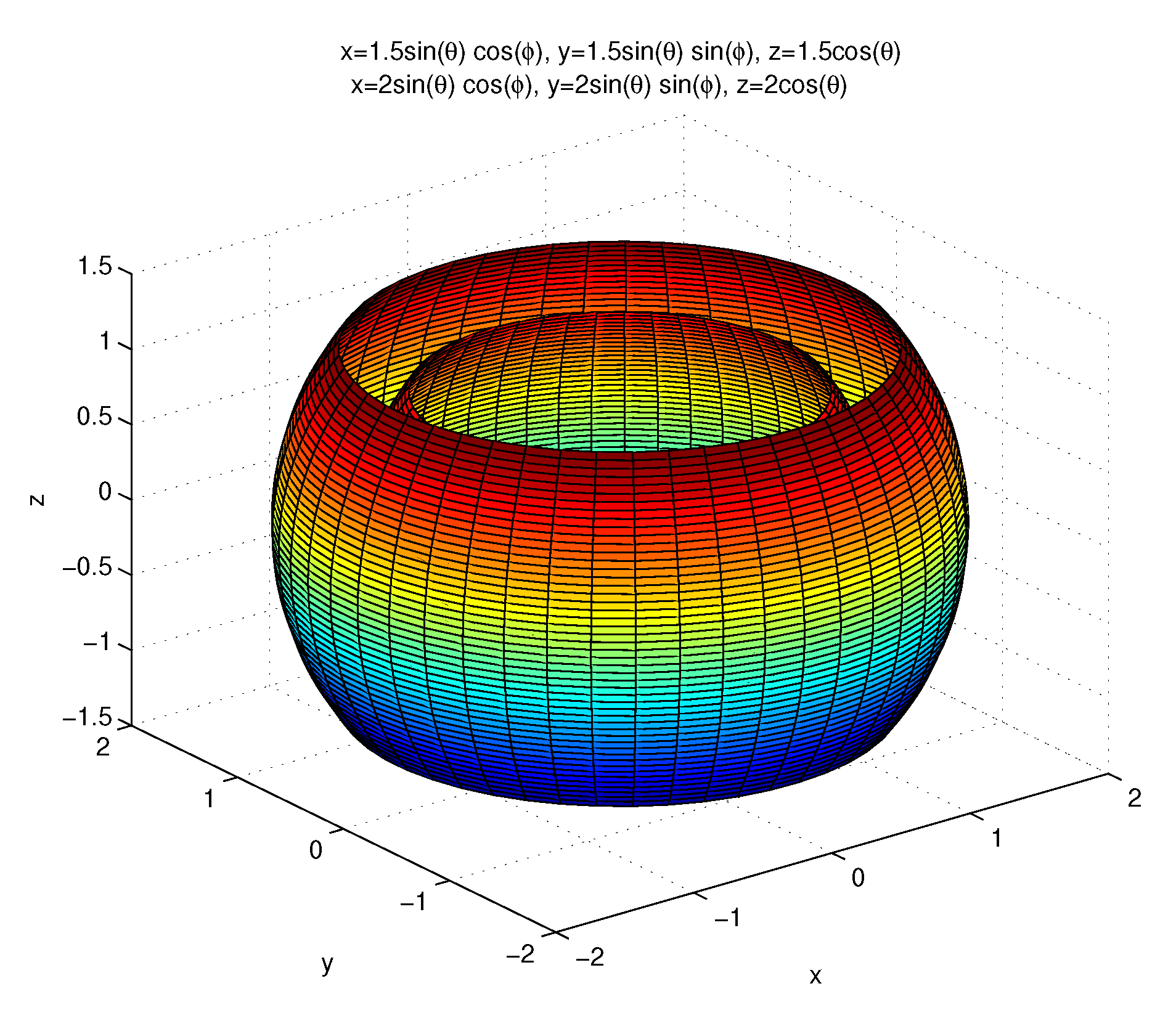
1.2. A Class of Variant Spherical Coordinates

Let the matrix

$$\mathit{A}=\left(\begin{array}{ccc}{a}_{11}& a_{12}& a_{13}\\ a_{21}& a_{22}& a_{23}\\ a_{31}& a_{32}& a_{33}\end{array}\right)$$

be a real orthogonal matrix, i.e., $A^{T}A=I$, where I is a identity matrix and $A^T$ is a transpose of the matrix A. For given $\mathit{\alpha }=\left(\begin{array}{c}{\alpha }_1\hfill \\ {\alpha }_2\hfill \\ {\alpha }_3\hfill \end{array}\right)\in {\mathbb{R}}^3$ and the constant $a>0$, introduce a class of variant spherical coordinates $(r,\theta ,\phi )$ defined as

$$\begin{array}{c}\hfill \mathit{x}=\left(\begin{array}{c}{x}_1\hfill \\ x_1\hfill \\ x_3\hfill \end{array}\right)=\left(\begin{array}{c}{\alpha }_1\hfill \\ {\alpha }_2\hfill \\ {\alpha }_3\hfill \end{array}\right)+a\mathit{A}\left(\begin{array}{c}rsin\theta cos\phi \\ rsin\theta sin\phi \\ rcos\theta \end{array}\right),\mathit{x}\in {\mathbb{R}}^3.\end{array}$$

(3)

Since the matrix A is an orthogonal one, we have

$$r=\frac{1}{a}\sqrt{{\xi }^2\left(\mathit{x}\right)+{\eta }^2\left(\mathit{x}\right)+{\zeta }^2\left(\mathit{x}\right)}=\frac{1}{a}\sqrt{{(x_1-{\alpha }_1)}^2+{(x_2-{\alpha }_2)}^2+{(x_3-{\alpha }_3)}^2}\ge 0,$$

$$0\le \theta =arctan\frac{\sqrt{{\xi }^2\left(\mathit{x}\right)+{\eta }^2\left(\mathit{x}\right)}}{\zeta \left(\mathit{x}\right)}\le \pi ,0\le \phi =arctan\frac{\eta \left(\mathit{x}\right)}{\xi \left(\mathit{x}\right)}<2\pi ,$$

where

$$\left\{\begin{array}{c}\xi \left(\mathit{x}\right)=a_{11}(x_1-{\alpha }_1)+a_{21}(x_2-{\alpha }_2)+a_{31}(x_3-{\alpha }_3),\hfill \\ \eta \left(\mathit{x}\right)=a_{12}(x_1-{\alpha }_1)+a_{22}(x_2-{\alpha }_2)+a_{32}(x_3-{\alpha }_3),\hfill \\ \zeta \left(\mathit{x}\right)=a_{13}(x_1-{\alpha }_1)+a_{23}(x_2-{\alpha }_2)+a_{33}(x_3-{\alpha }_3).\hfill \end{array}\right.$$

(4)

Note that, for variant spherical coordinates $(r,\theta ,\phi )$, r-coordinate is spherical symmetric in ${\mathbb{R}}^3$, but $\theta$-coordinate and $\phi$-coordinate are not axi-symmetric with respect to any coordinate axis $x_i,i=1,2,3$ in the Cartesian coordinate system $x\in {\mathbb{R}}^3$ except that $A=I$. Denote

$${\mathit{e}}_r=\mathit{A}\left(\begin{array}{c}sin\theta cos\phi \\ sin\theta sin\phi \\ cos\theta \end{array}\right)=\frac{1}{\sqrt{{\xi }^2\left(\mathit{x}\right)+{\eta }^2\left(\mathit{x}\right)+{\zeta }^2\left(\mathit{x}\right)}}\left(\begin{array}{c}{x}_1-{\alpha }_1\hfill \\ x_2-{\alpha }_2\hfill \\ x_3-{\alpha }_3\hfill \end{array}\right),$$

$${\mathit{e}}_{\theta }=\mathit{A}\left(\begin{array}{c}cos\theta cos\phi \\ cos\theta sin\phi \\ -sin\theta \end{array}\right)=\frac{\left(\begin{array}{c}{a}_{11}\xi \left(\mathit{x}\right)\zeta \left(\mathit{x}\right)+a_{12}\eta \left(\mathit{x}\right)\zeta \left(\mathit{x}\right)-a_{13}({\xi }^2\left(\mathit{x}\right)+{\eta }^2\left(\mathit{x}\right))\hfill \\ a_{21}\xi \left(\mathit{x}\right)\zeta \left(\mathit{x}\right)+a_{22}\eta \left(\mathit{x}\right)\zeta \left(\mathit{x}\right)-a_{23}({\xi }^2\left(\mathit{x}\right)+{\eta }^2\left(\mathit{x}\right))\hfill \\ a_{31}\xi \left(\mathit{x}\right)\zeta \left(\mathit{x}\right)+a_{32}\eta \left(\mathit{x}\right)\zeta \left(\mathit{x}\right)-a_{33}({\xi }^2\left(\mathit{x}\right)+{\eta }^2\left(\mathit{x}\right))\hfill \end{array}\right)}{\sqrt{{\xi }^2\left(\mathit{x}\right)+{\eta }^2\left(\mathit{x}\right)+{\zeta }^2\left(\mathit{x}\right)}\sqrt{{\xi }^2\left(\mathit{x}\right)+{\eta }^2\left(\mathit{x}\right)}},$$

$${\mathit{e}}_{\phi }=\mathit{A}\left(\begin{array}{c}-sin\phi \hfill \\ cos\phi \hfill \\ 0\hfill \end{array}\right)=\frac{1}{\sqrt{{\xi }^2\left(\mathit{x}\right)+{\eta }^2\left(\mathit{x}\right)}}\left(\begin{array}{c}-a_{11}\eta \left(\mathit{x}\right)+a_{12}\xi \left(\mathit{x}\right)\hfill \\ -a_{21}\eta \left(\mathit{x}\right)+a_{22}\xi \left(\mathit{x}\right)\hfill \\ -a_{31}\eta \left(\mathit{x}\right)+a_{32}\xi \left(\mathit{x}\right)\hfill \end{array}\right).$$

Furthermore, denote the special bounded domain $\tilde{\Omega }$ described by variant spherical coordinates by

$$\begin{array}{c}\tilde{\Omega }=\{(x_1,x_2,x_3)=({\alpha }_1+a{a}_{11}rsin\theta cos\phi +a{a}_{12}rsin\theta sin\phi +a{a}_{13}rcos\theta ,\hfill \\ {\alpha }_2+a{a}_{21}rsin\theta cos\phi +a{a}_{22}rsin\theta sin\phi +a{a}_{23}rcos\theta ,\hfill \\ {\alpha }_3+a{a}_{31}rsin\theta cos\phi +a{a}_{32}rsin\theta sin\phi +a{a}_{33}rcos\theta )\in {\mathbb{R}}^3:\hfill \\ 0<r_0\le r\le R_0<\infty ,0<{\theta }_0\le \theta \le {\theta }_1<\pi ,0\le \phi <2\pi \},\hfill \end{array}$$

(5)

where $r_0,R_0,{\theta }_0,{\theta }_1$ are given fixed positive constants. Here the domain $\tilde{\Omega }$ is non-smooth and symmetric on the straight line but non-$x_i$-axisymmetric for the Cartesian coordinates $x_1,x_2,x_3$ in ${\mathbb{R}}^3$. Moreover, the subset of the coordinate $x_i$ set in ${\mathbb{R}}^3$ can be included the inside of the domain $\tilde{\Omega }$. For example, $\tilde{\Omega }$ can be shown in Figure 1 by taking $a=1,A=I,r_0=1.5,R_0=2,{\theta }_0=0.3\pi ,{\theta }_1=0.7\pi$ and ${\alpha }_i(i=1,2,3)=0.$

Figure 1. The special bounded domain $\tilde{\Omega }$.

1.3. Research Model

Now we look for the solutions of the form

$$\mathit{u}(t,\mathit{x})=u^r(t,r,\theta ){\mathit{e}}_r+u^{\theta }(t,r,\theta ){\mathit{e}}_{\theta }+u^{\phi }(t,r,\theta ){\mathit{e}}_{\phi },P(t,\mathit{x})=P(t,r,\theta )$$

(6)

with

$${\mathit{u}}_0\left(\mathit{x}\right)=u_0^r(r,\theta ){\mathit{e}}_r+u_0^{\theta }(r,\theta ){\mathit{e}}_{\theta }+u_0^{\phi }(r,\theta ){\mathit{e}}_{\phi }$$

(7)

for the 3D incompressible Navier–Stokes and Euler Equations (1) and (2). Note that the solutions $(u^r,u^{\theta },u^{\phi })(t,r,\theta )$ given by (6) is not $x_i$-axisymmetric with respect to the Cartesian coordinates x because $\theta$-coordinate is non-axisymmetric with respect to the Cartesian coordinates $x\in {\mathbb{R}}^3$.

When the matrix A is an orthogonal matrix, the gradient operator ∇ and Laplacian $\Delta$ operator have the expression

$$\begin{array}{c}\nabla ={\mathit{e}}_r\frac{1}{a}{\partial }_r+\frac{1}{ar}{\mathit{e}}_{\theta }{\partial }_{\theta }+\frac{1}{arsin\theta }{\mathit{e}}_{\phi }{\partial }_{\phi }\hfill \end{array}$$

and

$$\begin{array}{c}\Delta =\frac{1}{a^2}({\partial }_r^2+\frac{2}{r}{\partial }_r+\frac{1}{r^2}{\partial }_{\theta }^2+\frac{cos\theta }{r^{2}sin\theta }{\partial }_{\theta }+\frac{1}{r^2{sin}^2\theta }{\partial }_{\phi }^2)\hfill \end{array}$$

respectively. Then one can derive the evolution equations for $(u^r,u^{\theta },u^{\phi })(r,\theta ,t)$ for 3D incompressible NS equations $\nu >0$ and for 3D incompressible Euler $\nu =0$ respectively as follows

$$\left\{\begin{array}{l}{\partial }_t{u}^r+(\tilde{\mathit{u}}·\tilde{\nabla })u^r+\frac{1}{a}{\partial }_{r}P=\nu [(\tilde{\Delta }-\frac{2}{a^2{r}^2})u^r-\frac{2cos\theta }{a^2{r}^{2}sin\theta }{u}^{\theta }-\frac{2}{a^2{r}^2}{\partial }_{\theta }{u}^{\theta }]+\frac{{(u^{\theta })}^2+{(u^{\phi })}^2}{ar},\\ {\partial }_t{u}^{\theta }+(\tilde{\mathit{u}}·\tilde{\nabla })u^{\theta }+\frac{1}{ar}{\partial }_{\theta }P=\nu [(\tilde{\Delta }-\frac{1}{a^2{r}^2{sin}^2\theta })u^{\theta }+\frac{2}{a^2{r}^2}{\partial }_{\theta }{u}^r]-\frac{u^r{u}^{\theta }}{ar}+\frac{cos\theta }{arsin\theta }{(u^{\phi })}^2,\\ {\partial }_t{u}^{\phi }+(\tilde{\mathit{u}}·\tilde{\nabla })u^{\phi }=\nu (\tilde{\Delta }-\frac{1}{a^2{r}^2{sin}^2\theta })u^{\phi }-\frac{u^r{u}^{\phi }}{ar}-\frac{cos\theta }{arsin\theta }{u}^{\theta }{u}^{\phi },\\ {\partial }_r{u}^r+\frac{2}{r}{u}^r+\frac{1}{r}{\partial }_{\theta }{u}^{\theta }+\frac{cos\theta }{rsin\theta }{u}^{\theta }=0\end{array}\right.$$

(8)

and

$$\left\{\begin{array}{l}{\partial }_t{u}^r+(\tilde{\mathit{u}}·\tilde{\nabla })u^r+\frac{1}{a}{\partial }_{r}P=\frac{{(u^{\theta })}^2+{(u^{\phi })}^2}{ar},\\ {\partial }_t{u}^{\theta }+(\tilde{\mathit{u}}·\tilde{\nabla })u^{\theta }+\frac{1}{ar}{\partial }_{\theta }P=-\frac{u^r{u}^{\theta }}{ar}+\frac{cos\theta }{arsin\theta }{(u^{\phi })}^2,\\ {\partial }_t{u}^{\phi }+(\tilde{\mathit{u}}·\tilde{\nabla })u^{\phi }=-\frac{u^r{u}^{\phi }}{ar}-\frac{cos\theta }{arsin\theta }{u}^{\theta }{u}^{\phi },\\ {\partial }_r{u}^r+\frac{2}{r}{u}^r+\frac{1}{r}{\partial }_{\theta }{u}^{\theta }+\frac{cos\theta }{rsin\theta }{u}^{\theta }=0\end{array}\right.$$

(9)

respectively, where $r\ge 0,0\le \theta \le \pi ,0\le \phi <2\pi ,t\ge 0$, $\tilde{\mathit{u}}=u^r{\mathit{e}}_r+u^{\theta }{\mathit{e}}_{\theta },$ and

$$\tilde{\nabla }={\mathit{e}}_r\frac{1}{a}{\partial }_r+{\mathit{e}}_{\theta }\frac{1}{ar}{\partial }_{\theta },\tilde{\Delta }=\frac{1}{a^2}({\partial }_r^2+\frac{2}{r}{\partial }_r+\frac{1}{r^2}{\partial }_{\theta }^2+\frac{cos\theta }{r^{2}sin\theta }{\partial }_{\theta }).$$

Note that Equations (8) and (9), called 3D incompressible NS and Euler equations in a class of variant spherical coordinates, completely determine the evolution of the 3D NS equations and 3D Euler equations a class of variant spherical coordinates respectively once the initial conditions and/or the boundary value conditions are given.

We take initial condition for the system (8) and (9) corresponding to the initial data (7) as follows:

$$(u^r,u^{\theta },u^{\phi })(t,r,\theta ){|}_{t=0}=(u_0^r,u_0^{\theta },u_0^{\phi })(r,\theta )$$

(10)

with given functions $u^r(r,\theta ),u^{\theta }(r,\theta )$ and $u^{\phi }(r,\theta )$.

Moreover, the boundary condition ${\mathit{u}|}_{\partial \Omega }=0,t\ge 0$ is equivalent to the following condition

$$(u^r,u^{\theta },u^{\phi }){|}_{\partial \Omega }=0,t\ge 0.$$

(11)

It is easy to know, by the direct computation, that the vorticity $\mathit{\omega }=\nabla \times \mathit{u}$ can be expressed as

$$\begin{array}{c}\mathit{\omega }(t,\mathit{x})={\omega }^r(t,r,\theta ){\mathit{e}}_r+{\omega }^{\theta }(t,r,\theta ){\mathit{e}}_{\theta }+{\omega }^{\phi }(t,r,\theta ){\mathit{e}}_{\phi }\hfill \end{array}$$

(12)

with the initial vorticity

$${\mathit{\omega }}_0=\mathit{\omega }(0,\mathit{x})={\omega }_0^r(r,\theta ){\mathit{e}}_r+{\omega }_0^{\theta }(r,\theta ){\mathit{e}}_{\theta }+{\omega }_0^{\phi }(r,\theta ){\mathit{e}}_{\phi },$$

(13)

where

$$\begin{array}{c}{\omega }^r=\frac{1}{arsin\theta }{\partial }_{\theta }(sin\theta u^{\phi }),{\omega }^{\theta }=-\frac{1}{ar}{\partial }_r(r{u}^{\phi }),{\omega }^{\phi }=\frac{1}{a}({\partial }_r{u}^{\theta }+\frac{u^{\theta }}{r}-\frac{{\partial }_{\theta }{u}^r}{r}).\hfill \end{array}$$

It is clear that

$$\begin{array}{c}\mathrm{div}\mathit{\omega }=\frac{1}{a}({\partial }_r{\omega }^r+\frac{2}{r}{\omega }^r+\frac{1}{r}{\partial }_{\theta }{\omega }^{\theta }+\frac{cos\theta }{rsin\theta }{\omega }^{\theta })\equiv 0.\hfill \end{array}$$

In addition, we can obtain the equation of ${\omega }_{\phi }$ from (8) as

$$\begin{array}{c}{\partial }_t{\omega }^{\phi }+(\tilde{\mathit{u}}·\tilde{\nabla }){\omega }^{\phi }=\nu (\tilde{\Delta }-\frac{1}{a^2{r}^2{sin}^2\theta }){\omega }^{\phi }+\frac{u^r{\omega }^{\phi }}{ar}+\frac{cos\theta }{arsin\theta }{u}^{\theta }{\omega }^{\phi }+(\frac{cos\theta }{arsin\theta }{\partial }_r-\frac{1}{a{r}^2}{\partial }_{\theta }){|u^{\phi }|}^2\hfill \end{array}$$

(14)

and from (9) as

$$\begin{array}{c}{\partial }_t{\omega }^{\phi }+(\tilde{\mathit{u}}·\tilde{\nabla }){\omega }^{\phi }=\frac{u^r{\omega }^{\phi }}{ar}+\frac{cos\theta }{arsin\theta }{u}^{\theta }{\omega }^{\phi }+(\frac{cos\theta }{arsin\theta }{\partial }_r-\frac{1}{a{r}^2}{\partial }_{\theta }){|u^{\phi }|}^2.\hfill \end{array}$$

(15)

1.4. Preliminaries

We provide some lemmas used for the proof of main theorems.

Lemma 1

(see [36]). Let $\mathit{u}\in W^{1,p}({\mathbb{R}}^3)$ is a velocity field with its divergence free and vorticity ω, then the inequality

$${\parallel \nabla \mathit{u}\parallel }_{L^p}\le C\left(p\right){\parallel \mathit{\omega }\parallel }_{L^p}$$

holds for any $p\in (1,\infty )$, where the constant $C\left(p\right)$ depends only on p.

Lemma 2

(see [30]). Let $D\subseteq {\mathbb{R}}^2,$ then there exists a constant $C\left(D\right)$ such that, for any $f\in H_0^1\left(D\right),$

$$\begin{array}{c}{∥f∥}_{L^4\left(D\right)}\le C\left(D\right){∥f∥}_{L^2\left(D\right)}^{\frac{1}{2}}{∥\nabla f∥}_{L^2\left(D\right)}^{\frac{1}{2}}.\hfill \end{array}$$

Lemma 3

(see [6,7,10]). Suppose that the initial data ${\mathit{u}}_0\in H^2({\mathbb{R}}^3)$ with $\mathrm{div}{\mathit{u}}_0=0$ in (1), then any Leray-Hopf weak solution $\mathit{u}$ of 3D incompressible Navier–Stokes Equation (1) is also a smooth solution in $(0,T]\times {\mathbb{R}}^3$ if there holds that

$$\mathit{u}\in L^p(0,T;L^q({\mathbb{R}}^3)),$$

in which p and q satisfy the conditions

$$\begin{array}{c}\frac{2}{p}+\frac{3}{q}\le 1with3<q<\infty ,2<p\le \infty orq=3,p=\infty .\hfill \end{array}$$

Lemma 4

(see [10,30]). Let $\Omega \subset {\mathbb{R}}^3$ be bounded and smooth. Suppose that the initial data ${\mathit{u}}_0\in H_0^1(\Omega )\cap H^2(\Omega )$ with $\mathrm{div}{\mathit{u}}_0=0$ in (2), then any Leray-Hopf weak solution to the initial boundary value problem (2) for 3D incompressible Navier–Stokes equations is also smooth in $(0,T]\times \Omega$ if the class of weak solution

$$\mathit{u}\in L^p(0,T;L^q(\Omega )),$$

in which p and q satisfy the conditions

$$\begin{array}{c}\frac{2}{p}+\frac{3}{q}\le 1with3<q\le \infty ,2\le p<\infty or3\le q<\infty ,p=\infty .\hfill \end{array}$$

Lemma 5

(see [5,8]). Let $\nu =0$ in (1) and $\mathit{u}$ be an unique smooth solution on interval $[0,T]$ to 3D incompressible Euler Equation (1) with $\nu =0$. Suppose that there are constants M and $T^{*}$ so that on any interval $[0,T]$ of existence of the solution $\mathit{u}$ with $T<T^{*},$ the vorticity satisfies the a priori estimate

$$\begin{array}{c}{\int }_0^{T^{*}}{\parallel \mathit{\omega }\parallel }_{L^{\infty }({\mathbb{R}}^3)}dt\le M.\hfill \end{array}$$

Then the solution $\mathit{u}$ can be continued to the interval$[0,T^{*}].$

2. Main Results

We now state our main results and prove them as follows:

Theorem 1.

(The global well-posedness for large amplitude smooth solutions to 3D Incompressible NS equations in ${\mathbb{R}}^3$ in the sense of variant spherical coordinates) Let $\nu >0$ in (8), $a>0,{\alpha }_i,i=1,2,3,$ be given constants, $A={(a_{ij})}_{i,j=1,2,3}$ be a real orthogonal matrix and the functions $\xi \left(\mathit{x}\right),\eta \left(\mathit{x}\right)$ and $\zeta \left({x}\right)$ be given by (4). Let ${\mathit{u}}_0\left(\mathit{x}\right)$ be given by

$$\begin{array}{ccc}\hfill {\mathit{u}}_0\left(\mathit{x}\right)& =& \frac{u_0^r(\frac{1}{a}\sqrt{{\xi }^2\left(\mathit{x}\right)+{\eta }^2\left(\mathit{x}\right)+{\zeta }^2\left(\mathit{x}\right)},arctan\frac{\sqrt{{\xi }^2\left(\mathit{x}\right)+{\eta }^2\left(\mathit{x}\right)}}{\zeta \left(\mathit{x}\right)})}{\sqrt{{\xi }^2\left(\mathit{x}\right)+{\eta }^2\left(\mathit{x}\right)+{\zeta }^2\left(\mathit{x}\right)}}\left(\begin{array}{c}{x}_1-{\alpha }_1\hfill \\ x_2-{\alpha }_2\hfill \\ x_3-{\alpha }_3\hfill \end{array}\right)\hfill \\ & +& \frac{u_0^{\theta }(\frac{1}{a}\sqrt{{\xi }^2\left(\mathit{x}\right)+{\eta }^2\left(\mathit{x}\right)+{\zeta }^2\left(\mathit{x}\right)},arctan\frac{\sqrt{{\xi }^2\left(\mathit{x}\right)+{\eta }^2\left(\mathit{x}\right)}}{\zeta \left(\mathit{x}\right)})}{\sqrt{{\xi }^2\left(\mathit{x}\right)+{\eta }^2\left(\mathit{x}\right)+{\zeta }^2\left(\mathit{x}\right)}\sqrt{{\xi }^2\left(\mathit{x}\right)+{\eta }^2\left(\mathit{x}\right)}}\hfill \\ & & \times \left(\begin{array}{c}{a}_{11}\xi \left(\mathit{x}\right)\zeta \left(\mathit{x}\right)+a_{12}\eta \left(\mathit{x}\right)\zeta \left(\mathit{x}\right)-a_{13}({\xi }^2\left(\mathit{x}\right)+{\eta }^2\left(\mathit{x}\right))\hfill \\ a_{21}\xi \left(\mathit{x}\right)\zeta \left(\mathit{x}\right)+a_{22}\eta \left(\mathit{x}\right)\zeta \left(\mathit{x}\right)-a_{23}({\xi }^2\left(\mathit{x}\right)+{\eta }^2\left(\mathit{x}\right))\hfill \\ a_{31}\xi \left(\mathit{x}\right)\zeta \left(\mathit{x}\right)+a_{32}\eta \left(\mathit{x}\right)\zeta \left(\mathit{x}\right)-a_{33}({\xi }^2\left(\mathit{x}\right)+{\eta }^2\left(\mathit{x}\right))\hfill \end{array}\right),\hfill \end{array}$$

(16)

where $u_0^r(r,\theta )$ and $u_0^{\theta }(r,\theta )$ are any given smooth functions. If ${\mathit{u}}_0(\mathit{x})\in H_0^1({\mathbb{R}}^3)\cap H^2({\mathbb{R}}^3)$ with $\mathrm{div}{\mathit{u}}_0=0$ and

$$\begin{array}{c}\hfill {\int }_{{\mathbb{R}}^3}{\left|\frac{\nabla \times {\mathit{u}}_0\left(\mathit{x}\right)}{\sqrt{{\xi }^2\left(\mathit{x}\right)+{\eta }^2\left(\mathit{x}\right)}}\right|}^{2}d\mathit{x}\le C<\infty ,\end{array}$$

(17)

then the Cauchy problem (1) with $\nu >0$ for 3D incompressible Navier–Stokes equations has a unique global strong solution $(\mathit{u},P)(t,\mathit{x})$ in time having the form

$$\begin{array}{ccc}\hfill \mathit{u}(t,\mathit{x})& =& \frac{u^r(t,\frac{1}{a}\sqrt{{\xi }^2\left(\mathit{x}\right)+{\eta }^2\left(\mathit{x}\right)+{\zeta }^2\left(\mathit{x}\right)},arctan\frac{\sqrt{{\xi }^2\left(\mathit{x}\right)+{\eta }^2\left(\mathit{x}\right)}}{\zeta \left(\mathit{x}\right)})}{\sqrt{{\xi }^2\left(\mathit{x}\right)+{\eta }^2\left(\mathit{x}\right)+{\zeta }^2\left(\mathit{x}\right)}}\left(\begin{array}{c}{x}_1-{\alpha }_1\hfill \\ x_2-{\alpha }_2\hfill \\ x_3-{\alpha }_3\hfill \end{array}\right)\hfill \\ & +& \frac{u^{\theta }(t,\frac{1}{a}\sqrt{{\xi }^2\left(\mathit{x}\right)+{\eta }^2\left(\mathit{x}\right)+{\zeta }^2\left(\mathit{x}\right)},arctan\frac{\sqrt{{\xi }^2\left(\mathit{x}\right)+{\eta }^2\left(\mathit{x}\right)}}{\zeta \left(\mathit{x}\right)})}{\sqrt{{\xi }^2\left(\mathit{x}\right)+{\eta }^2\left(\mathit{x}\right)+{\zeta }^2\left(\mathit{x}\right)}\sqrt{{\xi }^2\left(\mathit{x}\right)+{\eta }^2\left(\mathit{x}\right)}}\hfill \\ & & \times \left(\begin{array}{c}{a}_{11}\xi \left(\mathit{x}\right)\zeta \left(\mathit{x}\right)+a_{12}\eta \left(\mathit{x}\right)\zeta \left(\mathit{x}\right)-a_{13}({\xi }^2\left(\mathit{x}\right)+{\eta }^2\left(\mathit{x}\right))\hfill \\ a_{21}\xi \left(\mathit{x}\right)\zeta \left(\mathit{x}\right)+a_{22}\eta \left(\mathit{x}\right)\zeta \left(\mathit{x}\right)-a_{23}({\xi }^2\left(\mathit{x}\right)+{\eta }^2\left(\mathit{x}\right))\hfill \\ a_{31}\xi \left(\mathit{x}\right)\zeta \left(\mathit{x}\right)+a_{32}\eta \left(\mathit{x}\right)\zeta \left(\mathit{x}\right)-a_{33}({\xi }^2\left(\mathit{x}\right)+{\eta }^2\left(\mathit{x}\right))\hfill \end{array}\right),\hfill \end{array}$$

(18)

namely, the Cauchy problem (8) and (10) has a unique global strong solution $(u^r,u^{\theta },u^{\phi },P)(t,r,\theta )$ with $u^{\phi }\equiv 0$, and satisfying $u\in L^{\infty }(0,+\infty ;H^1({\mathbb{R}}^3))$.

Moreover, assume also that ${\mathit{u}}_0\left(\mathit{x}\right)$ is smooth, then the Cauchy problem (1) with $\nu >0$ for the 3D incompressible Navier–Stokes equations has a unique global smooth solution in time.

Proof of Theorem 1.

Noting that the unit vectors ${\mathit{e}}_r,{\mathit{e}}_{\theta },{\mathit{e}}_{\phi }$ are orthogonal because the matrix A is assumed to be one orthogonal matrix. Form (1) with $\nu >0$, for any $T>0,$ we have the energy inequality

$$\begin{array}{c}{\displaystyle \underset{0\le t\le T}{sup}}{∥\mathit{u}∥}_{L^2({\mathbb{R}}^3)}^2+2\nu {\int }_0^T{∥\nabla \mathit{u}∥}_{L^2({\mathbb{R}}^3)}^{2}dt\le {∥{\mathit{u}}_0∥}_{L^2({\mathbb{R}}^3)}^2.\hfill \end{array}$$

(19)

Under the assumptions of Theorem 1 on initial data, we have that $u_0^{\phi }\equiv 0,$ and, hence, $u^{\phi }(t,r,\theta )\equiv 0$ by local well-posedness theory. Thus, the velocity $\mathit{u}(t,\mathit{x})$ and vorticity $\mathit{\omega }(t,\mathit{x})=(\nabla \times \mathit{u})(t,x)$ satisfy the following special form

$$\mathit{u}(t,\mathit{x})=u^r(t,r,\theta ){\mathit{e}}_r+u^{\theta }(t,r,\theta ){\mathit{e}}_{\theta },\mathit{\omega }(t,\mathit{x})={\omega }^{\phi }(t,r,\theta ){\mathit{e}}_{\phi },$$

(20)

and, hence, the Equation (14) for ${\omega }^{\phi }$ is simplified as

$$\begin{array}{c}{\partial }_t{\omega }^{\phi }+(\tilde{\mathit{u}}·\tilde{\nabla }){\omega }^{\phi }=\nu (\tilde{\Delta }-\frac{1}{a^2{r}^2{sin}^2\theta }){\omega }^{\phi }+\frac{u^r{\omega }^{\phi }}{ar}+\frac{cos\theta }{arsin\theta }{u}^{\theta }{\omega }^{\phi }.\hfill \end{array}$$

(21)

By multiplying (21) by $r^2{sin}^2\theta$ and then letting $r=0$ or $\theta =0$ or $\theta =\pi$, it is easy to see that

$${\omega }^{\phi }(t,0,\theta )={\omega }^{\phi }(t,r,0)={\omega }^{\phi }(t,r,\pi )=0.$$

Putting

$${\omega }^{\phi }(t,r,\theta )=g(t,r,\theta )arsin\theta ,$$

i.e., $g(t,r,\theta )=\frac{{\omega }^{\phi }(t,r,\theta )}{arsin\theta }$ into (21), we obtain the following equation for $g(t,r,\theta )$

$$\begin{array}{c}{\partial }_{t}g+(\tilde{u}·\tilde{\nabla })g-\nu \tilde{\Delta }g=2\nu (\frac{1}{a^{2}r}{\partial }_r+\frac{cos\theta }{a^2{r}^{2}sin\theta }{\partial }_{\theta })g.\hfill \end{array}$$

(22)

Multiplying the Equation (22) by g and integrating the resulting equation on ${\mathbb{R}}^3$, we have

$$\begin{array}{l}\frac{1}{2}\frac{d}{dt}{∥g∥}_{L^2({\mathbb{R}}^3)}^2+\nu {\parallel \tilde{\nabla }g\parallel }_{L^2({\mathbb{R}}^3)}^2\hfill \\ =\nu ({\int }_{{\mathbb{R}}^3}\frac{1}{a^{2}r}{\partial }_r{\left|g\right|}^{2}d\mathit{x}+{\int }_{{\mathbb{R}}^3}\frac{cos\theta }{a^2{r}^{2}sin\theta }{\partial }_{\theta }{\left|g\right|}^{2}d\mathit{x})\hfill \\ =a\nu ({\int }_0^{2\pi }{\int }_0^{\pi }{\int }_0^{\infty }(\frac{1}{r}{\partial }_r{\left|g\right|}^2)r^{2}sin\theta drd\theta d\phi +{\int }_0^{2\pi }{\int }_0^{\pi }{\int }_0^{\infty }(\frac{cos\theta }{r^{2}sin\theta }{\partial }_{\theta }{\left|g\right|}^2)r^{2}sin\theta drd\theta d\phi )\hfill \\ =a\nu ({\int }_0^{2\pi }{\int }_0^{\pi }{\int }_0^{\infty }rsin\theta {\partial }_r{\left|g\right|}^{2}drd\theta d\phi +{\int }_0^{2\pi }{\int }_0^{\pi }{\int }_0^{\infty }cos\theta {\partial }_{\theta }{\left|g\right|}^{2}drd\theta d\phi )\hfill \\ =a\nu {\int }_0^{2\pi }{\int }_0^{\pi }(g^2(t,r,\theta )rsin\theta ){|}_{r=0}^{r=\infty }d\theta d\phi +a\nu {\int }_0^{2\pi }{\int }_0^{\infty }(g^2(t,r,\theta )cos\theta ){|}_{\theta =0}^{\theta =\pi }drd\phi \hfill \\ -a\nu ({\int }_0^{2\pi }{\int }_0^{\pi }{\int }_0^{\infty }{\left|g\right|}^{2}sin\theta ({\partial }_{r}r)drd\theta d\phi +{\int }_0^{2\pi }{\int }_0^{\pi }{\int }_0^{\infty }{\left|g\right|}^2{\partial }_{\theta }(cos\theta )drd\theta d\phi )\hfill \\ =-a\nu {\int }_0^{2\pi }{\int }_0^{\infty }(g^2(t,r,0)+g^2(t,r,\pi ))drd\phi -0\hfill \\ \le 0,\hfill \end{array}$$

which yields to the following estimate for $g(t,r,\theta )$

$$\begin{array}{c}{\parallel g(t,r,\theta )\parallel }_{L^2({\mathbb{R}}^3)}\le {\parallel g(0,r,\theta )\parallel }_{L^2({\mathbb{R}}^3)}=\parallel \frac{{\omega }_0^{\phi }(r,\theta )}{arsin\theta }{\parallel }_{L^2({\mathbb{R}}^3)}=\parallel \frac{(\nabla \times {\mathit{u}}_0)\left(\mathit{x}\right)}{\sqrt{{\xi }^2\left(\mathit{x}\right)+{\eta }^2\left(\mathit{x}\right)}}{\parallel }_{L^2({\mathbb{R}}^3)}\le C<\infty \hfill \end{array}$$

(23)

by using assumption (17) in Theorem 1, the fact that $|{\mathit{e}}_{\phi }|=1$ and the transform (3).

Next, we obtain the estimate for the vorticity $\omega ={\omega }^{\phi }(t,r,\theta ){\mathit{e}}_{\phi }$, given by (20) in the case of no swirl for 3D incompressible Navier–Stokes equation in a class of variant spherical coordinates.

It is known that the vorticity equation for the vorticity $\mathit{\omega }=\nabla \times \mathit{u}$ for 3D incompressible NS Equation is the following

$${\partial }_t\mathit{\omega }+(\mathit{u}·\nabla )\mathit{\omega }-\nu \Delta \mathit{\omega }=\mathit{\omega }·\nabla \mathit{u}.$$

(24)

Multiplying the Equation (24) by $\omega$ and integrating the resulting equation on ${\mathbb{R}}^3$, by using and (20), with the help of Hölder inequality, Gagliardo–Nirenberg inequality and Young inequality, we have, for any $T>0$, $0\le t\le T$,

$$\begin{array}{cc}& \frac{1}{2}\frac{d}{dt}{∥\mathit{\omega }∥}_{L^2\left({\mathbb{R}}^3\right)}^2+\nu {∥\nabla \mathit{\omega }∥}_{L^2\left({\mathbb{R}}^3\right)}^2\hfill \\ =& {\int }_{{\mathbb{R}}^3}(\mathit{\omega }·\nabla )\mathit{u}·\mathit{\omega }d\mathit{x}\hfill \\ =& {\int }_{{\mathbb{R}}^3}[{\omega }^{\phi }{\mathit{e}}_{\phi }·\frac{1}{a}({\mathit{e}}_r{\partial }_r+{\mathit{e}}_{\theta }\frac{1}{r}{\partial }_{\theta }+{\mathit{e}}_{\phi }\frac{1}{rsin\theta }{\partial }_{\phi })](u^r{\mathit{e}}_r+u^{\theta }{\mathit{e}}_{\theta })·\left({\omega }^{\phi }{\mathit{e}}_{\phi }\right)d\mathit{x}\hfill \\ =& {\int }_{{\mathbb{R}}^3}[\frac{{\omega }^{\phi }}{arsin\theta }{\partial }_{\phi }(u^r{\mathit{e}}_r+u^{\theta }{\mathit{e}}_{\theta })]·\left({\omega }^{\phi }{\mathit{e}}_{\phi }\right)d\mathit{x}\hfill \\ =& {\int }_{{\mathbb{R}}^3}[\frac{{\omega }^{\phi }}{arsin\theta }(u^{r}sin\theta +u^{\theta }cos\theta ){\mathit{e}}_{\phi }]·\left({\omega }^{\phi }{\mathit{e}}_{\phi }\right)d\mathit{x}\hfill \\ =& {\int }_{{\mathbb{R}}^3}\frac{1}{ar}{u}^r{\omega }^{\phi }{\omega }^{\phi }d\mathit{x}+{\int }_{{\mathbb{R}}^3}\frac{cos\theta }{arsin\theta }{u}^{\theta }{\omega }^{\phi }{\omega }^{\phi }d\mathit{x}\hfill \\ =& {\int }_{{\mathbb{R}}^3}{u}^{r}g{\omega }^{\phi }sin\theta d\mathit{x}+{\int }_{{\mathbb{R}}^3}{u}^{\theta }g{\omega }^{\phi }cos\theta d\mathit{x}\hfill \\ \le & {\int }_{{\mathbb{R}}^3}|u^{r}g{\omega }^{\phi }|d\mathit{x}+{\int }_{{\mathbb{R}}^3}|u^{\theta }g{\omega }^{\phi }|d\mathit{x}\hfill \\ \le & (\parallel u^r{\parallel }_{L^3\left({\mathbb{R}}^3\right)}+\parallel u^{\theta }{\parallel }_{L^3\left({\mathbb{R}}^3\right)}{)\parallel g\parallel }_{L^2\left({\mathbb{R}}^3\right)}{\parallel \mathit{\omega }\parallel }_{L^6\left({\mathbb{R}}^3\right)}\hfill \\ \le & C{∥\mathit{u}∥}_{L^2\left({\mathbb{R}}^3\right)}^{\frac{1}{2}}{∥\nabla \mathit{u}∥}_{L^2\left({\mathbb{R}}^3\right)}^{\frac{1}{2}}{∥g∥}_{L^2\left({\mathbb{R}}^3\right)}{∥\nabla \mathit{\omega }∥}_{L^2\left({\mathbb{R}}^3\right)}\hfill \\ \le & C{∥\mathit{u}∥}_{H^1\left({\mathbb{R}}^3\right)}^2+\frac{\nu }{2}{∥\nabla \mathit{\omega }∥}_{L^2\left({\mathbb{R}}^3\right)}^2,\hfill \end{array}$$

which, by applying the Gronwall’s inequality and by using (19), yields to, for any $T>0$,

$$\begin{array}{c}{\parallel \mathit{\omega }(t,·)\parallel }_{L^2\left({\mathbb{R}}^3\right)}\le C(T,\parallel {\mathit{u}}_0{\parallel }_{H^1\left({\mathbb{R}}^3\right)},\parallel \frac{(\nabla \times {\mathit{u}}_0)\left(\mathit{x}\right)}{\sqrt{{\xi }^2\left(\mathit{x}\right)+{\eta }^2\left(\mathit{x}\right)}}{\parallel }_{L^2\left({\mathbb{R}}^3\right)}),0\le t\le T,\hfill \\ {\int }_0^t{\parallel \nabla \mathit{\omega }(s,·)\parallel }_{L^2\left({\mathbb{R}}^3\right)}^{2}ds\le C(T,\parallel {\mathit{u}}_0{\parallel }_{H^1\left({\mathbb{R}}^3\right)},\parallel \frac{(\nabla \times {\mathit{u}}_0)\left(\mathit{x}\right)}{\sqrt{{\xi }^2\left(\mathit{x}\right)+{\eta }^2\left(\mathit{x}\right)}}{\parallel }_{L^2\left({\mathbb{R}}^3\right)}),0\le t\le T.\hfill \end{array}$$

(25)

Using Lemma 1, we get from (25) that, for any $0\le T\le \infty$,

$$\nabla \mathit{u}\in L^{\infty }(0,T;L^2\left({\mathbb{R}}^3\right)),$$

and, hence, by Sobolev’s imbedding Theorem, we have, for any $0\le T\le \infty$,

$$\mathit{u}\in L^{\infty }(0,T;L^6\left({\mathbb{R}}^3\right)).$$

Now the desired regularity estimate for 3D incompressible Navier–Stokes Equation (1) is obtained, hence, by applying Lemma 3, we obtain the results stated in Theorem 1.

The proof of Theorem 1 is complete. □

Theorem 2.

(The global well-posedness for large amplitude smooth solutions to 3D Incompressible Euler equations in ${\mathbb{R}}^3$ in the sense of variant spherical coordinates) Let $\nu =0$ in (1). Let ${\mathit{u}}_0\left(\mathit{x}\right)$ given by (16) be smooth with $\mathrm{div}{\mathit{u}}_0=0$. Let the assumptions in Theorem 1 holds. Furthermore, assume that

$$\begin{array}{c}\hfill {\int }_{{\mathbb{R}}^3}{\left|((\nabla \times {\mathit{u}}^0)\left(\mathit{x}\right),\frac{(\nabla \times {\mathit{u}}^0)\left(\mathit{x}\right)}{\sqrt{{\xi }^2\left(\mathit{x}\right)+{\eta }^2\left(\mathit{x}\right)}})\right|}^{p}d\mathit{x}\le C<\infty ,1\le p\le \infty .\end{array}$$

(26)

Then the Cauchy problem (1) with $\nu =0$ for 3D incompressible Euler equations has a unique global smooth solution $(\mathit{u},P)(t,\mathit{x})$ in time having the form (18), namely, the Cauchy problem (9) and (10) has a unique global smooth solution in time $(u^r,u^{\theta },u^{\phi },P)(t,r,\theta )$ with $u^{\phi }\equiv 0$, satisfying $\mathit{u}\in C^1([0,\infty ),H^s\left({\mathbb{R}}^3\right))$ with $s\ge \frac{5}{2}$.

Proof of Theorem 2.

We establish the global smooth solution in time for 3D incompressible Euler Equation (1) with $\nu =0$. The local well-posedness result for the smooth solution to the Cauchy problem for the 3D incompressible Euler equations, see [5]. By the existence and uniqueness of the local smooth solution to the Chauchy problem on 3D incompressible Euler equation, it is easy to obtain that $u^{\phi }(t,r,\theta )=0$ for all time because of the assumption that $u_0^{\phi }(r,\theta )=0$ on the initial data.

Firstly, we have the basic energy estimate from the local smooth solution to (1) with $\nu =0$

$$\begin{array}{c}\hfill {\parallel \mathit{u}(t,·)\parallel }_{L^2\left({\mathbb{R}}^3\right)}={\parallel {\mathit{u}}_0(·)\parallel }_{L^2\left({\mathbb{R}}^3\right)}.\end{array}$$

(27)

Because $u^{\phi }\equiv 0,$ the velocity and vorticity become the following special form (20) as in the case of Navier–Stokes equation

$$\mathit{u}(t,\mathit{x})=u^r(t,r,\theta ){\mathit{e}}_r+u^{\theta }(t,r,\theta ){\mathit{e}}_{\theta },\mathit{\omega }(t,\mathit{x})={\omega }^{\phi }(t,r,\theta ){\mathit{e}}_{\phi },$$

and the Equation (15) for ${\omega }^{\phi }$ becomes the following one

$$\begin{array}{c}{\partial }_t{\omega }^{\phi }+(\tilde{\mathit{u}}·\tilde{\nabla }){\omega }^{\phi }=\frac{u^r{\omega }^{\phi }}{ar}+\frac{cos\theta }{arsin\theta }{u}^{\theta }{\omega }^{\phi }.\hfill \end{array}$$

(28)

Denote $h(t,r,\theta )=\frac{{\omega }^{\phi }}{arsin\theta }$, then it follows from (28) that $h(t,r,\theta )$ satisfies

$$\begin{array}{c}\frac{\tilde{D}}{Dt}h=0,\hfill \end{array}$$

(29)

where $\frac{\tilde{D}}{Dt}={\partial }_t+\frac{1}{a}{u}^r{\partial }_r+\frac{1}{ar}{u}^{\theta }{\partial }_{\theta }$ is the material derivative.

Multiplying the Equation (29) by ${\left|h\right|}^{p-1}h$ with $p\ge 1$ and integrating the resulting equation on ${\mathbb{R}}^3$, we have

$$\begin{array}{c}\hfill \frac{1}{p+1}\frac{d}{dt}{\int }_{{\mathbb{R}}^3}{\left|h\right|}^{p+1}d\mathit{x}+\frac{1}{p+1}{\int }_{{\mathbb{R}}^3}\tilde{\mathit{u}}·\tilde{\nabla }{\left|h\right|}^{p+1}d\mathit{x}=0.\end{array}$$

(30)

Thanks to the incompressibility condition (9)${}_4$, we have

$$\begin{array}{cc}& {\int }_{{\mathbb{R}}^3}\tilde{\mathit{u}}·\tilde{\nabla }{\left|h\right|}^{p+1}d\mathit{x}\hfill \\ =& {\int }_{{\mathbb{R}}^3}\frac{1}{a}(u_r{\partial }_r+\frac{1}{r}{u}^{\theta }{\partial }_{\theta }){\left|h\right|}^{p+1}d\mathit{x}\hfill \\ =& 2\pi a^2{\int }_0^{\infty }{\int }_0^{\pi }(u_r{\partial }_r+\frac{1}{r}{u}^{\theta }{\partial }_{\theta }){\left|h\right|}^{p+1}{r}^{2}sin\theta drd\theta \hfill \\ =& -2\pi a^2{\int }_0^{\infty }{\int }_0^{\pi }({\partial }_r{u}_r+\frac{2}{r}{u}^r+\frac{1}{r}{\partial }_{\theta }{u}^{\theta }+\frac{cos\theta }{rsin\theta }{u}^{\theta }){\left|h\right|}^{p+1}{r}^{2}sin\theta drd\theta \hfill \\ =& 0.\hfill \end{array}$$

(31)

Combining (30) and (31) and using the assumption (26) in Theorem 2, we have, for any $1\le p\le \infty$, that

$$\begin{array}{ccc}\hfill ({\int }_{{\mathbb{R}}^3}{\left|h(t,\mathit{x})\right|}^{p+1}{d\mathit{x})}^{\frac{1}{p+1}}& =& ({\int }_{{\mathbb{R}}^3}{\left|h(t=0,\mathit{x})\right|}^{p+1}{d\mathit{x})}^{\frac{1}{p+1}}\le \parallel \frac{{\omega }_0^{\phi }}{arsin\theta }{\parallel }_{L^{p+1}\left({\mathbb{R}}^3\right)}\hfill \\ & =& \parallel \frac{(\nabla \times {\mathit{u}}_0)\left(\mathit{x}\right)}{\sqrt{{\xi }^2\left(\mathit{x}\right)+{\eta }^2\left(\mathit{x}\right)}}{\parallel }_{L^{p+1}\left({\mathbb{R}}^3\right)}\le C<\infty .\hfill \end{array}$$

(32)

Here and in the following, we use $C>0$ to denote a positive constant depending upon some kinds of norms of the initial data ${\mathit{u}}_0$ but independent of p and the time $t:0\le t\le \infty$.

Especially, taking $p=\infty$ in (32), we get

$$\begin{array}{c}\hfill {\parallel h(t,·)\parallel }_{L^{\infty }\left({\mathbb{R}}^3\right)}\le \parallel \frac{(\nabla \times {\mathit{u}}_0)\left(\mathit{x}\right)}{\sqrt{{\xi }^2\left(\mathit{x}\right)+{\eta }^2\left(\mathit{x}\right)}}{\parallel }_{L^{\infty }\left({\mathbb{R}}^3\right)}\le C<\infty .\end{array}$$

(33)

Multiplying the Equation (28) by ${\omega }^{\phi }$ and integrating the resulting equation on ${\mathbb{R}}^3$, by integration by parts and using the incompressibility condition (9)${}_4$, (33), (27) and the assumption (26), we have

$$\begin{array}{lll}\hfill \frac{1}{2}\frac{d}{dt}{\int }_{{\mathbb{R}}^3}{\left|{\omega }^{\phi }\right|}^{2}d\mathit{x}& =& {\int }_{{\mathbb{R}}^3}(\frac{u^r{\omega }^{\phi }}{ar}+\frac{cos\theta }{arsin\theta }{u}^{\theta }{\omega }^{\phi }){\omega }^{\phi }d\mathit{x}\hfill \\ & =& {\int }_{{\mathbb{R}}^3}(\frac{u^r{\omega }^{\phi }}{ar}+\frac{cos\theta }{arsin\theta }{u}^{\theta }{\omega }^{\phi })ahrsin\theta d\mathit{x}\hfill \\ & \le & {\parallel h(t,·)\parallel }_{L^{\infty }\left({\mathbb{R}}^3\right)}{\int }_{{\mathbb{R}}^3}\left(\right|u^r|+|u^{\theta }\left|\right)|{\omega }^{\phi }|d\mathit{x}\hfill \\ & \le & {\parallel h(t,·)\parallel }_{L^{\infty }\left({\mathbb{R}}^3\right)}{\int }_{{\mathbb{R}}^3}(|u^r{|}^2+|u^{\theta }{|}^2+2|{\omega }^{\phi }{|}^2)d\mathit{x}\hfill \\ & \le & {2\parallel h(t,·)\parallel }_{L^{\infty }\left({\mathbb{R}}^3\right)}{\int }_{{\mathbb{R}}^3}{\left(\right|\mathit{u}|}^2+|{\omega }^{\phi }{|}^2)d\mathit{x}\hfill \\ & \le & C{\int }_{{\mathbb{R}}^3}{\left|{\omega }^{\phi }\right|}^{2}d\mathit{x}+C\hfill \end{array}$$

which yields to

$$\begin{array}{c}\hfill {\parallel \mathit{\omega }(t,·)\parallel }_{L^2\left({\mathbb{R}}^3\right)}={\parallel {\omega }^{\phi }(t,·)\parallel }_{L^2\left({\mathbb{R}}^3\right)}\le C{e}^{Ct},0\le t\le \infty .\end{array}$$

(34)

Using Lemma 1, we get from (34) that

$$\begin{array}{c}\hfill {\parallel \nabla \mathit{u}(t,·)\parallel }_{L^2\left({\mathbb{R}}^3\right)}\le C{e}^{Ct},0\le t\le \infty ,\end{array}$$

(35)

and, hence, by Sobolev’s embedding Theorem, we have

$$\begin{array}{c}\hfill {\parallel \mathit{u}(t,·)\parallel }_{L^6\left({\mathbb{R}}^3\right)}\le C{e}^{Ct},0\le t\le \infty .\end{array}$$

(36)

Multiplying the Equation (28) by $|{\omega }^{\phi }{|}^{p-1}{\omega }^{\phi }$ with $p\ge 1$ and integrating the resulting equation on ${\mathbb{R}}^3$, by integration by parts and using the incompressibility condition (9)${}_4$ and (33), we have

$$\begin{array}{ccc}\hfill \frac{1}{p+1}\frac{d}{dt}{\int }_{{\mathbb{R}}^3}{\left|{\omega }^{\phi }\right|}^{p+1}d\mathit{x}& =& {\int }_{{\mathbb{R}}^3}(\frac{u^r{\omega }^{\phi }}{ar}+\frac{cos\theta }{arsin\theta }{u}^{\theta }{\omega }^{\phi }){\left|{\omega }^{\phi }\right|}^{p-1}{\omega }^{\phi }d\mathit{x}\hfill \\ & =& {\int }_{{\mathbb{R}}^3}(\frac{u^r{\omega }^{\phi }}{ar}+\frac{cos\theta }{arsin\theta }{u}^{\theta }{\omega }^{\phi }){\left|{\omega }^{\phi }\right|}^{p-1}ahrsin\theta d\mathit{x}\hfill \\ & \le & {\parallel h(t,·)\parallel }_{L^{\infty }\left({\mathbb{R}}^3\right)}{\int }_{{\mathbb{R}}^3}\left(\right|u^r|+|u^{\theta }\left|\right)|{\omega }^{\phi }{|}^{p}d\mathit{x}\hfill \\ & \le & {\parallel h(t,·)\parallel }_{L^{\infty }\left({\mathbb{R}}^3\right)}{\int }_{{\mathbb{R}}^3}(\frac{1}{p+1}|u^r{|}^{p+1}+\frac{1}{p+1}|u^{\theta }{|}^{p+1}+\frac{2p}{p+1}|{\omega }^{\phi }{|}^{p+1})d\mathit{x}\hfill \\ & \le & {\parallel h(t,·)\parallel }_{L^{\infty }\left({\mathbb{R}}^3\right)}{\int }_{{\mathbb{R}}^3}(\frac{2}{p+1}{\left|\mathit{u}\right|}^{p+1}+\frac{2p}{p+1}|{\omega }^{\phi }{|}^{p+1})d\mathit{x}\hfill \\ & \le & C{\int }_{{\mathbb{R}}^3}(\frac{2}{p+1}{\left|\mathit{u}\right|}^{p+1}+\frac{2p}{p+1}|{\omega }^{\phi }{|}^{p+1})d\mathit{x}.\hfill \end{array}$$

(37)

Now taking $p=5$ in (37) and using (36), we have

$$\begin{array}{c}\hfill {\int }_{{\mathbb{R}}^3}{\left|\mathit{\omega }(t,\mathit{x})\right|}^{6}d\mathit{x}={\int }_{{\mathbb{R}}^3}{\left|{\omega }^{\phi }(t,\mathit{x})\right|}^{6}d\mathit{x}\le C{e}^{Ct},0\le t\le \infty .\end{array}$$

(38)

Using the Gagliardo–Nirenberg inequality

$${\parallel \mathit{u}(t,·)\parallel }_{L^{\infty }\left({\mathbb{R}}^3\right)}\le {C\parallel \nabla \mathit{u}(t,·)\parallel }_{L^6\left({\mathbb{R}}^3\right)}^{\frac{1}{2}}{\parallel \mathit{u}(t,·)\parallel }_{L^6\left({\mathbb{R}}^3\right)}^{\frac{1}{2}}$$

and Lemma 1, we get from (36) and (38) that

$$\begin{array}{c}\hfill {\parallel \mathit{u}(t,·)\parallel }_{L^{\infty }\left({\mathbb{R}}^3\right)}\le C{e}^{Ct},0\le t\le \infty .\end{array}$$

(39)

Thus, combining (37) and (39) and, then, by taking $p\to \infty$, we have

$$\begin{array}{c}\hfill {\parallel \mathit{\omega }(t,·)\parallel }_{L^{\infty }\left({\mathbb{R}}^3\right)}={\parallel {\mathit{\omega }}^{\phi }(t,·)\parallel }_{L^{\infty }\left({\mathbb{R}}^3\right)}\le C{e}^{Ct},0\le t\le \infty ,\end{array}$$

which show that, for any $T>0$, there exists a constant $M=M\left(T\right)>0$ such that

$$\begin{array}{c}{\int }_0^T{\parallel \mathit{\omega }(t,·)\parallel }_{L^{\infty }\left({\mathbb{R}}^3\right)}dt={\int }_0^T\parallel {\omega }^{\phi }{(t,·)\parallel }_{L^{\infty }\left({\mathbb{R}}^3\right)}dt\le M,\hfill \end{array}$$

which, by Lemma 5, implies that the system (1) with $\nu =0$ has the unique smooth solution $\mathit{u}$ globally in time. Thus we conclude Theorem 2.

The proof of Theorem 2 is complete. □

Theorem 3.

(The global well-posedness for large amplitude smooth solutions for 3D Incompressible NS equations with general initial data in the special bounded domain of ${\mathbb{R}}^3$ in the sense of variant spherical coordinates) Let $\nu >0$ in (8) and $\Omega =\tilde{\Omega }\subset {\mathbb{R}}^3$ be given by (2). Let $a>0,{\alpha }_i,i=1,2,3,$ be given constants, $A={\left(a_{ij}\right)}_{i,j=1,2,3}$ be a real orthogonal matrix and the functions $\xi \left(\mathit{x}\right),\eta \left(\mathit{x}\right)$ and $\zeta \left(\mathit{x}\right)$ be given by (4). Let

$$\begin{array}{ccc}\hfill {\mathit{u}}_0\left(\mathit{x}\right)& =& \frac{u_0^r(\frac{1}{a}\sqrt{{\xi }^2\left(\mathit{x}\right)+{\eta }^2\left(\mathit{x}\right)+{\zeta }^2\left(\mathit{x}\right)},arctan\frac{\sqrt{{\xi }^2\left(\mathit{x}\right)+{\eta }^2\left(\mathit{x}\right)}}{\zeta \left(\mathit{x}\right)})}{\sqrt{{\xi }^2\left(\mathit{x}\right)+{\eta }^2\left(\mathit{x}\right)+{\zeta }^2\left(\mathit{x}\right)}}\left(\begin{array}{c}{x}_1-{\alpha }_1\hfill \\ x_2-{\alpha }_2\hfill \\ x_3-{\alpha }_3\hfill \end{array}\right)\hfill \\ & +& \frac{u_0^{\theta }(\frac{1}{a}\sqrt{{\xi }^2\left(\mathit{x}\right)+{\eta }^2\left(\mathit{x}\right)+{\zeta }^2\left(\mathit{x}\right)},arctan\frac{\sqrt{{\xi }^2\left(\mathit{x}\right)+{\eta }^2\left(\mathit{x}\right)}}{\zeta \left(\mathit{x}\right)})}{\sqrt{{\xi }^2\left(\mathit{x}\right)+{\eta }^2\left(\mathit{x}\right)+{\zeta }^2\left(\mathit{x}\right)}\sqrt{{\xi }^2\left(\mathit{x}\right)+{\eta }^2\left(\mathit{x}\right)}}\hfill \\ & & \times \left(\begin{array}{c}{a}_{11}\xi \left(\mathit{x}\right)\zeta \left(\mathit{x}\right)+a_{12}\eta \left(\mathit{x}\right)\zeta \left(\mathit{x}\right)-a_{13}({\xi }^2\left(\mathit{x}\right)+{\eta }^2\left(\mathit{x}\right))\hfill \\ a_{21}\xi \left(\mathit{x}\right)\zeta \left(\mathit{x}\right)+a_{22}\eta \left(\mathit{x}\right)\zeta \left(\mathit{x}\right)-a_{23}({\xi }^2\left(\mathit{x}\right)+{\eta }^2\left(\mathit{x}\right))\hfill \\ a_{31}\xi \left(\mathit{x}\right)\zeta \left(\mathit{x}\right)+a_{32}\eta \left(\mathit{x}\right)\zeta \left(\mathit{x}\right)-a_{33}({\xi }^2\left(\mathit{x}\right)+{\eta }^2\left(\mathit{x}\right))\hfill \end{array}\right)\hfill \\ & +& \frac{u_0^{\phi }(\frac{1}{a}\sqrt{{\xi }^2\left(\mathit{x}\right)+{\eta }^2\left(\mathit{x}\right)+{\zeta }^2\left(\mathit{x}\right)},arctan\frac{\sqrt{{\xi }^2\left(\mathit{x}\right)+{\eta }^2\left(\mathit{x}\right)}}{\zeta \left(\mathit{x}\right)})}{\sqrt{{\xi }^2\left(\mathit{x}\right)+{\eta }^2\left(\mathit{x}\right)}}\left(\begin{array}{c}-a_{11}\eta \left(\mathit{x}\right)+a_{12}\xi \left(\mathit{x}\right)\hfill \\ -a_{21}\eta \left(\mathit{x}\right)+a_{22}\xi \left(\mathit{x}\right)\hfill \\ -a_{31}\eta \left(\mathit{x}\right)+a_{32}\xi \left(\mathit{x}\right)\hfill \end{array}\right),\hfill \end{array}$$

(40)

where $u_0^r(r,\theta )$, $u_0^{\theta }(r,\theta )$ and $u_0^{\phi }(r,\theta )$ are any given smooth functions. If ${\mathit{u}}_0\left(\mathit{x}\right)\in H^2(\Omega )$ with $\mathrm{div}{\mathit{u}}_0=0$ and ${\mathit{u}}_0{|}_{\partial \tilde{\Omega }}=0$, then the initial-boundary value problem (2) with $\nu >0$ for 3D incompressible Navier–Stokes equations has a unique global strong solution $(\mathit{u},P)(t,\mathit{x})$ in time having the form

$$\begin{array}{ccc}\hfill \mathit{u}(t,\mathit{x})& =& \frac{u^r(t,\frac{1}{a}\sqrt{{\xi }^2\left(\mathit{x}\right)+{\eta }^2\left(\mathit{x}\right)+{\zeta }^2\left(\mathit{x}\right)},arctan\frac{\sqrt{{\xi }^2\left(\mathit{x}\right)+{\eta }^2\left(\mathit{x}\right)}}{\zeta \left(\mathit{x}\right)})}{\sqrt{{\xi }^2\left(\mathit{x}\right)+{\eta }^2\left(\mathit{x}\right)+{\zeta }^2\left(\mathit{x}\right)}}\left(\begin{array}{c}{x}_1-{\alpha }_1\hfill \\ x_2-{\alpha }_2\hfill \\ x_3-{\alpha }_3\hfill \end{array}\right)\hfill \\ & +& \frac{u^{\theta }(t,\frac{1}{a}\sqrt{{\xi }^2\left(\mathit{x}\right)+{\eta }^2\left(\mathit{x}\right)+{\zeta }^2\left(\mathit{x}\right)},arctan\frac{\sqrt{{\xi }^2\left(\mathit{x}\right)+{\eta }^2\left(\mathit{x}\right)}}{\zeta \left(\mathit{x}\right)})}{\sqrt{{\xi }^2\left(\mathit{x}\right)+{\eta }^2\left(\mathit{x}\right)+{\zeta }^2\left(\mathit{x}\right)}\sqrt{{\xi }^2\left(\mathit{x}\right)+{\eta }^2\left(\mathit{x}\right)}}\hfill \\ & & \times \left(\begin{array}{c}{a}_{11}\xi \left(\mathit{x}\right)\zeta \left(\mathit{x}\right)+a_{12}\eta \left(\mathit{x}\right)\zeta \left(\mathit{x}\right)-a_{13}({\xi }^2\left(\mathit{x}\right)+{\eta }^2\left(\mathit{x}\right))\hfill \\ a_{21}\xi \left(\mathit{x}\right)\zeta \left(\mathit{x}\right)+a_{22}\eta \left(\mathit{x}\right)\zeta \left(\mathit{x}\right)-a_{23}({\xi }^2\left(\mathit{x}\right)+{\eta }^2\left(\mathit{x}\right))\hfill \\ a_{31}\xi \left(\mathit{x}\right)\zeta \left(\mathit{x}\right)+a_{32}\eta \left(\mathit{x}\right)\zeta \left(\mathit{x}\right)-a_{33}({\xi }^2\left(\mathit{x}\right)+{\eta }^2\left(\mathit{x}\right))\hfill \end{array}\right)\hfill \\ & +& \frac{u^{\phi }(t,\frac{1}{a}\sqrt{{\xi }^2\left(\mathit{x}\right)+{\eta }^2\left(\mathit{x}\right)+{\zeta }^2\left(\mathit{x}\right)},arctan\frac{\sqrt{{\xi }^2\left(\mathit{x}\right)+{\eta }^2\left(\mathit{x}\right)}}{\zeta \left(\mathit{x}\right)})}{\sqrt{{\xi }^2\left(\mathit{x}\right)+{\eta }^2\left(\mathit{x}\right)}}\left(\begin{array}{c}-a_{11}\eta \left(\mathit{x}\right)+a_{12}\xi \left(\mathit{x}\right)\hfill \\ -a_{21}\eta \left(\mathit{x}\right)+a_{22}\xi \left(\mathit{x}\right)\hfill \\ -a_{31}\eta \left(\mathit{x}\right)+a_{32}\xi \left(\mathit{x}\right)\hfill \end{array}\right),\hfill \end{array}$$

(41)

namely, the initial-boundary value problem (8), (11), (10) for 3D incompressible Navier–Stokes equations has a unique global strong solution $(u^r,u^{\theta },u^{\phi },P)(t,r,\theta )$, satisfying the following exponential decay rate

$$\begin{array}{c}\hfill {\parallel \mathit{u}(t,·)\parallel }_{H^1(\Omega )}+{\parallel {\mathit{u}}_t(t,·)\parallel }_{L^2(\Omega )}\le C(\nu ,\Omega ,\parallel {\mathit{u}}_0{\parallel }_{H^2(\Omega )})e^{-\alpha t},0\le t\le \infty \end{array}$$

(42)

for some positive constants $C=C(\nu ,\Omega ,\parallel {\mathit{u}}_0{\parallel }_{H^2(\Omega )})$ and $\alpha =\alpha (\nu ,\Omega )$. Moreover, assume that ${\mathit{u}}_0\left(\mathit{x}\right)$ is smooth, then the global strong solution to the initial-boundary value problem (1) with $\nu >0$ for 3D incompressible Navier–Stokes equations is also smooth in ${\Omega }_1\times [0,\infty )$ for any smooth domain ${\Omega }_1\subset \subset \Omega$.

Remark 1.

The global smooth solution based on variant spherical coordinates, obtained in Theorems 1–3, to 3D incompressible Euler and NS equations are a new class of large amplitude global smooth solutions for 3D incompressible NS and Euler equations, which are symmetric with respect to one straight line in ${\mathbb{R}}^3$ and but not symmetric with respect to some Cartesian coordinate axis in $\mathit{x}\in {\mathbb{R}}^3$ except that $A=I$. Here, for the general matrix A, the geometry structure of initial data (16) in Theorems 1 and 2 and (40) in Theorem 3 is complex and different from that of the classic $x_i$-axi-symmetric flow in cylindrical coordinates, where initial data for global smooth solutions to 3D incompressible Euler and NS equations in time are taken in the class of type

$${\mathit{u}}_0\left(x\right)=\left(\begin{array}{c}\frac{x_1}{\sqrt{x_1^2+x_2^2}}{\widehat{u}}_0^1(\sqrt{x_1^2+x_2^2},x_3)\\ \frac{x_2}{\sqrt{x_1^2+x_2^2}}{\widehat{u}}_0^1(\sqrt{x_1^2+x_2^2},x_3)\\ {\widehat{u}}_0^2(\sqrt{x_1^2+x_2^2},x_3)\end{array}\right)$$

in no swirl case or

$${\mathit{u}}_0\left(\mathit{x}\right)=\left(\begin{array}{c}\frac{1}{\sqrt{x_1^2+x_2^2}}(x_1{\widehat{u}}_0^1(\sqrt{x_1^2+x_2^2},x_3)-x_2{\widehat{u}}_0^3(\sqrt{x_1^2+x_2^2},x_3))\\ \frac{1}{\sqrt{x_1^2+x_2^2}}(x_2{\widehat{u}}_0^1(\sqrt{x_1^2+x_2^2},x_2)+x_1{\widehat{u}}_0^3(\sqrt{x_1^2+x_2^2},x_3))\\ {\widehat{u}}_0^2(\sqrt{x_1^2+x_2^2},x_3)\end{array}\right)$$

in the case of the domain at a positive distance from $x_3$-axis, see [5,30]. Of course, when $A=I$, we come back to some kind of special axi-symmetric flow. Hence, as in classic axi-symmetric flow, it is clear that the potential singularity set for the flow in a class of variant spherical coordinates is the arbitrary straight line

$$S=\left\{\mathit{x}\in {\mathbb{R}}^3:\left\{\begin{array}{c}\xi \left(\mathit{x}\right)=a_{11}(x_1-{\alpha }_1)+a_{21}(x_2-{\alpha }_2)+a_{31}(x_3-{\alpha }_3)=0,\hfill \\ \eta \left(\mathit{x}\right)=a_{12}(x_1-{\alpha }_1)+a_{22}(x_2-{\alpha }_2)+a_{32}(x_3-{\alpha }_3)=0\hfill \end{array}\right.\right\}$$

(for any $({\alpha }_1,{\alpha }_2,{\alpha }_3)\in {\mathbb{R}}^3$) depending upon the given initial data, but it is not clear whether it is possible that the finite-time blow-up singularity only takes place on spherical center $(x_1,x_2,x_3)=({\alpha }_1,{\alpha }_2,{\alpha }_3)$. Moreover, it is easy to know from Theorem 3 that the potential singularity set may not locate at the coordinate-axis (i.e., z-axis), as is very different from that of the classic axi-symmetric flow in cylindrical coordinates. One should point out that the present results stated in Theorems 1–3 can not be obtained directly from the global well-posedness results on classic axi-symmetric cylindrical coordinate flows because of the different structures of the gradient, Laplacian and vorticity operators etc. in the different coordinate systems.

Remark 2.

One should point out that the geometry structure of the domain can determine the global dynamic of the solution in time since the sucess of the domain construction in Theorem 3 to guarantee that the initial and Dirichlet-boundary value problem for 3D incompressible NS equations has the unique and global strong solution in time for any large smooth initial data having the form (40) should be owed to some characteristics in the field of geometry. Nothing that the global strong solution in time obtained in Theorem 3 may not be one smooth solution since the domain is non-smooth with corner boundary. Furthermore, we have the following general global regularity result effected by the geometry of the domain, which may not be axi-symmetric.

Proof of Theorem 3.

We take $\Omega =\tilde{\Omega }$ in Theorem 3, $\mathit{u}$ is given by (41), which satisfies that ${\left|\mathit{u}\right|}^2=u_1^2+u_2^2+u_3^2={\left(u^r\right)}^2+{\left(u^{\theta }\right)}^2+{\left(u^{\phi }\right)}^2$.

Multiplying (2)${}_1$ by $\mathit{u}$ and integrating the resulting one with respect to $\mathit{x}$ on $\Omega$, we have

$$\frac{1}{2}\frac{d}{dt}{\parallel \mathit{u}\parallel }_{L^2(\Omega )}^2+\nu {\parallel \nabla \mathit{u}\parallel }_{L^2(\Omega )}^2=0,$$

(43)

which gives, with the help of the Poincare’s inequality, that

$$\begin{array}{c}\hfill {\parallel \mathit{u}\parallel }_{L^2(\Omega )}^2\le {\parallel {\mathit{u}}_0\parallel }_{L^2(\Omega )}^2{e}^{-\alpha t},t>0,\end{array}$$

(44)

$$\begin{array}{c}\hfill \underset{0\le t\le T}{sup}{∥\mathit{u}∥}_{L^2(\Omega )}^2+2\nu {\int }_0^T{∥\nabla \mathit{u}∥}_{L^2(\Omega )}^{2}dt\le {∥{\mathit{u}}_0∥}_{L^2(\Omega )}^2,T>0\end{array}$$

(45)

for some positive constant $\alpha =\alpha (\nu ,\Omega )>0$, independent of the time $t\in (0,\infty )$.

Differentiate (2) with respect to t, one get

$$\left\{\begin{array}{c}{\mathit{u}}_{tt}+{\mathit{u}}_t·\nabla \mathit{u}+\mathit{u}·\nabla {\mathit{u}}_t+\nabla P_t=\nu \Delta {\mathit{u}}_t,\hfill \\ \mathrm{div}{\mathit{u}}_t=0,\hfill \\ {\mathit{u}}_t{|}_{\partial \Omega }=\mathbf{0},\hfill \\ {\mathit{u}}_t(0,\mathit{x})={\mathit{v}}_0\left(\mathit{x}\right),\hfill \end{array}\right.$$

(46)

where ${\mathit{v}}_0$ satisfies, by using (2)${}_{1,2}$, that

$${\mathit{v}}_0+({\mathit{u}}_0·\nabla ){\mathit{u}}_0+\nabla P_0=\nu \Delta {\mathit{u}}_0,\mathrm{div}{\mathit{v}}_0=0.$$

(47)

It is easy to get that there exists a positive constant $C=C(\Omega ,\nu )$, depending only upon $\Omega$ and $\nu$ such that

$${∥{\mathit{v}}_0∥}_{L^2(\Omega )}\le C{∥{\mathit{u}}_0∥}_{H^2(\Omega )}.$$

(48)

In fact, multiplying (47) by ${\mathit{v}}_0$ and integrating the resulting equation on $\Omega$, applying Hölder inequality, Gagliardo–Nirenberg inequality and Young inequality, we have

$$\begin{array}{c}{∥{\mathit{v}}_0∥}_{L^2(\Omega )}^2=-{\int }_{\Omega }({\mathit{u}}_0·\nabla ){\mathit{u}}_0·{\mathit{v}}_{0}d\mathit{x}+\nu {\int }_{\Omega }\Delta {\mathit{u}}_0·{\mathit{v}}_{0}d\mathit{x}\hfill \\ \le C{∥{\mathit{u}}_0∥}_{L^3(\Omega )}{∥\nabla {\mathit{u}}_0∥}_{L^6(\Omega )}{∥{\mathit{v}}_0∥}_{L^2(\Omega )}+C{∥\Delta {\mathit{u}}_0∥}_{L^2(\Omega )}{∥{\mathit{v}}_0∥}_{L^2(\Omega )}\hfill \\ \le C{∥{\mathit{u}}_0∥}_{H^2(\Omega )}{∥{\mathit{v}}_0∥}_{L^2(\Omega )},\hfill \end{array}$$

which implies (48).

Multiplying (46)${}_1$ by ${\mathit{u}}_t$ and integrating the resulting equation on $\Omega$, with the help of Hölder inequality, we get

$$\begin{array}{c}\frac{1}{2}\frac{d}{dt}{∥{\mathit{u}}_t∥}_{L^2(\Omega )}^2+\nu {∥\nabla {\mathit{u}}_t∥}_{L^2(\Omega )}^2={\int }_{\Omega }({\mathit{u}}_t·\nabla )\mathit{u}·{\mathit{u}}_{t}d\mathit{x}\hfill \\ \le C{∥{\mathit{u}}_t∥}_{L^4(\Omega )}^2{∥\nabla \mathit{u}∥}_{L^2(\Omega )}.\hfill \end{array}$$

(49)

In the following we use the special geometry structure of the domain $\Omega =\tilde{\Omega }$ and the special geometry (6) of the velocity functions $\mathit{u}(t,\mathit{x})$ to obtain the following inequality for ${\mathit{u}}_t$ with ${\mathit{u}|}_{\partial \Omega }=0$.

Under the assumptions on the function $\mathit{u}$ and the domain $\Omega$ in Theorem 3, there exists a positive constant $C=C(\Omega )$ such that

$${∥{\mathit{u}}_t∥}_{L^4(\Omega )}\le C(\Omega ){∥{\mathit{u}}_t∥}_{L^2(\Omega )}^{\frac{1}{2}}{\parallel \nabla {\mathit{u}}_t\parallel }_{L^2(\Omega )}^{\frac{1}{2}}.$$

(50)

In fact, since

$$\mathit{u}(t,\mathit{x})=u^r(t,r,\theta ){\mathit{e}}_r+u^{\theta }(t,r,\theta ){\mathit{e}}_{\theta }+u^{\phi }(t,r,\theta ){\mathit{e}}_{\phi },$$

by the direct computations, we have

$$\begin{array}{l}{\left|\mathit{u}(t,\mathit{x})\right|}^2={\left(u^r(t,r,\theta )\right)}^2+{\left(u^{\theta }(t,r,\theta )\right)}^2+{\left(u^{\phi }(t,r,\theta )\right)}^2,\hfill \\ |{\nabla }_{\mathit{x}}{\mathit{u}(t,\mathit{x})|}^2=|\frac{1}{a}{\partial }_r{u}^r{|}^2+|\frac{1}{a}{\partial }_r{u}^{\theta }{|}^2+{|\frac{1}{a}{\partial }_r{u}^{\phi }|}^2\hfill \end{array}$$

(51)

$$\begin{array}{c}+|\frac{{\partial }_{\theta }{u}^r-u^{\theta }}{ar}{|}^2+|\frac{{\partial }_{\theta }{u}^{\theta }+u^r}{ar}{|}^2+{|\frac{{\partial }_{\theta }{u}^{\phi }}{ar}|}^2\hfill \\ +|\frac{u^r}{ar}+\frac{cos\theta u^{\theta }}{arsin\theta }{|}^2+|\frac{u^{\phi }}{ar}{|}^2+{|\frac{cos\theta u^{\phi }}{arsin\theta }|}^2.\hfill \end{array}$$

(52)

Taking

$$f(t,r,\theta )=u_t^r{r}^{\frac{1}{2}}{sin}^{\frac{1}{4}}\theta ,u_t^{\theta }{r}^{\frac{1}{2}}{sin}^{\frac{1}{4}}\theta ,u_t^{\phi }{r}^{\frac{1}{2}}{sin}^{\frac{1}{4}}\theta$$

and $\Omega =D\times [0,2\pi ]$ with

$$D=[r_0,R_0]\times [{\theta }_0,{\theta }_1]\in {\mathbb{R}}^2$$

in Lemma 2 respectively, we get

$$\begin{array}{ccc}\hfill \parallel {\mathit{u}}_t{\parallel }_{L^4(\Omega )}^4& =& {\int }_{\Omega }{\left|{\mathit{u}}_t\right|}^4(t,r,\theta )d\mathit{x}\hfill \\ & \le & 3{\int }_0^{2\pi }{\int }_{{\theta }_0}^{{\theta }_1}{\int }_{r_0}^{R_0}({\left(u_t^r\right)}^4+{\left(u_t^{\theta }\right)}^4+{\left(u_t^{\phi }\right)}^4)(t,r,\theta )a^3{r}^{2}sin\theta drd\theta d\phi \hfill \\ & =& 6a^3\pi {\int }_{{\theta }_0}^{{\theta }_1}{\int }_{r_0}^{R_0}({(u_t^r{r}^{\frac{1}{2}}{sin}^{\frac{1}{4}}\theta )}^4+{(u_t^{\theta }{r}^{\frac{1}{2}}{sin}^{\frac{1}{4}}\theta )}^4+{(u_t^{\phi }{r}^{\frac{1}{2}}{sin}^{\frac{1}{4}}\theta )}^4)drd\theta \hfill \\ & \le & C{\int }_{{\theta }_0}^{{\theta }_1}{\int }_{r_0}^{R_0}{(u_t^r{r}^{\frac{1}{2}}{sin}^{\frac{1}{4}}\theta )}^{2}drd\theta {\int }_{{\theta }_0}^{{\theta }_1}{\int }_{r_0}^{R_0}|{\nabla }_{r,\theta }(u_t^r{r}^{\frac{1}{2}}{sin}^{\frac{1}{4}}\theta ){|}^{2}drd\theta \hfill \\ & & +C{\int }_{{\theta }_0}^{{\theta }_1}{\int }_{r_0}^{R_0}{(u_t^{\theta }{r}^{\frac{1}{2}}{sin}^{\frac{1}{4}}\theta )}^{2}drd\theta {\int }_{{\theta }_0}^{{\theta }_1}{\int }_{r_0}^{R_0}|{\nabla }_{r,\theta }(u_t^{\theta }{r}^{\frac{1}{2}}{sin}^{\frac{1}{4}}\theta ){|}^{2}drd\theta \hfill \\ & & +C{\int }_{{\theta }_0}^{{\theta }_1}{\int }_{r_0}^{R_0}{(u_t^{\phi }{r}^{\frac{1}{2}}{sin}^{\frac{1}{4}}\theta )}^{2}drd\theta {\int }_{{\theta }_0}^{{\theta }_1}{\int }_{r_0}^{R_0}|{\nabla }_{r,\theta }(u_t^{\phi }{r}^{\frac{1}{2}}{sin}^{\frac{1}{4}}\theta ){|}^{2}drd\theta \hfill \\ & \le & C{\int }_{{\theta }_0}^{{\theta }_1}{\int }_{r_0}^{R_0}(|{\mathit{u}}_t{|r^{\frac{1}{2}}{sin}^{\frac{1}{4}}\theta )}^{2}drd\theta ({\int }_{{\theta }_0}^{{\theta }_1}{\int }_{r_0}^{R_0}|{\nabla }_{r,\theta }(u_t^r{r}^{\frac{1}{2}}{sin}^{\frac{1}{4}}\theta ){|}^{2}drd\theta \hfill \\ & & +{\int }_{{\theta }_0}^{{\theta }_1}{\int }_{r_0}^{R_0}|{\nabla }_{r,\theta }(u_t^{\theta }{r}^{\frac{1}{2}}{sin}^{\frac{1}{4}}\theta ){|}^{2}drd\theta \hfill \\ & & +{\int }_{{\theta }_0}^{{\theta }_1}{\int }_{r_0}^{R_0}|{\nabla }_{r,\theta }(u_t^{\phi }{r}^{\frac{1}{2}}{sin}^{\frac{1}{4}}\theta ){|}^{2}drd\theta ),\hfill \end{array}$$

(53)

where $C=C(\Omega )$ is a constant depending upon the domain $\Omega =\tilde{\Omega }$, and ${\nabla }_{r,\theta }=({\partial }_r,{\partial }_{\theta })$. Let us compute four integrals in the right hand of the inequality (53) controlled by $\parallel {\mathit{u}}_t{(t,\mathit{x})\parallel }_{L^2(\Omega )}$ or $\parallel \nabla {\mathit{u}}_t{(t,\mathit{x})\parallel }_{L^2(\Omega )}.$

For the first integral, it is clear that

$$\begin{array}{c}{\int }_{{\theta }_0}^{{\theta }_1}{\int }_{r_0}^{R_0}(|{\mathit{u}}_t{|r^{\frac{1}{2}}{sin}^{\frac{1}{4}}\theta )}^{2}drd\theta =\frac{1}{2a^3\pi }{\int }_0^{2\pi }{\int }_{{\theta }_0}^{{\theta }_1}{\int }_{r_0}^{R_0}\frac{1}{r\sqrt{sin\theta }}{\left|{\mathit{u}}_t\right|}^2{a}^3{r}^{2}sin\theta drd\theta d\phi \hfill \\ \le \frac{1}{2a^3\pi }{\int }_0^{2\pi }{\int }_{{\theta }_0}^{{\theta }_1}{\int }_{r_0}^{R_0}\frac{1}{r_0\sqrt{{min}_{\theta \in [{\theta }_0,{\theta }_1]}sin\theta }}{\left|{\mathit{u}}_t\right|}^2{a}^3{r}^{2}sin\theta drd\theta d\phi \hfill \\ =\frac{1}{2a^3\pi r_0\sqrt{{min}_{\theta \in [{\theta }_0,{\theta }_1]}sin\theta }}{∥{\mathit{u}}_t∥}_{L^2(\Omega )}^2.\hfill \end{array}$$

(54)

For the other integrals, we compute them as follows.

$$\begin{array}{l}{\int }_{{\theta }_0}^{{\theta }_1}{\int }_{r_0}^{R_0}|{\nabla }_{r,\theta }(u_t^r{r}^{\frac{1}{2}}{sin}^{\frac{1}{4}}\theta ){|}^{2}drd\theta \\ =\frac{1}{2\pi }{\int }_0^{2\pi }{\int }_{{\theta }_0}^{{\theta }_1}{\int }_{r_0}^{R_0}(|{\partial }_r(u_t^r{r}^{\frac{1}{2}}{sin}^{\frac{1}{4}}\theta ){|}^2+|{\partial }_{\theta }(u_t^r{r}^{\frac{1}{2}}{sin}^{\frac{1}{4}}\theta ){|}^2)drd\theta d\phi \\ \le \frac{1}{\pi }{\int }_0^{2\pi }{\int }_{{\theta }_0}^{{\theta }_1}{\int }_{r_0}^{R_0}[r{sin}^{\frac{1}{2}}\theta ({|{\partial }_r{u}_t^r|}^2+{|{\partial }_{\theta }{u}_t^r|}^2)+(\frac{1}{4r}{sin}^{\frac{1}{2}}\theta +\frac{{cos}^2\theta }{16}r{sin}^{-\frac{3}{2}}\theta )|u_t^r{|}^2]drd\theta d\phi \\ =I_1+I_2,\end{array}$$

(55)

where

$$\begin{array}{c}{I}_1=\frac{1}{a\pi }{\int }_0^{2\pi }{\int }_{{\theta }_0}^{{\theta }_1}{\int }_{r_0}^{R_0}(\frac{1}{r\sqrt{sin\theta }}|\frac{1}{a}{\partial }_r{u}_t^r{|}^2+\frac{r}{\sqrt{sin\theta }}|\frac{1}{ar}{\partial }_{\theta }{u}_t^r{|}^2)a^3{r}^{2}sin\theta drd\theta d\phi \hfill \\ \le \frac{2}{a\pi }{\int }_0^{2\pi }{\int }_{{\theta }_0}^{{\theta }_1}{\int }_{r_0}^{R_0}(\frac{1}{r\sqrt{sin\theta }}|\frac{1}{a}{\partial }_r{u}_t^r{|}^2+\frac{r}{\sqrt{sin\theta }}(|\frac{{\partial }_{\theta }{u}_t^r-u_t^{\theta }}{ar}{|}^2+{(\frac{u_t^{\theta }}{ar})}^2))a^3{r}^{2}sin\theta drd\theta d\phi \hfill \\ \le \frac{1}{a\pi \sqrt{{min}_{\theta \in [{\theta }_0,{\theta }_1]}sin\theta }}max\{\frac{1}{r_0},R_0\}{\int }_{\Omega }(|\frac{1}{a}{\partial }_r{u}_t^r{|}^2+|\frac{{\partial }_{\theta }{u}_t^r-u_t^{\theta }}{ar}{|}^2+\frac{1}{a^2}{\left(u_t^{\theta }\right)}^2)d\mathit{x}\hfill \\ \le \frac{1}{a\pi \sqrt{{min}_{\theta \in [{\theta }_0,{\theta }_1]}sin\theta }}max\{\frac{1}{r_0},R_0\}{\int }_{\Omega }(|\nabla {\mathit{u}}_t{|}^2+\frac{1}{a^2}|{\mathit{u}}_t{|}^2)dx\hfill \\ \le \frac{1}{a\pi \sqrt{{min}_{\theta \in [{\theta }_0,{\theta }_1]}sin\theta }}max\{\frac{1}{r_0},R_0\}(\parallel \nabla {\mathit{u}}_t{\parallel }_{L^2(\Omega )}^2+\frac{1}{a^2}\parallel {\mathit{u}}_t{\parallel }_{L^2(\Omega )}^2)\hfill \\ \le \frac{C}{a\pi \sqrt{{min}_{\theta \in [{\theta }_0,{\theta }_1]}sin\theta }}max\{\frac{1}{r_0},R_0\}{\parallel \nabla {\mathit{u}}_t\parallel }_{L^2(\Omega )}^2\hfill \end{array}$$

(56)

and

$$\begin{array}{c}{I}_2=\frac{1}{a^3\pi }{\int }_0^{2\pi }{\int }_{{\theta }_0}^{{\theta }_1}{\int }_{r_0}^{R_0}(\frac{1}{4r^3\sqrt{sin\theta }}+\frac{{cos}^2\theta }{16r{sin}^2\theta \sqrt{sin\theta }}){|u_t^r|}^2{a}^3{r}^{2}sin\theta drd\theta d\phi \hfill \\ \le \frac{1}{a^3\pi }{\int }_0^{2\pi }{\int }_{{\theta }_0}^{{\theta }_1}{\int }_{r_0}^{R_0}(\frac{1}{4r^3\sqrt{sin\theta }}+\frac{1}{16r{sin}^2\theta \sqrt{sin\theta }}){|{\mathit{u}}_t|}^2{a}^3{r}^{2}sin\theta drd\theta d\phi \hfill \\ \le \frac{1}{a^3\pi }{\int }_0^{2\pi }{\int }_{{\theta }_0}^{{\theta }_1}{\int }_{r_0}^{R_0}(\frac{1}{4r_0^3\sqrt{{min}_{\theta \in [{\theta }_0,{\theta }_1]}sin\theta }}+\frac{1}{16r_0{({min}_{\theta \in [{\theta }_0,{\theta }_1]}sin\theta )}^2\sqrt{{min}_{\theta \in [{\theta }_0,{\theta }_1]}sin\theta }}){|{\mathit{u}}_t|}^2{a}^3{r}^{2}sin\theta drd\theta d\phi \hfill \\ \le \frac{1}{a^3\pi }(\frac{1}{4r_0^3\sqrt{{min}_{\theta \in [{\theta }_0,{\theta }_1]}sin\theta }}+\frac{1}{16r_0{({min}_{\theta \in [{\theta }_0,{\theta }_1]}sin\theta )}^2\sqrt{{min}_{\theta \in [{\theta }_0,{\theta }_1]}sin\theta }}){\int }_{\Omega }|{\mathit{u}}_t{|}^{2}d\mathit{x}\hfill \\ \le \frac{1}{a^3\pi }(\frac{1}{4r_0^3\sqrt{{min}_{\theta \in [{\theta }_0,{\theta }_1]}sin\theta }}+\frac{1}{16r_0{({min}_{\theta \in [{\theta }_0,{\theta }_1]}sin\theta )}^2\sqrt{{min}_{\theta \in [{\theta }_0,{\theta }_1]}sin\theta }}){\parallel {\mathit{u}}_t\parallel }_{L^2(\Omega )}^2\hfill \\ \le C(\Omega )(\frac{1}{4r_0^3\sqrt{{min}_{\theta \in [{\theta }_0,{\theta }_1]}sin\theta }}+\frac{1}{16r_0{({min}_{\theta \in [{\theta }_0,{\theta }_1]}sin\theta )}^2\sqrt{{min}_{\theta \in [{\theta }_0,{\theta }_1]}sin\theta }}){\parallel \nabla {\mathit{u}}_t\parallel }_{L^2(\Omega )}^2,\hfill \end{array}$$

(57)

with the help of Poincare’s inequality due to the fact that ${\mathit{u}(t,\mathit{x})|}_{x\in \partial \Omega }=0$.

Combining (55) together with (56) and (57), we have

$${\int }_{{\theta }_0}^{{\theta }_1}{\int }_{r_0}^{R_0}|{\nabla }_{r,\theta }(u_t^r{r}^{\frac{1}{2}}{sin}^{\frac{1}{4}}\theta ){|}^{2}drd\theta \le C(\Omega ){\parallel \nabla {\mathit{u}}_t\parallel }_{L^2(\Omega )}^2.$$

(58)

Similarly, we have

$${\int }_{{\theta }_0}^{{\theta }_1}{\int }_{r_0}^{R_0}|{\nabla }_{r,\theta }(u_t^{\theta }{r}^{\frac{1}{2}}{sin}^{\frac{1}{4}}\theta ){|}^{2}drd\theta \le C(\Omega ){\parallel \nabla {\mathit{u}}_t\parallel }_{L^2(\Omega )}^2.$$

(59)

and

$${\int }_{{\theta }_0}^{{\theta }_1}{\int }_{r_0}^{R_0}|{\nabla }_{r,\theta }(u_t^{\phi }{r}^{\frac{1}{2}}{sin}^{\frac{1}{4}}\theta ){|}^{2}drd\theta \le C(\Omega ){\parallel \nabla {\mathit{u}}_t\parallel }_{L^2(\Omega )}^2.$$

(60)

Thus, putting (54) and (58)–(60) into (53), we get (50).

Combining (49) and (50), with the help of Young inequality, we obtain

$$\begin{array}{c}\frac{1}{2}\frac{d}{dt}{∥{\mathit{u}}_t∥}_{L^2(\Omega )}^2+\nu {∥\nabla {\mathit{u}}_t∥}_{L^2(\Omega )}^2={\int }_{\Omega }({\mathit{u}}_t·\nabla )\mathit{u}·{\mathit{u}}_{t}d\mathit{x}\hfill \\ \le C{∥{\mathit{u}}_t∥}_{L^4(\Omega )}^2{∥\nabla \mathit{u}∥}_{L^2(\Omega )}\hfill \\ \le C{∥{\mathit{u}}_t∥}_{L^2(\Omega )}{∥\nabla {\mathit{u}}_t∥}_{L^2(\Omega )}{∥\nabla \mathit{u}∥}_{L^2(\Omega )}\hfill \\ \le C{∥\nabla \mathit{u}∥}_{L^2(\Omega )}^2{∥{\mathit{u}}_t∥}_{L^2(\Omega )}^2+\frac{\nu }{2}{∥\nabla {\mathit{u}}_t∥}_{L^2(\Omega )}^2,\hfill \end{array}$$

which yields, by using Poincare’s inequality, applying the Gronwall’s inequality and, then, using the estimate (45), to

$$\parallel {\mathit{u}}_t{\parallel }_{L^2(\Omega )}\le {\parallel {\mathit{u}}_0\parallel }_{H^2(\Omega )}{e}^{C(\Omega ){\int }_0^t{\parallel \nabla \mathit{u}\left(t\right)\parallel }^{2}dt}{e}^{-\alpha t}\le C(\nu ,\Omega ,\parallel {\mathit{u}}_0{\parallel }_{H^2(\Omega )})e^{-\alpha t},t>0$$

(61)

for some positive constants C and $\alpha$ independent of the time $t\in (0,\infty )$.

Next, we obtain the estimate $L^{\infty }{([0,T];\parallel \nabla \mathit{u}\parallel }_{L^2(\Omega )}^2)$ for $\mathit{u}$.

Using (43) and the estimates (45) and (61), we have

$${∥\nabla \mathit{u}(t,·)∥}_{L^2(\Omega )}^2=-\frac{1}{\nu }{\int }_{\Omega }\mathit{u}·{\mathit{u}}_{t}d\mathit{x}\le C{∥{\mathit{u}}_t∥}_{L^2(\Omega )}^{}{∥\mathit{u}∥}_{L^2(\Omega )}\le C(\nu ,\Omega ,\parallel {\mathit{u}}_0{\parallel }_{H^2(\Omega )})e^{-\alpha t},t>0.$$

(62)

Combining (45) and (62) together, we have, for any $T>0$,

$$\mathit{u}\in L^{\infty }(0,T;H_0^1(\Omega )),$$

which gives, by Sobolev’s embedding Theorem, that

$$\mathit{u}\in L^{\infty }(0,T;L^6(\Omega )),T>0.$$

Thus we obtain the desired regularity estimate for u and we can conclude the regularity results on Theorem 3 by using Lemma 4. The decay rate (42) can be obtained by (44), (61) and (62).

The proof of Theorem 3 is complete. □

Theorem 4.

Assume that the initial data ${\mathit{u}}_0\left(\mathit{x}\right)$ for the 3D incompressible Navier–Stokes equation is smooth. Assume there exist a smooth domain $\tilde{\Omega }\subset {\mathbb{R}}^3$ and a function $\mathit{u}(\mathit{x},t)\in H_0^1(\tilde{\Omega })$ ($t>0$) of some kinds special geometry structure $\left(\mathfrak{P}\right)$ such that, for some positive constant $C(\tilde{\Omega })$, only depending upon $\tilde{\Omega }$, it holds

$${∥{\mathit{u}}_t(·,t)∥}_{L^4(\tilde{\Omega })}\le C(\tilde{\Omega }){∥{\mathit{u}}_t(·,t)∥}_{L^2(\tilde{\Omega })}^{\frac{1}{2}}{\parallel \nabla {\mathit{u}}_t(·,t)\parallel }_{L^2(\tilde{\Omega })}^{\frac{1}{2}},\mathit{u}\in H_0^1(\tilde{\Omega }),t>0.$$

(63)

Then the local smooth solution having the property $\left(\mathfrak{P}\right)$ to the initial boundary value problem (2) with $\Omega =\tilde{\Omega }$ exists globally in time for $t\in [0,\infty )$.

Remark 3.

The known result on global well-posedness theory for axi-symmetric domain at a positive distance from $x_3$-axis in axi-symmetric flow (a little change, even for the helical flow) with smooth large initial data in [30] is the special case of Theorem 4.

Proof of Theorem 4.

By using (63), similarly to the proof of Theorem 3, we can easily get Theorem 4.

The proof of Theorem 4 is complete. □

3. Conclusions

Theorems 1–4 imply that the form of the velocity $\mathit{u}$ and the geometry structure of the domain $\Omega$ at which the flow locates have effect on the global well-posedness of the solutions to the 3D incompressible Navier–Stokes and Euler systems. We obtain the global well-posedness for large amplitude smooth solutions to the Cauchy problem for 3D incompressible Navier–Stokes and Euler equations. Furthermore, we obtain the global strong solution to the initial boundary value problem for the 3D incompressible Navier–Stokes equations for a class of the smooth large initial data. These theoretical bases will be applied to studying the well-posedness of solutions for more similar models (such as 3D incompressible Boussinessq system and magnetohydrodynamic (MHD) system) based on a class of variant spherical coordinates. Moreover, we will study the numerical simulation of solutions for the 3D incompressible Navier-stoke and Euler system based on the theoretical bases in Theorems 1–4.

References

- Hopf, E. Über die Anfangswertaufgabe für die hydrodynamischen Grundgleichungen. Math. Nachr. 1951, 4, 213–231. [Google Scholar] [CrossRef]
- Leray, J. Sur le mouvement d’un liquide visqueux emplissant l’espace. Acta Math. 1934, 63, 193–248. [Google Scholar] [CrossRef]
- Cafferalli, L.; Kohn, R.; Nirenberg, L. Partial regularity of suitable weak solutions of the Navier–Stokes equations. Commun. Pure Appl. Math. 1982, 35, 771–831. [Google Scholar] [CrossRef]
- Lin, F. A new proof of the Caffarelli-Kohn-Nirenberg theorem. Commun. Pure Appl. Math. 1998, 51, 241–257. [Google Scholar] [CrossRef]
- Majda, A.; Bertozzi, A. Vorticity and incompressible flow. In Cambridge Texts in Applied Mathematics; Cambridge University Press: Cambridge, UK, 2002. [Google Scholar]
- Prodi, G. Un teorema di unicità per le equazioni di Navier–Stokes. Ann. Mat. Pura Appl. 1959, 48, 173–182. [Google Scholar] [CrossRef]
- Serrin, J. On the interior regularity of weak solutions of the Navier–Stokes equations. Arch. Rat. Mech. Anal. 1962, 9, 187–195. [Google Scholar] [CrossRef]
- Beale, J.T.; Kato, T.; Majda, T.A. Remarks on the breakdown of smooth solutions for the 3-D Euler equations. Commun. Math. Phys. 1984, 94, 61–66. [Google Scholar] [CrossRef]
- Constantin, P. On the Euler equations of incompressible fluids. Bull. Am. Math. Soc. 2007, 44, 603–621. [Google Scholar] [CrossRef]
- Escauriaza, L.; Serëgin, G.A.; Šverák, V. L3−∞-solutions of Navier–Stokes equations and backward uniqueness. Rus. Math. Surv. 2003, 58, 211–250. [Google Scholar] [CrossRef]
- Cao, C.; Titi, E.S. Regularity criteria for the three dimensional Navier–Stokes equations. Indiana Univ. Math. J. 2008, 57, 2643–2661. [Google Scholar] [CrossRef]
- Kukavica, I.; Ziane, M. One component regularity for the Navier–Stokes equations. Nonlinearity 2006, 19, 453–469. [Google Scholar] [CrossRef]
- Miller, E. A regularity criterion for the Navier–Stokes equation involving only the middle eigenvalue of the strain tensor. Arch. Ration. Mech. Anal. 2020, 235, 99–139. [Google Scholar] [CrossRef]
- Neustupa, J.; Novotný, A.; Penel, P. An interior regularity of a weak solution to the Navier–Stokes equations in dependence on one component of velocity. Top. Math. Fluid Mech. Quad. Mat. 2002, 10, 163–183. [Google Scholar]
- Zhou, Y.; Pokorný, M. On the regularity of the solutions of the Navier–Stokes equations via one velocity component. Nonlinearity 2010, 23, 1097–1107. [Google Scholar] [CrossRef]
- Cheskidov, A.; Shvydkoy, R. A unified approach to regularity problems for the 3D Navier–Stokes and Euler equations: The use of Kolmogorov’s dissipation range. J. Math. Fluid Mech. 2014, 16, 263–273. [Google Scholar] [CrossRef]
- Chen, H.; Fang, D.; Zhang, T. Regularity of 3D axisymmetric Navier–Stokes equations. Discrete Contin. Dyn. Syst. 2017, 37, 1923–1939. [Google Scholar] [CrossRef]
- Hou, T.Y.; Shi, Z.; Wang, S. On singularity formation of a 3D model for incompressible Navier–Stokes equations. Adv. Math. 2012, 230, 607–641. [Google Scholar] [CrossRef][Green Version]
- Hou, T.Y.; Lei, Z.; Luo, G.; Wang, S.; Zou, C. On finite time singularity and global regularity of an axisymmetric model for the 3D Euler equations. Arch. Ration. Mech. Anal. 2014, 212, 683–706. [Google Scholar] [CrossRef][Green Version]
- Leonardi, S.; Málek, J.; Nečas, J.; Pokorný, M. On axially symmetric flows in ℝ3. Z. Anal. Anwendungrn. 1999, 18, 639–649. [Google Scholar] [CrossRef]
- Ukhovskii, M.R.; Iudovich, V.I. Axially symmetric flows of ideal and viscous fluids filling the whole space. J. Appl. Math. Mech. 1968, 32, 52–61. [Google Scholar] [CrossRef]
- Wei, D. Regularity criterion to the axially symmetric Navier–Stokes equations. J. Math. Anal. Appl. 2016, 435, 402–413. [Google Scholar] [CrossRef]
- Zajączkowski, W.M. A regularity criterion for axially symmetric solutions to the Navier–Stokes equations. J. Math. Sci. 2011, 178, 265–273. [Google Scholar] [CrossRef]
- Zhang, Z. A pointwise regularity criterion for axisymmetric Navier–Stokes system. J. Math. Anal. Appl. 2018, 461, 1–6. [Google Scholar] [CrossRef]
- Zhang, Z. On weighted regularity criteria for the axisymmetric Navier–Stokes equations. Appl. Math. Comput. 2017, 296, 18–22. [Google Scholar] [CrossRef]
- Zhang, Z. Remarks on the regularity criteria for the Navier–Stokes equations with axisymmetric data. Ann. Pol. Math. 2016, 117, 181–196. [Google Scholar] [CrossRef]
- Zhang, Z.; Ouyang, X.; Yang, X. Refined a priori estimates for the axisymmetric Navier–Stokes equations. J. Appl. Anal. Comput. 2017, 7, 554–558. [Google Scholar]
- Zhang, Z.; Wang, S. Weighted a priori estimates for the swirl component of the vorticity of the axisymmetric Navier–Stokes system. Appl. Math. Lett. 2020, 104, 106275. [Google Scholar] [CrossRef]
- Ladyžhenskaya, O.A. Unique global solvability of the three-dimensional Cauchy problem for the Navier–Stokes equations in the presence of axial symmetry. Zap. Naučn. Sem. Leningrad. Otdel. Math. Inst. Steklov. (LOMI) 1968, 7, 155–177. (In Russian) [Google Scholar]
- Ladyžhenskaya, O.A. The Mathematical Theory of Viscous Incompressible Flow, 2nd ed.; Translated from the Russian by Richard A. Silverman and John Chu; Mathematics and Its Applications; Gordon and Breach, Science Publishers: New York, NY, USA; London, UK; Paris, France, 1969; Volume 2. [Google Scholar]
- Serfati, P. Régularité stratifiée et équation d’Euler 3D à temps grand. C. R. Acad. Sci. Paris Sér. I Math. 1994, 318, 925–928. [Google Scholar]
- Moschandreou, T.E.; Afas, K.C. Compressible Navier–Stokes Equations in Cylindrical Passages and General Dynamics of Surfaces-(I)-Flow Structures and (II)-Analyzing Biomembranes under Static and Dynamic Conditions. Mathematics 2019, 7, 1060. [Google Scholar] [CrossRef]
- Moschandreou, T.E. A Method of Solving Compressible Navier Stokes Equations in Cylindrical Coordinates Using Geometric Algebra. Mathematics 2019, 7, 126. [Google Scholar] [CrossRef]
- Mahalov, A.; Titi, E.S.; Leibovich, S. Invariant helical subspaces for the Navier–Stokes equations. Arch. Ration. Mech. Anal. 1990, 112, 193–222. [Google Scholar] [CrossRef]
- Diego, C.G. Absence of Simple Hyperbolic Blow-Up for the Quasi-Geostrophic and Euler Equations. Ph.D. Thesis, Princeton University, Princeton, NJ, USA, 1998; 61p. [Google Scholar]
- Chae, D.; Kim, N. Axisymmetric weak solutions of the 3-D Euler equations for incompressible fluid flows. Nonlinear Anal. 1997, 29, 1393–1404. [Google Scholar] [CrossRef]
© 2020 by the authors. Licensee MDPI, Basel, Switzerland. This article is an open access article distributed under the terms and conditions of the Creative Commons Attribution (CC BY) license (http://creativecommons.org/licenses/by/4.0/).