Article

Analytical and Approximate Solution for Solving the Vibration String Equation with a Fractional Derivative

by
Temirkhan S. Aleroev
1 and
Asmaa M. Elsayed
1,2,*
1
Department of Applied Math, Moscow State University of Civil Engineering, 129337 Moscow, Russia
2
Department of Mathematics, Faculty of Science, Zagazig University, Zagazig 44519, Egypt
*
Author to whom correspondence should be addressed.
Mathematics 2020, 8(7), 1154; https://doi.org/10.3390/math8071154
Submission received: 28 May 2020 / Revised: 4 July 2020 / Accepted: 10 July 2020 / Published: 14 July 2020
(This article belongs to the Special Issue Dynamical Systems and Optimal Control)

Abstract

:
This paper is proposed for solving a partial differential equation of second order with a fractional derivative with respect to time (the vibration string equation), where the fractional derivative order is in the range from zero to two. We propose a numerical solution that is based on the Laplace transform method with the homotopy perturbation method. The method of the separation of variables (the Fourier method) is constructed for the analytic solution. The derived solutions are represented by Mittag–LefLeffler type functions. Orthogonality and convergence of the solution are discussed. Finally, we present an example to illustrate the methods.

1. Introduction

Recently, fractional calculus has attracted the attention of many researchers and is used in an increasing number of fields of science and technology [1,2]. Scientists use them to model many physical, biological, and chemical processes [1,3,4]. A growing number of fractional-order differential equation based models were provided to describe physical phenomena and complex dynamic systems [5]. As the resulting Caputo functions describe the modal shapes of vibrating strings and beams, and are essential tools in solving many partial differential equations (PDEs). Gorenflo et al. [6] displayed the essential solution for the diffusion equation with fractional derivative with respect to space ad time. The numerical solutions for boundary value problems of a fractional wave equation with respect to time are presented in [7]. The Laplace transform (LT) method has been utilized in the application on a broad class of ordinary differential equations (ODEs), PDEs, integro-differential equations and integral equations. In such problems, it is necessary to compute the Laplace transform and inverse Laplace transform of specific functions. Typically, the inverse of the Laplace transform is difficult to calculate using the techniques of complex analysis, and there are various numerical methods to evaluate it [8,9,10]. The Laplace homotopy perturbation method (LHPM) is a combination of the LT and the LHPM, which introduces an accurate technique for solving non-homogeneous PDEs with a variable coefficient [11]. Ref. [12] studied the numerical solution of fractional PDEs by numerical Laplace inversion technique.
The time-fractional derivatives may be useful for modeling of abnormal diffusion or dispersion, and space-fractional derivatives for modeling some processes with “memory”. There should be paid special attention to an equation of the form
2 U ( x , t ) t 2 = 2 U ( x , t ) x 2 + c 0 D 0 t α U ( x , t ) + c 1 D 0 x β U ( x , t ) + F ( x , t ) ,
where 0 < α , β < 2 are parameters describing the fractional derivative in the Caputo sense and Riemann–Liouville fractional derivative respectively, F(x,t) is an external forcing function, U ( x , t ) is the displacement of a granule through x- axis at a time t, and c 0 , c 1 are an arbitrary constants. This is mainly used to describe the vibration of a string taking into consideration friction in a medium with fractal geometry. In this paper, we assume the transverse vibrations only and supposed that all movements occur in one plane and that the granule moves perpendicular to the axis 0 x . Therefore, we have the following first boundary-value problem to simulate changes in the deformation-strength characteristics of polymer concrete under loading, which in the region D = { 0 < x < L , 0 < t < 1 } for the equation of vibration of a string with respect to partial variable and fractional derivative of order α
2 U ( x , t ) t 2 = 2 U ( x , t ) x 2 + c 0 D 0 t α U ( x , t ) ,
constrained by boundary conditions
U ( 0 , t ) = U ( L , t ) = 0 ,
and initial conditions
U ( x , 0 ) = φ ( x ) , U t ( x , 0 ) = ψ ( x ) ,
here, 0 < α < 2 , D 0 t α is the Caputo fractional derivative of order α . Intrinsically, Equation (1) is a special form of multi-term time–space fractional wave equations. Up to now, there exist many works on numerical methods for multi-term time–space fractional wave equations and fractional vibration string equation, see [13,14,15].
In this paper, we deduce the solution of the vibration string equation of fractional derivative analytically, by the separation of variables method (Fourier method), and the numerical solution of the vibration string equation is based on the LHPM, and we utilize the inverse Laplace transform for estimating the numerical solution. Where, the solution is expressed through Mittag–Leffler type functions. The orthogonality and convergence of the problem are discussed.
The structure of the paper is as follows. in Section 2, we show some basic concepts and related theorems. In Section 3, we apply the separation of variables scheme for solving Equation (2).
For Section 4, we present a Laplace transform and a homotopy perturbation technique for solving Equation (2). In Section 5, the orthogonality and convergence of the Laplace approximation are discussed, in addition a numerical example on the mentioned methods is illustrated.

2. Preliminaries

This section deals with some preliminaries regarding fractional calculus [9,16].
Definition 1.
A real function g ( x ) , x > 0 , is said to be in space C α , α R , if there exists a real number p > α , such that g ( x ) = x p g 1 ( x ) where g 1 ( x ) C [ 0 , ) .
Definition 2.
A real function g ( x ) , x > 0 , is said to be in space C α m , m N 0 , if g ( m ) C α .
Definition 3.
The Caputo fractional derivative of g C 1 m with order β > 0 , and m N 0 , is defined as,
0 D t β g ( t ) = 1 Γ ( m β ) 0 t ( t τ ) m β 1 g ( m ) ( τ ) d τ , m 1 < β < m , d m d t m g ( t ) , β = m
Definition 4.
Multivariate Mittag–Leffler function has the form:
E ( a 1 , a 2 , , a n ) , b ( z 1 , z 2 , , z n ) = k = 0 l 1 + + l n = k k ! l 1 ! × l 2 ! × × l n ! i = 1 n z i l i Γ ( b + i = 1 n a i l i ) ,
where b > 0 , a 1 , a 2 , , a n 0 , z i < , i = 1 , 2 , , n .
Theorem 1.
Let σ > σ 1 > > σ n 0 , d i R , i = 1 , 2 , , n , m i 1 < σ i m i , m i N { 0 } . Consider the initial value problem
( D σ y ) ( x ) i = 1 n d i ( D σ i y ) ( x ) = h ( x ) , y ( q ) ( 0 ) = c q , q = 0 , , m 1 , m 1 < σ m ,
where: D σ is the Caputo fractional derivative, a function h ( x ) C 1 , if σ N , and in C 1 1 if σ N . An unknown function y ( x ) , that determined in the space C 1 m has the following representation
y ( x ) = y h ( x ) + q = 0 m 1 c q u q ( x ) , x 0 ,
where
y h ( x ) = 0 x t σ 1 E ( . ) , σ ( t ) h ( x t ) d t ,
and
u q = x q q ! + i = l q + 1 n d i x q + σ σ i E ( . ) , q + σ σ i + 1 ( x ) , q = 0 , , m 1 ,
satisfy the following initial conditions u q ( l ) ( 0 ) = δ q l , q , l = 0 , , m 1 , where
E ( . ) , β ( x ) = E ( σ σ 1 , , σ σ n ) , β ( d 1 x σ σ 1 , , d n x σ σ n ) ,
and from the following condition, the natural numbers l q , q = 0 , , m 1 are determined from the condition
m l q q + 1 , m l q + 1 q ,
for i = 0 , , m 1 , we set l q : = 0 , if m i q , and if m i q + 1 , i = 0 , , m 1 , then l q : = n .

3. Separation of Variables Analytically Scheme

In this section, we solve the vibration string Equation (2) by using the method of separating variables. Assume U ( x , t ) = ξ ( x ) T ( t ) and substituting about U ( x , t ) in Equation (2), we get on an ordinary linear differential equation for ξ ( x ) :
ξ ( x ) + λ ξ ( x ) = 0 , ξ ( 0 ) = ξ ( L ) = 0 ,
and for T ( t ) , we obtain on a fractional ODE with the Caputo derivative:
T ( t ) c 0 D 0 t α T ( t ) + λ T ( t ) = 0 ,
where, λ is a positive constant parameter. Equation (13) has eigenvalues λ n = n 2 π 2 L 2 , n = 1 , 2 , and corresponding eigenfunctions ξ n ( x ) = sin n π x L , n = 1 , 2 , .
Now we seek a solution of Equation (2) of the form
U ( x , t ) = n = 1 B n ( t ) sin n π x L ,
by differentiation U ( x , t ) in Equation (15) term by term. To determine B n ( t ) , substituting Equation (15) into Equation (2) yields
n = 1 B n ( t ) sin n π x L + n 2 π 2 L 2 n = 1 B n ( t ) sin n π x L c 0 n = 1 sin n π x L D 0 t α B n ( t ) = 0 .
By comparing the coefficients of both members, we obtain
B n ( t ) c 0 D 0 t α B n ( t ) + n 2 π 2 L 2 B n ( t ) = 0 ,
since u ( x , t ) fulfills the initial conditions in Equation (4), that is
n = 1 B n ( 0 ) sin n π x L = φ ( x ) , 0 < x < L , n = 1 B n ( 0 ) sin n π x L = ψ ( x ) , 0 < x < L ,
so,
B n ( 0 ) = 2 L 0 L φ ( x ) sin ( n π x L ) d x , n = 1 , 2 , , B n ( 0 ) = 2 L 0 L ψ ( x ) sin ( n π x L ) d x , n = 1 , 2 , .
For each value of n, the solution of the fractional initial value problem (17) and (19) written as the form (cf. Theorem 1)
B n ( t ) = B n ( 0 ) U 0 ( t ) + B n ( 0 ) U 1 ( t ) ,
where
U 0 ( t ) = 1 n 2 π 2 L 2 t 2 E ( 2 α , 2 ) , 3 ( c 0 t 2 α , n 2 π 2 L 2 t 2 ) ,
and
U 1 ( t ) = t + c 0 t 3 α E ( 2 α , 2 ) , 4 α ( c 0 t 2 α , n 2 π 2 L 2 t 2 ) n 2 π 2 L 2 t 3 E ( 2 α , 2 ) , 4 ( c 0 t 2 α , n 2 π 2 L 2 t 2 ) ,
hence, we obtain the solution of the vibration string Equations (2)–(4) as
U ( x , t ) = n = 1 B n ( t ) sin ( n π x L ) = n = 1 [ B n ( 0 ) U 0 ( t ) + B n ( 0 ) U 1 ( t ) ] sin ( n π x L ) ,
where, the functions U 0 ( t ) and U 1 ( t ) are given by (21) and (22).

4. Laplace–Homotopy Perturbation Approximation Scheme

Let us take the (LT) of the problem (2)–(4),(see [1]) we obtain
s 2 Φ ( x , s ) s φ ( x ) ψ ( x ) = 2 Φ ( x , s ) x 2 + c 0 s 2 α [ s 2 Φ ( x , s ) s φ ( x ) ψ ( x ) ] ,
where, φ ( x , s ) is the (LT) of U ( x , t ) . Rewriting Equation (24), we have
( s 2 c 0 s α ) Φ ( x , s ) = 2 Φ ( x , s ) x 2 + ( s 2 c 0 s α ) [ φ ( x ) s + ψ ( x ) s 2 ] .
According to HPM, Equation (25) can be written as:
Φ ( x , s ) = p ( s 2 c 0 s α ) 2 Φ ( x , s ) x 2 + [ φ ( x ) s + ψ ( x ) s 2 ] ,
so, the solution of Equation (26) has the following form
Φ ( x , s ) = j = 0 p j Φ j ( x , s ) ,
where, Φ j ( x , s ) , are an unknown functions. Substituting Equation (27) into Equation (26), yields
j = 0 p j Φ j ( x , s ) = p ( s 2 c 0 s α ) 2 x 2 j = 0 p j Φ j ( x , s ) + [ φ ( x ) s + ψ ( x ) s 2 ] .
By comparing the coefficients of p powers, we get
p 0 Φ 0 ( x , s ) = [ φ ( x ) s + ψ ( x ) s 2 ] , p 1 Φ 1 ( x , s ) = 1 ( s 2 c 0 s α ) 2 x 2 Φ 0 ( x , s ) , p 2 Φ 2 ( x , s ) = 1 ( s 2 c 0 s α ) 2 x 2 Φ 1 ( x , s ) , p n Φ n ( x , s ) = 1 ( s 2 c 0 s α ) 2 x 2 Φ n 1 ( x , s ) .
So
p 0 Φ 0 ( x , s ) = [ φ ( x ) s + ψ ( x ) s 2 ] , p 1 Φ 1 ( x , s ) = 1 ( s 2 c 0 s α ) [ φ ( x ) s + ψ ( x ) s 2 ] , p 2 Φ 2 ( x , s ) = 1 ( s 2 c 0 s α ) 2 [ φ ( 4 ) ( x ) s + ψ ( 4 ) ( x ) s 2 ] , p n + 1 Φ n ( x , s ) = 1 ( s 2 c 0 s α ) n [ φ ( 2 n ) ( x ) s + ψ ( 2 n ) ( x ) s 2 ] .
In the limit p 1 , so Equation (30) becomes the approximate solution of the problem (2)–(4), which given by
H n ( x , s ) = j = 0 n Φ j ( x , s ) ,
so on, by (31),
H n ( x , s ) = j = 0 n ( 1 ( s 2 c 0 s α ) j [ φ ( 2 j ) ( x ) s + ψ ( 2 j ) ( x ) s 2 ] ) .
Let us take the inverse Laplace transform [17,18] of Equation (32), then the solution is
H n ( x , t ) = j = 0 n t 2 E 2 α , 2 j + 1 j ( c 0 t 2 α ) φ ( 2 j ) ( x ) + j = 0 n t 2 j + 1 E 2 α , 2 ( j + 1 ) j ( c 0 t 2 α ) ψ ( 2 j ) ( x ) ,
where,
E 2 α , 2 ( j + 1 ) j ( c 0 t 2 α ) = k = 0 ( j ) k ( c 0 t 2 α ) k Γ ( k ( 2 α ) + 2 ( j + 1 ) ) k ! ,
hence, the approximate solution of Equation (2), is
U ( x , t ) = lim n H n ( x , t ) .

5. Orthogonality and Convergence Analysis

Check the orthogonality of the system. Since
U ( x , t ) = n = 1 B n ( t ) sin ( n π ) x L ,
by using the initial conditions at t = 0 , that is
U ( x , 0 ) = n = 1 B n ( 0 ) sin ( n π ) x L = φ ( x ) ,
multiplying Equation (37) by sin m π x L , and then integrating over [ 0 , L ] , we get
0 L φ ( x ) sin m π x L d x = 0 L n = 1 B n sin ( n π x ) L sin ( m π x ) L d x = n = 1 B n 0 L sin ( n π x ) L sin ( m π x ) L d x ,
also,
U t ( x , t ) = n = 1 B n ( t ) sin n π x L ,
at t = 0 ,
U t ( x , 0 ) = n = 1 B n ( 0 ) sin n π x L = Ψ ( x ) ,
by multiplying Equation (40) by sin m π x L , and then integrating over [ 0 , L ] , we get
0 L Ψ ( x ) sin m π x L d x = 0 L n = 1 B n sin ( n π x ) L sin ( m π x ) L d x = n = 1 B n 0 L sin ( n π x ) L sin ( m π x ) L d x ,
since,
0 L sin ( n π x ) L sin ( m π x ) L d x = 0 n m , L 2 n = m ,
then, the system{ X n ( x ) } n = 1 is the orthonormal in L 2 ( 0 , L ) .
For checking the convergence of the solution, consider the condition (18) and the solution (23), so, we have
U ( x , t ) n = 1 φ ( x ) E 2 α , 1 ( λ n t 2 α ) + Ψ n ( x ) E 2 α , 2 ( λ n t 2 α ) n = 1 φ ( x ) 1 1 + λ n t 2 α + Ψ n ( x ) 1 1 + λ n t 2 α ,
for 0 < t < 1
U ( x , t ) φ ( x ) + Ψ n ( x ) c ; is real constant .
Then, the solution is bounded, with lim t U ( x , t ) 0 , hence, U ( x , t ) is convergent. Also, differentiate the solution (33) and use the condition (28), we get on
U t ( x , t ) = n = 1 [ B n ( 0 ) U 1 ( t ) ] sin ( n π ) x L = n = 1 λ n t 2 α 1 Ψ n E 2 α , 2 ( λ n t 2 α ) ,
U t ( x , t ) n = 1 λ n t 2 α 1 φ n E 2 α , 1 ( λ n t 2 α ) + λ n t 2 α 1 Ψ n E 2 α , 2 ( λ n t 2 α ) n = 1 ( φ n + Ψ n ) M t t 2 α 1 + λ n t 2 α M t c ,
so, lim t U t ( x , t ) 0 , then U t ( x , t ) uniformly convergent on the interval [ 0 , T ] ; 0 < t < 1 .
Now, we can present a numerical example to verify the computational performance and the theoretical results.
Example 1.
Consider the following vibration string equation of fractional derivative with ( α = 1.47 , c 0 = 1.8 )
2 U ( x , t ) t 2 = 2 U ( x , t ) x 2 + c 0 D 0 t α U ( x , t ) , 0 < x < 1 , 0 < t < 1 , U ( 0 , t ) = U ( 1 , t ) = 0 , U ( x , 0 ) = 0 , U t ( x , 0 ) = sin ( π x ) .
By substituting from (47) in Equation (23) and Equation (35), its easy to get the analytical and numerical solution which shown in Figure 1.

6. Conclusions

In this paper, a vibration string equation of a fractional derivative with respect to time has been characterized and displayed. We obtained the analytical solution of the vibration string equation by the separation of variables method (Fourier method). The derived solution is represented through Mittag–Leffler type functions. Laplace transformation and homotopy perturbation method technique are constructed. Stability and convergence are proved. Theoretical results are tested using a numerical experiment. It is found that the approximate solution by LHPM is in close agreement with the analytical solution. The Laplace method and analytical techniques is applicable to other fractional partial differential equations.

Author Contributions

Conceptualization, T.S.A. and A.M.E.; formal analysis, A.M.E.; funding acquisition, T.S.A.; methodology, T.S.A. and A.M.E.; data curation, A.M.E.; investigation, T.S.A. and A.M.E.; project administration, T.S.A. and A.M.E.; resources, T.S.A. and A.M.E.; software, A.M.E.; supervision, T.S.A. and A.M.E.; writing—original draft preparation, A.M.E.; writing—review and editing, T.S.A. and A.M.E. All authors have read and agreed to the published version of the manuscript.

Funding

This research received no external funding.

Acknowledgments

The authors express their gratitude to the Editorial Board and reviewers for their attention to our work and comments that allowed us to improve the quality of our work.

Conflicts of Interest

The authors declare no conflict of interest.

References

  1. Podlubny, I. Fractional Differential Equations; Academic Press: New York, NY, USA, 1999. [Google Scholar]
  2. Davis, H.T. The Theory of Linear Operators; Myers Press: Bloomington, IN, USA, 2008. [Google Scholar]
  3. Sabatier, J.; Agrawal, O.P.; Machado, A.T. Advances in Fractional Calculus. In Theoretical Developments and Applications in Physics and Engineering; Springer: Dordrecht, The Netherlands, 2007. [Google Scholar]
  4. Aleroev, M.; Aleroev, H.; Aleroev, T. Proof of the completeness of the system of eigenfunctions for one boundary-value problem for the fractional differential equation. AIMS Math. 2019, 4, 714–720. [Google Scholar] [CrossRef]
  5. Caputo, M. Distributed order differential equations modelling dielectric induction and diffusion. Fract. Calc. Appl. Anal. 2001, 4, 421–442. [Google Scholar]
  6. Mainardi, F.; Luchko, Y.; Pagnini, G. The fundamental solution of the space time fractional diffusion equation. Fract. Calc. Appl. Anal. 2001, 4, 153–192. [Google Scholar]
  7. Aleroev, T.S.; Erokhin, S.V. Parametric Identification of the Fractional-Derivative Order in the Bagley–Torvik Model. Math. Models Comp. Simul. 2019, 2, 219–225. [Google Scholar] [CrossRef]
  8. Cohen, A.M. Numerical Methods for Laplace Transform Inversion; Springer: Berlin, Germany, 2007. [Google Scholar]
  9. Luchko, Y.; Gorenflo, R. An operationl method for solving fractional differential equations with the caputo derivatives. Acta Math. Vietnam. 1999, 2, 207–233. [Google Scholar]
  10. Davies, B.; Martin, B. Numerical inversion of Laplace transform: A survey and comparison of methods. J. Comput. Phys. 1979, 33, 1–32. [Google Scholar] [CrossRef]
  11. Madani, M.; Fathizadeh, M.; Khan, Y.; Yildirim, A. On the coupling of the homotopy perturbation method and Laplace transformation. Math. Comput. Model. 2011, 53, 1937–1945. [Google Scholar] [CrossRef]
  12. Javidi, M.; Ahmad, B. Numerical solution of fractional partial differential equations by numerical Laplace inversion technique. Adv. Diff. Eq. 2013, 375. [Google Scholar] [CrossRef] [Green Version]
  13. Aleroev, T.S. The analysis of the polymer concrete characteristics by fractional calculus. IOP Conf. Ser. J. Phys. Conf. Ser. 2019, 1425. [Google Scholar] [CrossRef] [Green Version]
  14. Aleroeva, H.; Aleroev, T.S. Some applications of fractional calculus. IOP Conf. Ser. Mater. Sci. Eng. 2020, 747. [Google Scholar] [CrossRef]
  15. Luchko, Y. Subordination principles for the multi-dimensional space-time fractional diffusion wave equations. Theor. Probab. Math. Stat. 2019, 98, 127–147. [Google Scholar] [CrossRef] [Green Version]
  16. Dimovski, I.H. Convolutional Calculus; Bulgarian Academy of Science: Sofia, Bulgaria, 1990. [Google Scholar]
  17. Kilbas, A.A.; Srivastava, H.M.; Trujillo, J.J. Theory and Applications of Fractional Differential Equations; Elsevier: Amsterdam, The Netherlands, 2006. [Google Scholar]
  18. Saxena, R.K.; Mathai, A.M.; Haubold, H.J. On generalized fractional kinetic equations. Phys. A Stat. Mech. Its Applic. 2004, 344, 657–664. [Google Scholar] [CrossRef] [Green Version]
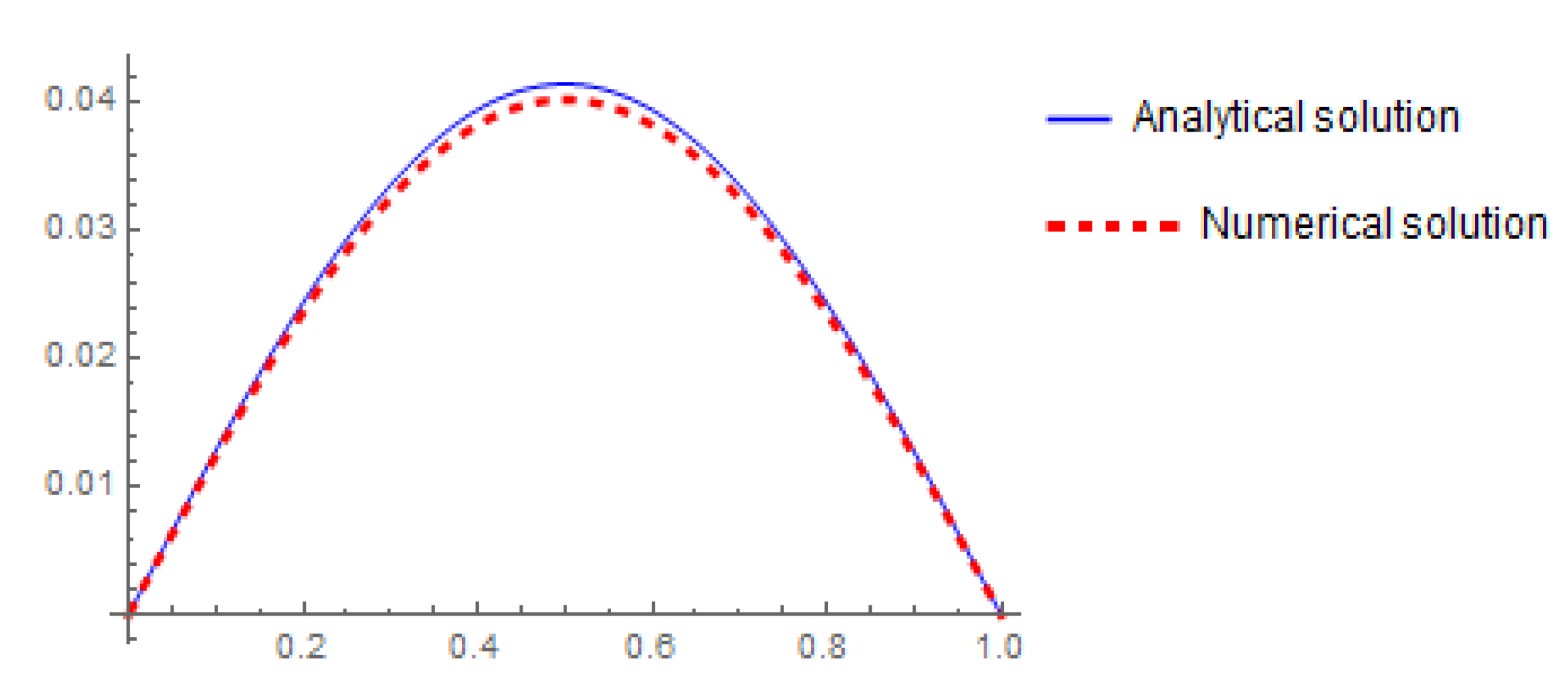
Figure 1. The comparison of the analytical solution with the numerical solution obtained by LHPM for α = 1.47 , t = 1 .
Mathematics 08 01154 g001