Wave-Structure Interaction for a Stationary Surface-Piercing Body Based on a Novel Meshless Scheme with the Generalized Finite Difference Method

Abstract

The wave-structure interaction for surface-piercing bodies is a challenging problem in both coastal and ocean engineering. In the present study, a two-dimensional numerical wave flume that is based on a newly-developed meshless scheme with the generalized finite difference method (GFDM) is constructed in order to investigate the characteristics of the hydrodynamic loads acting on a surface-piercing body caused by the second-order Stokes waves. Within the framework of the potential flow theory, the second-order Runge-Kutta method (RKM2) in conjunction with the semi-Lagrangian approach is carried out to discretize the temporal variable of governing equations. At each time step, the GFDM is employed to solve the spatial variable of the Laplace’s equation for the deformable computational domain. The results show that the developed numerical method has good performance in the simulation of wave-structure interaction, which suggests that the proposed “RKM2-GFDM” meshless scheme can be a feasible tool for such and more complicated hydrodynamic problems in practical engineering.

1. Introduction

Surface-piercing structures are widely employed in both coastal and ocean engineering, such as fixed or floating breakwater, porous membranes, and net-type structures, and hybrid breakwater-WEC system [1,2,3]. It is imperative to investigate the hydrodynamic loads acting on the body surface, as well as the wave pattern surrounding these structures. In the past few years, the meshless method has been developed rapidly to overcome the disadvantages of traditional numerical methods. Meshless methods, such as the Trefftz method [4,5,6,7,8,9,10], the smoothed particle hydrodynamics (SPH) [11,12,13,14,15,16], the method of fundamental solutions (MFS) [17,18,19,20,21], and the generalized finite difference method (GFDM) [22,23,24,25,26,27,28] are widely used by both academia and industry. The GFDM, a true mesh-free numerical scheme, was proposed by Benito et al. in 2001 [22]. They derived the explicit equations of the GFDM while using the moving-least-squares approach. Benito et al. [22,23] also analyzed the influence of some critical parameters of the method on numerical accuracy, as well as successfully solved the parabolic and hyperbolic equations while using the GFDM. In their developed numerical scheme, the spatial derivatives can be expressed as a linear-combined system of function values using various weighting coefficients, which makes the GFDM an easy-to-program meshless scheme as compared with other numerical methods.

In recent years, the GFDM has been successfully employed for the prediction of some classical hydrodynamic issues, such as the propagation of nonlinear water waves [29], sloshing phenomenon in a tank for different filling conditions [30], Boussinesq-type equations in costal engineering [31], and wave pattern surrounding the multiple-bottom seated-cylinder-array structures [32]. Nevertheless, the GFDM has hardly been carried out to calculate the hydrodynamic loads of marine structures so far. In our previous investigation [29], a two-dimensional (2D) numerical wave flume (NWF) was constructed based on the GFDM combining with the second-order Runge–Kutta method (RKM2) and the semi-Lagrangian approach (SLA). Three numerical examples regarding the temporal evolution of nonlinear water waves are studied in order to validate the accuracy and stability of the proposed meshless scheme. The results showed that the GFDM has satisfactory accuracy in the prediction of the propagation of nonlinear water waves, and suggested that the developed numerical method has great potential for more complicated applications in practical engineering.

In the present study, based on the pre-developed 2D NWF, the meshless GFDM is adopted again to investigate the problem of wave-structure interaction between the nonlinear water wave and a stationary surface-piercing body. In Section 2, the governing equations and boundary conditions of the developed NWF are illustrated. In Section 3, the meshless scheme combining with the RKM2 and the SLA are introduced in order to discretize the spatial and temporal variables of the 2D Laplace’s equation. In Section 4, the same problem investigated by Koo et al. [33] is studied as a benchmark of the newly-developed numerical method.

2. Governing Equations and Boundary Conditions

In the present study, a 2D and rectangular NWF for the wave-structures interaction problem is considered. A Cartesian coordinate system $Oxz$ is located at the NWF with the origin being the left-side bottom corner, as shown in Figure 1. The depth of still water and length of the NWF are denoted by h and b, and considered as $\lambda$ and $8\lambda$ in the following calculations, respectively. Besides, the length B of the square structure is set as 0.5 m with the draught d being 0.25 m. As is shown in Figure 1, the boundaries of the NWF are divided into four parts, including the upstream, downstream, impermeable bottom and body surface, and free-surface, which are also denoted by ${\Gamma }_1$, ${\Gamma }_2$, ${\Gamma }_3$, ${\Gamma }_4$, respectively. Besides, two sponge layers are employed at the upstream and downstream boundaries with damping length being $2\lambda$.

2.1. Governing Equations

Under the assumptions of the potential flow, the flow field investigated in the present study can be considered as the inviscid, incompressible, and irrotational fluid, which means that the developed NWF is governed by the 2D Laplace’s equation and the velocity potential can thus be given as

$${\nabla }^2\Phi =\frac{{\partial }^2\Phi }{\partial x^2}+\frac{{\partial }^2\Phi }{\partial z^2}=0,\left(x,z\right)\in \Omega ,$$

(1)

where $\Phi \left(x,z;t\right)$ is the velocity potential, $\Omega$ the deformable computational domain causing by the dynamic free-surface.

2.2. Impermeable and Free-Surface Boundary Condition

The flat and rigid bottom of the NWF and the body surface ${\Gamma }_3$ are considered as the impermeable boundaries, which means that both the bottom and body surface satisfy the so-called no-flux condition, such that

$${\left.\frac{\partial \Phi }{\partial n}\right|}_{{\Gamma }_3}=\frac{\partial \Phi }{\partial x}{n}_x+\frac{\partial \Phi }{\partial z}{n}_z=0,$$

(2)

where n is the unit outward normal vector along the impermeable boundary. Along the free-surface ${\Gamma }_4$, the kinematic and dynamic boundary conditions, respectively, are written as

$$\begin{array}{c}{\left.\frac{\partial \eta }{\partial t}\right|}_{z=\eta +h}=\frac{\partial \Phi }{\partial z}-\frac{\partial \Phi }{\partial x}\frac{\partial \eta }{\partial x},\end{array}$$

(3)

$$\begin{array}{c}{\left.\frac{\partial \Phi }{\partial t}\right|}_{z=\eta +h}=-\frac{1}{2}\left[{\left(\frac{\partial \Phi }{\partial x}\right)}^2+{\left(\frac{\partial \Phi }{\partial z}\right)}^2\right]-g\eta ,\end{array}$$

(4)

where g is the acceleration of gravity, $\eta \left(x;t\right)$ the free-surface elevation and vertically calculated above the still water plane $\eta =0$. The kinematic boundary condition Equation (3) illustrates that the dynamic evolution of the free-surface satisfies the non-breaking condition while the dynamic boundary condition Equation (4) represents that the pressure on the free-surface is equal to the atmospheric pressure.

2.3. Wave-Generating Boundary Condition

As is shown in Figure 1, the upstream boundary ${\Gamma }_1$ is considered as the wave-making condition, which means that the wave propagating along x-direction is generated by imposing horizontal velocity, such that

$${\left.\frac{\partial \Phi }{\partial x}\right|}_{x=0}=U\left(z;t\right),$$

(5)

where $U\left(z;t\right)$ is the velocity function that can be obtained at different physical conditions. In the present study, $U\left(z;t\right)$ is employed according to the analytical solutions of second-order Stokes wave and it is expressed as

$${\left.\frac{\partial \Phi }{\partial x}\right|}_{x=0}=\left[\frac{gkH}{2\omega }\frac{cosh\left(kz\right)}{cosh\left(kh\right)}cos\left(\omega t\right)\right.+\left.\frac{3\omega k{H}^2}{16}\frac{cosh\left(2kz\right)}{{sinh}^4\left(kh\right)}cos\left(2\omega t\right)\right],$$

(6)

where H, $\omega$, and k are wave height, angular frequency, and wave number, respectively. The incident wave should be generated gradually with a so-called ramping function $R_m\left(t\right)$ in order to avoid numerical instability. Following the same method using by Zhang et al. [29], the $R_m\left(t\right)$ is adopted in the present study, given as

$$Rm\left(t\right)=\left\{\begin{array}{cc}{\displaystyle \frac{1}{2}}\left[1-cos\left({\displaystyle \frac{\pi t}{T_m}}\right)\right]\hfill & t\le T_m\hfill \\ 1\hfill & t>T_m\hfill \end{array}\right.,$$

(7)

where $T_m$ is the modulation time and it is set to be twice of wave period T in the following numerical simulations. Consequently, the upstream boundary condition should be re-formulated as

$${\left.\frac{\partial \Phi }{\partial x}\right|}_{x=0}=R_m\left(t\right)U\left(z;t\right).$$

(8)

2.4. Wave-Absorbing Boundary Condition

The phenomenon of wave reflection can be activated and thus affect the propagation of the incident wave if no numerical dissipation is carried out in order to absorb the wave energy. In the present study, two sponge layers are employed to avoid numerical divergence due to the wave reflection, which means that the vertical velocity of fluid particles is damped by a pre-defined mathematical constraint when the reflected waves transport into the sponge layer. Consequently, we adopt two damping coefficients for the upstream and downstream boundaries, defined as

$$\begin{array}{c}{\nu }_1\left(x\right)=\left\{\begin{array}{cc}{\alpha }_{s1}\omega \left[{\displaystyle \frac{x-{\beta }_1\lambda }{{\beta }_1\lambda }}\right]\hfill & x\le {\beta }_1\lambda \hfill \\ 0\hfill & x>{\beta }_1\lambda \hfill \end{array}\right.,\end{array}$$

(9)

$${\nu }_2\left(x\right)=\left\{\begin{array}{cc}{\alpha }_{s2}\omega \left[{\displaystyle \frac{x-\left(b-{\beta }_2\right)\lambda }{{\beta }_2\lambda }}\right]\hfill & x\ge b-{\beta }_2\lambda \hfill \\ 0\hfill & x<b-{\beta }_2\lambda \hfill \end{array}\right.,$$

(10)

where ${\nu }_1\left(x\right)$ and ${\nu }_2\left(x\right)$ are the damping coefficient of the upstream and downstream sponge layer, respectively. ${\beta }_1$, ${\beta }_2$ the length factor and ${\alpha }_{s1}$, ${\alpha }_{s2}$ the tuning factor of the sponge layers. Considering the sponge layers Equations (9) and (10), the free-surface kinematic condition Equation (3) and dynamic condition Equation (4) should be modified as

$$\begin{array}{c}{\left.\frac{\partial \eta }{\partial t}\right|}_{z=\eta +h}=\frac{\partial \Phi }{\partial z}-\frac{\partial \Phi }{\partial x}\frac{\partial \eta }{\partial x}-{\nu }_1\left(x\right)\left(\eta -{\eta }_a\right)-{\nu }_2\left(x\right)\eta ,\end{array}$$

(11)

$$\begin{array}{c}{\left.\frac{\partial \Phi }{\partial t}\right|}_{z=\eta +h}=-\frac{1}{2}\left[{\left(\frac{\partial \Phi }{\partial x}\right)}^2+{\left(\frac{\partial \Phi }{\partial z}\right)}^2\right]-g\eta -{\nu }_1\left(x\right)\left(\Phi -{\varphi }_a\right)-{\nu }_2\left(x\right)\Phi ,\end{array}$$

(12)

where ${\eta }_a$ and ${\varphi }_a$, respectively, are the analytical solutions of free-surface elevation and the velocity potential, which can be expressed as

$$\begin{array}{c}{\eta }_a=\frac{H}{2}cos\left(kx-\omega t\right)+\frac{2+cosh\left(2kh\right)}{4{sinh}^3\left(kh\right)}cos\left[2\left(kx-\omega t\right)\right],\end{array}$$

(13)

$$\begin{array}{c}{\varphi }_a=\frac{Hg}{2\omega }\frac{cosh\left(kz\right)}{cosh\left(kh\right)}sin\left(kx-\omega t\right)+\frac{3H^2\omega }{32}\frac{cosh\left(2kz\right)}{{sinh}^4\left(kh\right)}sin\left[2\left(kx-\omega t\right)\right].\end{array}$$

(14)

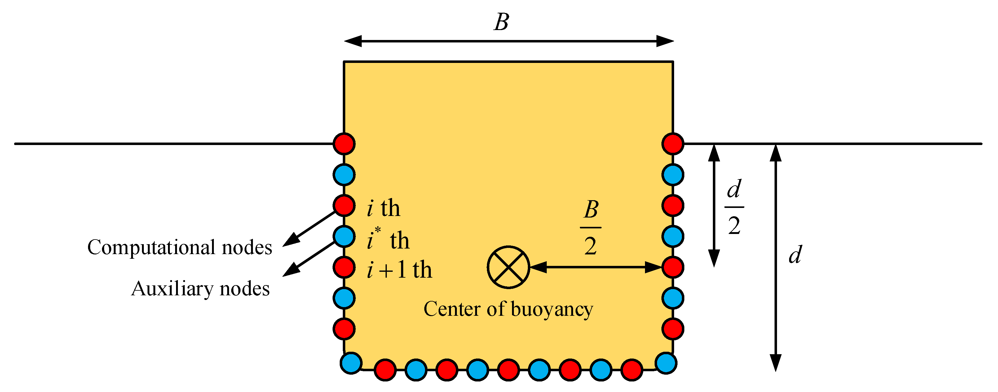
2.5. Hydrodynamics Load of Stationary Structure

As is shown in Figure 2, the nodes that are distributed on the body surface are divided into two type as the computational nodes (red) and auxiliary nodes (blue). The computational nodes are employed to calculate the pressure acting on the ith node, while the adjacent auxiliary nodes $i^{*}$ are adopted to derive the final hydrodynamic loads. In the present study, Bernoulli’s equation is used to calculate the pressure acting on the body surface, which yields

$$P_i^n=-\rho g{\eta }_i^n-\rho \frac{\partial {\Phi }_i^n}{\partial t}-\frac{1}{2}\rho {|\nabla {\Phi }_i^n|}^2,$$

(15)

where $P_i^n$ is the pressure of ith node at n time step and the vector of pressure can be expressed as

$${\mathbf{P}}_i^n=P_i^n{\mathit{n}}_i=P_{i,x}^n\mathit{i}+P_{i,z}^n\mathit{k},$$

(16)

where $\mathit{i}$ and $\mathit{k}$ are the unit vectors along the x- and z-axes, respectively. ${\mathit{n}}_i$ is the unit outward normal vectors along the impermeable body surface for the ith node. The time derivative of velocity potential $\partial {\Phi }_i^n/\partial t$ in Equation (15) is solved using the backward difference scheme, such that

$$\frac{\partial {\Phi }_i^n}{\partial t}=\frac{{\Phi }_i^n-{\Phi }_i^{n-1}}{\mathsf{\Delta }t}.$$

(17)

The gradient of velocity potential $\nabla {\Phi }_i^n$ can be obtained by the GFDM illustrated in Section 3 at each time step and it is written as

$$\nabla {\Phi }_i^n=\frac{\partial {\Phi }_i^n}{\partial x}\mathit{i}+\frac{\partial {\Phi }_i^n}{\partial z}\mathit{k}.$$

(18)

Once $\partial {\Phi }_i^n/\partial t$ and $\nabla {\Phi }_i^n$ are derived, the pressure of the $i^{*}$th node $P_{i^{*}}^n$ can be calculated by the algebraic mean from its adjacent i th and $i+1$ th nodes, which yield

$${\mathit{P}}_{i^{*}}^n=\frac{{\mathit{P}}_i^n+{\mathit{P}}_{i+1}^n}{2}.$$

(19)

The horizontal force $F_{i^{*},x}^n$ and vertical force $F_{i^{*},z}^n$ acting on the body surface for $i^{*}$th node at n time step can be obtained by the dot product

$${\mathit{F}}_{i^{*}}^n={\overline{\mathit{P}}}_{i^{*},x}^n·{\mathit{S}}_{i^{*},x}^n={\overline{P}}_{i^{*},x}^n|S_{i^{*},x}^n|\mathit{i}+{\overline{P}}_{i^{*},z}^n\left|S_{i^{*},z}^n\right|\mathit{k}=F_{i^{*},x}^n\mathit{i}+F_{i^{*},z}^n\mathit{k},$$

(20)

where ${\mathit{S}}_{i^{*}}^n=S_{i^{*}}^n{\mathit{n}}_i=|S_{i^{*},x}^n|\mathit{i}+|S_{i^{*},z}^n|\mathit{k}$ is the area of projection of the body surface along the x- and z- axes. In the present study, ${\mathit{S}}_{i^{*}}^n$ represents the length between two adjacent nodes, because the investigated object is a 2D structure. Consequently, the hydrodynamic force acting on the body surface is obtained by

$$\sum _{i^{*}=1}^{n_{sb}}{\mathit{F}}_{i^{*}}^n=\sum _{i^{*}=1}^{n_{sb}}{F}_{i^{*},x}^n\mathit{i}+\sum _{i^{*}=1}^{n_{sb}}{F}_{i^{*},z}^n\mathit{k},$$

(21)

where $n_{sb}$ is the total numbers of auxiliary nodes. The moment acting on the body surface for the $i^{*}$th node at n time step, according to its definition, can be obtained by the cross product

$$M_{i^{*}}^n={\mathit{r}}_{i^{*}}^n\times {\mathit{F}}_{i^{*}}^n,$$

(22)

where ${\mathit{r}}_{i^{*}}^n$ is the distance between the $i^{*}$th node and the center of buoyancy of the fixed body. Finally, the moment acting on the body surface can be given as

$$\sum _{i^{*}=1}^{n_{sb}}{\mathit{M}}_{i^{*}}^n=\sum _{i^{*}=1}^{n_{sb}}\left({\mathit{r}}_{i^{*}}^n\times {\mathit{F}}_{i^{*}}^n\right).$$

(23)

3. Numerical Methods

3.1. Temporal Discretization

In the present study, the SLA transform is adopted to modify the full Lagrangian equations Equations (3) and (4) for prevent the nodes from escaping out of the deformable computational domain, which means that the fluid particles at free-surface can only move vertically, such that

$$\mathit{u}=0\mathit{i}+\frac{\mathrm{D}\eta }{\mathrm{D}t}\mathit{k},$$

(24)

where $\mathit{u}$ is the vertical velocity of arbitrary fluid particles at free-surface, $\mathrm{D}/ \mathrm{D}t$ the material derivative given as

$$\frac{\mathrm{D}}{\mathrm{D}t}=\frac{\partial }{\partial t}+\mathit{v}·\nabla .$$

(25)

Substituting $\eta (x;t)$ and $\Phi (x,z;t)$ into Equation (25), the following expressions are obtained

$$\begin{array}{c}\frac{\mathrm{D}\eta }{\mathrm{D}t}=\frac{\partial \eta }{\partial t},\frac{\mathrm{D}\Phi }{\mathrm{D}t}=\frac{\partial \Phi }{\partial t}+\frac{\partial \Phi }{\partial z}\frac{\mathrm{D}\eta }{\mathrm{D}t}.\end{array}$$

(26)

According to Equation (26), the SLA forms of Equations (11) and (12) are written as

$$\begin{array}{c}{\left.\frac{\mathrm{D}\eta }{\mathrm{D}t}\right|}_{z=\eta +h}=\frac{\partial \Phi }{\partial z}-\frac{\partial \eta }{\partial x}\frac{\partial \Phi }{\partial x}-{\nu }_1\left(x\right)\left(\eta -{\eta }_a\right)-{\nu }_2\left(x\right)\eta ,\end{array}$$

(27)

$$\begin{array}{c}{\left.\frac{\mathrm{D}\Phi }{\mathrm{D}t}\right|}_{z=\eta +h}=-\frac{1}{2}\left[{\left(\frac{\partial \Phi }{\partial x}\right)}^2+{\left(\frac{\partial \Phi }{\partial z}\right)}^2\right]-g\eta +\frac{\partial \Phi }{\partial z}\left(\frac{\partial \Phi }{\partial z}-\frac{\partial \eta }{\partial x}\frac{\partial \Phi }{\partial x}\right)-{\nu }_1\left(x\right)\left(\Phi -{\Phi }_a\right)-{\nu }_2\left(x\right)\Phi .\end{array}$$

(28)

RKM2 is employed to discretize Equations (27) and (28) for better numerical stability in calculations. At the beginning of a simulation, the derivative $F_1={\left.\frac{\mathrm{D}\eta }{\mathrm{D}t}\right|}_{z=\eta +h}$ and $F_2={\left.\frac{\mathrm{D}\Phi }{\mathrm{D}t}\right|}_{z=\eta +h}$ can be solved according to the free-surface boundary condition, and the numerical scheme with respect to time integration is thus yielded

$$\begin{array}{c}{\eta }^{*}={\eta }^n+F_1^n\mathsf{\Delta }t,\end{array}$$

(29)

$$\begin{array}{c}{\Phi }^{*}={\Phi }^n+F_2^n\mathsf{\Delta }t,\end{array}$$

(30)

where the superscripts n and * denote, respectively, the physical values at $t_n$ and the temporary time steps. Once the temporary physical values are obtained, the time derivative of the free-surface at $t_n$ can be calculated after trigging the proportionally re-distribution of nodes along every vertical line. The numerical process can be advanced into next time-layer in the same manner, and the physical values at $t_{n+1}$, on the basis of the RKM2 algorithm, can be given as

$$\begin{array}{c}{\eta }^{n+1}=\frac{1}{2}\left[\left({\eta }^{*}+F_1^{*}\mathsf{\Delta }t\right)+{\eta }^n\right],\end{array}$$

(31)

$$\begin{array}{c}{\Phi }^{n+1}=\frac{1}{2}\left[\left({\Phi }^{*}+F_2^{*}\mathsf{\Delta }t\right)+{\Phi }^n\right].\end{array}$$

(32)

3.2. Spatial Discretization

We develope a spatial numerical scheme based on the GFDM for sovling 2D Laplace’s equation at each time steps. In order to obtain the explicit GFDM equation systems, an arbitrary cloud of nodes, as is shown in Figure 3, is scattered in the deformable computational domain. On defining the composition central node (denoted by ith) with a set of nodes (also known as the star) surrounding the same, assume that ${\Phi }_i$ is the value of the function of the ith node of the star, and ${\Phi }_j(j=1,\cdots ,n_s)$ the value of the function at the rest of nodes. Subsequently, according to the Taylor series expansion, the values ${\Phi }_j$ can be expressed as

$${\Phi }_{i,j}={\Phi }_i+x_{ij}{\left.\frac{\partial \Phi }{\partial x}\right|}_i+z_{ij}{\left.\frac{\partial \Phi }{\partial z}\right|}_i+\frac{x_{ij}^2}{2}{\left.\frac{{\partial }^2\Phi }{\partial x^2}\right|}_i+\frac{z_{ij}^2}{2}{\left.\frac{{\partial }^2\Phi }{\partial z^2}\right|}_i+x_{ij}{z}_{ij}{\left.\frac{{\partial }^2\Phi }{\partial x\partial z}\right|}_i+\cdots \left(j=1,\cdots ,n_s\right).$$

(33)

In the GFDM, the moving-least squares approach is carried out in order to obtain the expressions of spatial derivatives at every node. Because the governing equation is a second-order partial differential equation, we implement the second-order Taylor series to express the distribution of solution within the star. When the Equation (33) is truncated by the second-order derivative, it is then possible to define the $B\left(\Phi \right)$ function as

$$B\left(\Phi \right)=\sum _{j=1}^{j=n_s}{\left[w\left(x_{ij},z_{ij}\right)T_{ij}\left(\Phi \right)\right]}^2,$$

(34)

where $T_{ij}\left(\Phi \right)$ is the residual function, given as

$$T_{ij}\left(\Phi \right)={\Phi }_i-{\Phi }_{i,j}+x_{ij}{\left.\frac{\partial \Phi }{\partial x}\right|}_i+z_{ij}{\left.\frac{\partial \Phi }{\partial z}\right|}_i+\frac{x_{ij}^2}{2}{\left.\frac{{\partial }^2\Phi }{\partial x^2}\right|}_i+\frac{z_{ij}^2}{2}{\left.\frac{{\partial }^2\Phi }{\partial z^2}\right|}_i+x_{ij}{z}_{ij}{\left.\frac{{\partial }^2\Phi }{\partial x\partial z}\right|}_i,$$

(35)

where ${\Phi }_i$ and ${\Phi }_{i,j}$ are physical solutions at the ith node and the other $n_s$ nearest nodes, $x_{ij}=x_j^i-x_i$, $z_{ij}=z_j^i-z_i$ the distance between ith node and jth node in the star along x, z direction, $w(x_{ij},z_{ij})$ the so-called weighting function. Furthermore, the quadratic spline is employed as the weighting function $w(x_{ij},z_{ij})$ in the present study [22]:

$$w\left(x_{ij},z_{ij}\right)=\left\{\begin{array}{cc}1-6{\left(\frac{d_{ij}}{d_i^{\max }}\right)}^2+8{\left(\frac{d_{ij}}{d_i^{\max }}\right)}^3-3{\left(\frac{d_{ij}}{d_i^{\max }}\right)}^4\hfill & d_{ij}\le d_i^{\max }\hfill \\ 0\hfill & d_{ij}>d_i^{\max }\hfill \end{array}\right.,$$

(36)

where $d_{ij}=\sqrt{x_{ij}^2+z_{ij}^2}$ is the distance between ith node and jth node of the star, $d_i^{\max }$ the distance between the ith node and the farthest node with the star. We define the partial derivative matrix ${\mathbf{D}}_{\mathbf{u}}$ as

$${\left\{{\mathbf{D}}_{\mathbf{u}}\right\}}_{5\times 1}={\left\{\begin{array}{c}{\left.{\displaystyle \frac{\partial \Phi }{\partial x}}\right|}_i{\left.{\displaystyle \frac{\partial \Phi }{\partial z}}\right|}_i{\left.{\displaystyle \frac{{\partial }^2\Phi }{\partial x^2}}\right|}_i{\left.{\displaystyle \frac{{\partial }^2\Phi }{\partial z^2}}\right|}_i{\left.{\displaystyle \frac{{\partial }^2\Phi }{\partial x\partial z}}\right|}_i\end{array}\right\}}^{\mathrm{T}}.$$

(37)

Consider that the norm $B\left(\Phi \right)$ is minimized with respect to the partial derivative ${\mathbf{D}}_{\mathbf{u}}$, such that

$$\frac{\partial B\left(\Phi \right)}{\partial {\mathbf{D}}_{\mathbf{u}}}=0.$$

(38)

A linear system of algebraic equations, consequently, is yielded

$$\mathbf{A}{\mathbf{D}}_{\mathbf{u}}=\mathbf{b},$$

(39)

where $\mathbf{A}$ is a symmetric matrix. $\mathbf{A}$ and $\mathbf{b}$ is expressed as

$$\mathbf{A}=\left\{\begin{array}{ccccc}\hfill {\displaystyle \sum _{j=1}^{n_s}}{w}_{ij}^2{x}_{ij}^2& {\displaystyle \sum _{j=1}^{n_s}}{w}_{ij}^2{x}_{ij}{z}_{ij}& {\displaystyle \sum _{j=1}^{n_s}}{w}_{ij}^2\frac{x_{ij}^3}{2}\hfill & {\displaystyle \sum _{j=1}^{n_s}}{w}_{ij}^2\frac{x_{ij}{z}_{ij}^2}{2}& {\displaystyle \sum _{j=1}^{n_s}}{w}_{ij}^2{x}_{ij}^2{z}_{ij}\\ \hfill & {\displaystyle \sum _{j=1}^{n_s}}{w}_{ij}^2{z}_{ij}^2& {\displaystyle \sum _{j=1}^{n_s}}{w}_{ij}^2\frac{x_{ij}^2{z}_{ij}}{2}\hfill & {\displaystyle \sum _{j=1}^{n_s}}{w}_{ij}^2\frac{z_{ij}^3}{2}& {\displaystyle \sum _{j=1}^{n_s}}{w}_{ij}^2{x}_{\mathrm{ij}}{z}_{ij}^2\\ \hfill & & {\displaystyle \sum _{j=1}^{n_s}}{w}_{ij}^2\frac{x_{ij}^4}{2}\hfill & {\displaystyle \sum _{j=1}^{n_s}}{w}_{ij}^2\frac{x_{ij}^2{z}_{ij}^2}{4}& {\displaystyle \sum _{j=1}^{n_s}}{w}_{ij}^2\frac{x_{ij}^3{z}_{ij}}{2}\\ \hfill & \mathrm{SYM}& \hfill & {\displaystyle \sum _{j=1}^{n_s}}{w}_{ij}^2\frac{z_{ij}^4}{2}& {\displaystyle \sum _{j=1}^{n_s}}{w}_{ij}^2\frac{x_{ij}{z}_{ij}^3}{2}\\ \hfill & & \hfill & & {\displaystyle \sum _{j=1}^{n_s}}{w}_{ij}^2{x}_{ij}^2{z}_{ij}^2\end{array}\right\},$$

(40)

$$\mathbf{b}=\left\{\begin{array}{c}{\Phi }_i{\displaystyle \sum _{j=1}^{n_s}}{w}_{ij}^2{x}_{ij}-{\displaystyle \sum _{j=1}^{n_s}}{\Phi }_{i,j}{w}_{ij}^2{x}_{ij}\\ {\Phi }_i{\displaystyle \sum _{j=1}^{n_s}}{w}_{ij}^2{z}_{\mathrm{ij}}-{\displaystyle \sum _{j=1}^{n_s}}{\Phi }_{i,j}{w}_{ij}^2{z}_{ij}\\ {\Phi }_i{\displaystyle \sum _{j=1}^{n_s}}{w}_{ij}^2{\displaystyle \frac{x_{ij}^2}{2}}-{\displaystyle \sum _{j=1}^{n_s}}{\Phi }_{i,j}{w}_{ij}^2{\displaystyle \frac{x_{ij}^2}{2}}\\ {\Phi }_i{\displaystyle \sum _{j=1}^{n_s}}{w}_{ij}^2{\displaystyle \frac{z_{ij}^2}{2}}-{\displaystyle \sum _{j=1}^{n_s}}{\Phi }_{i,j}{w}_{ij}^2{\displaystyle \frac{z_{ij}^2}{2}}\\ {\Phi }_i{\displaystyle \sum _{j=1}^{n_s}}{w}_{ij}^2{x}_{ij}{z}_{ij}-{\displaystyle \sum _{j=1}^{n_s}}{\Phi }_{i,j}{w}_{ij}^2{x}_{ij}{z}_{ij}\end{array}\right\}.$$

(41)

The matrix $\mathbf{b}$ can be re-formulated as

$$\mathbf{b}=\mathbf{BQ},$$

(42)

where $\mathbf{Q}$$=\{{\Phi }_i,{\Phi }_{i,1},\cdots ,{\Phi }_{i,ns}\}$ is the total velocity potential at the central ith node and the other $n_s$ nearest nodes within the star. $\mathbf{b}$ is a coefficient matrix and its value is related to the spatial coordinate and weighting function of the $n_s+1$ node within the star of the ith node. Consequently, ${\mathbf{D}}_{\mathbf{u}}$ can be re-written as

$${\mathbf{D}}_{\mathbf{u}}=\left\{\begin{array}{c}{\left.{\displaystyle \frac{\partial \Phi }{\partial x}}\right|}_i\\ {\left.{\displaystyle \frac{\partial \Phi }{\partial z}}\right|}_i\\ {\left.{\displaystyle \frac{{\partial }^2\Phi }{\partial x^2}}\right|}_i\\ {\left.{\displaystyle \frac{{\partial }^2\Phi }{\partial z^2}}\right|}_i\\ {\left.{\displaystyle \frac{{\partial }^2\Phi }{\partial x\partial z}}\right|}_i\end{array}\right\}={\mathbf{A}}^{-\mathbf{1}}\mathbf{b}={\mathbf{A}}^{-\mathbf{1}}\mathbf{B}\mathbf{Q}=\mathbf{D}{\left\{\begin{array}{c}{\Phi }_i\\ {\Phi }_{i,1}\\ {\Phi }_{i,2}\\ {\Phi }_{i,3}\\ ⋮\\ {\Phi }_{i,n_s}\end{array}\right\}}_{\left({\mathbf{n}}_{\mathbf{s}}+\mathbf{1}\right)\times \mathbf{1}}.$$

(43)

It is obvious that the spatial derivative ${\mathbf{D}}_{\mathbf{u}}$ at the ith node are transformed into a linear algebraic system of $n_s+1$ physical values with a different weighting function. The coefficient matrix $\mathbf{D}={\mathbf{A}}^{-\mathbf{1}}\mathbf{B}$ depends on the total numbers of nodes, the weighting function, and the spatial coordinate of the nodes in the star. In order to clearly illustrate the numerical scheme of the spatial derivative at the ith node, above equation can be recast as

$$\begin{array}{cc}\hfill {\left.{\displaystyle \frac{\partial \Phi }{\partial x}}\right|}_i& =e_{1,1}^i{\Phi }_i+\sum _{j=1}^{n_s}{e}_{1,j+1}^i{\Phi }_{i,j},\hfill \end{array}$$

(44)

$$\begin{array}{cc}\hfill {\left.{\displaystyle \frac{\partial \Phi }{\partial z}}\right|}_i& =e_{2,1}^i{\Phi }_i+\sum _{j=1}^{n_s}{e}_{2,j+1}^i{\Phi }_{i,j},\hfill \end{array}$$

(45)

$$\begin{array}{cc}\hfill {\left.{\displaystyle \frac{{\partial }^2\Phi }{\partial x^2}}\right|}_i& =e_{3,1}^i{\Phi }_i+\sum _{j=1}^{n_s}{e}_{3,j+1}^i{\Phi }_{i,j},\hfill \end{array}$$

(46)

$$\begin{array}{cc}\hfill {\left.{\displaystyle \frac{{\partial }^2\Phi }{\partial z^2}}\right|}_i& =e_{4,1}^i{\Phi }_i+\sum _{j=1}^{n_s}{e}_{4,j+1}^i{\Phi }_{i,j},\hfill \end{array}$$

(47)

$$\begin{array}{cc}\hfill {\left.{\displaystyle \frac{{\partial }^2\Phi }{\partial x\partial z}}\right|}_i& =e_{5,1}^i{\Phi }_i+\sum _{j=1}^{n_s}{e}_{5,j+1}^i{\Phi }_{i,j},\hfill \end{array}$$

(48)

where ${\left\{e_{k,j}\right\}}_{j=1}^{n_s+1}\left(k=1,\cdots ,5\right)$ is weighting coefficients corresponding to the nodes and the star, which can be numerically calculated while using the above developed numerical method. It is obvious that the numerical procedures of the moving-least square method and the Taylor series to derive the expressions of derivatives Equations (44)–(48) are easy-to-program. Every node inside the computational domain and along the boundaries should be considered as the ith nodes in order to derive the expressions of derivatives by repeating the numerical procedures of Equations (33)–(43). Once the expressions of derivatives at every node are acquired, a simple approach of collocation is implemented in order to obtain the GFDM solution. A sparse system of linear algebraic equations can be yielded by enforcing the satisfactions of governing equation at every interior node and of boundary conditions at every boundary node. The numerical solutions can be efficiently acquired while the resultant sparse system of linear algebraic equations is solved. The above-mentioned numerical procedures of collocation are almost identical to the classical finite difference method, but neither coordinate transformation nor orthogonal grid are required in the GFDM. Thus, it is evident that the GFDM, a newly-developed meshless method, is very suitable for solving the wave-structure interaction for a stationary surface-piercing body.

4. Numerical Results and Discussion

A physical problem regarding the interaction between the second-order Stokes wave and the single surface-piercing body is studied in order to validate the accuracy and stability of the proposed meshless scheme. In the present study, the meshless NWF is developed and employed in order to calculate a series of harmonic hydrodynamic loads acting on the body surface. All of the obtained results except independence validations are post-processed with the fast Fourier transform (FFT) to derive the harmonic hydrodynamic loads while using the steady-state portion of time history curves, such that

$$f\left(t\right)=\frac{a_0}{2}+\sum _{n=1}^{\infty }\left(a_{n}cos{\omega }_{n}t+b_{n}sin{\omega }_{n}t\right),$$

(49)

where $a_0$, $a_n$, $b_n$ are Fourier coefficients, ${\omega }_n$ the angular frequency of nth order harmonic component, $f\left(t\right)$ the time history curves of hydrodynamic loads $F_x$, $F_z$ and $M_y$. Equation (49) can be modified as

$$\begin{array}{cc}\hfill f\left(t\right)& =\frac{a_0}{2}+\sum _{n=1}^{\infty }\sqrt{a_n^2+b_n^2}\left(\frac{a_n}{\sqrt{a_n^2+b_n^2}}cos{\omega }_{n}t+\frac{b_n}{\sqrt{a_n^2+b_n^2}}sin{\omega }_{n}t\right)\hfill \\ \hfill & =\frac{a_0}{2}+\sum _{n=1}^{\infty }\sqrt{a_n^2+b_n^2}\left(cos{\theta }_{n}cos\omega t+sin{\theta }_{n}sin\omega t\right)\hfill \\ \hfill & =C_0+\sum _{n=1}^{\infty }{A}_{n}cos\left({\omega }_{n}t-{\theta }_n\right),\hfill \end{array}$$

(50)

where $C_0$ is a constant depending on different case conditions. $A_n=\sqrt{a_n^2+b_n^2}$ the amplitude of nth order harmonic component, ${\theta }_n$ the phase angle.

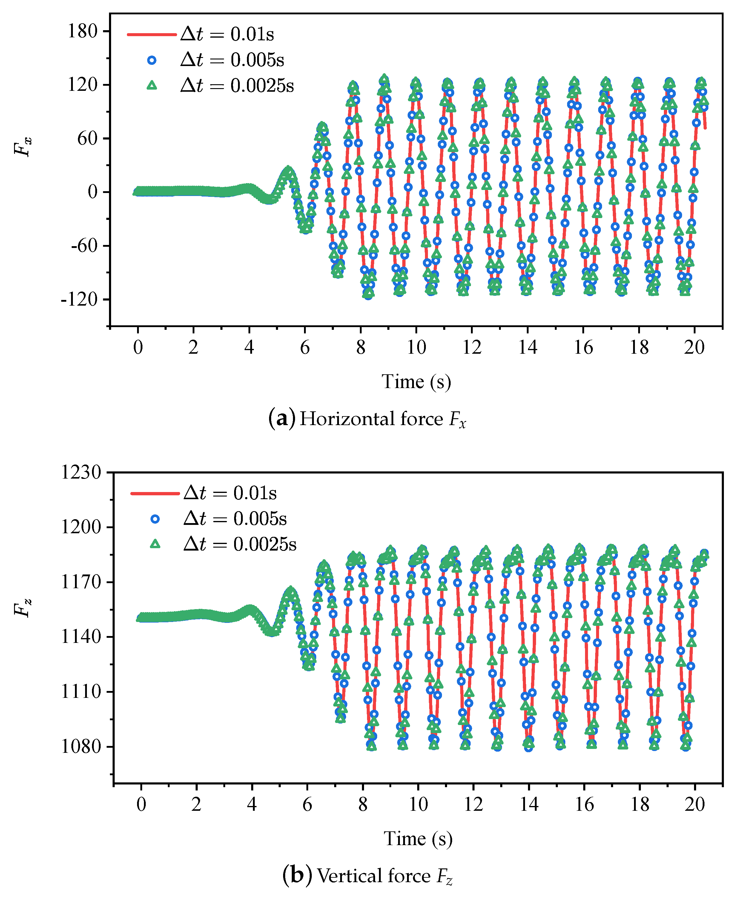
4.1. Independence Validations

It is necessary to determine the most suitable time step $\mathsf{\Delta }t$ and number of nodes N for the newly-developed meshless scheme, which means that a benchmark of independence validations must be implemented before the investigation.

Table 1. Numerical parameters of numbers total nodes N, spaces of nodes along x and z axes ($\mathsf{\Delta }x$ and $\mathsf{\Delta }z$), time increment ($\mathsf{\Delta }t$) and the simulation duration (t) of five cases for the validation of convergence and stability.

Case	N	$\mathbf{\Delta }\mathit{x}$	$\mathbf{\Delta }\mathit{z}$	$\mathbf{\Delta }\mathit{t}$	t
No.01	280,380	$0.01\mathrm{m}$	$0.01\mathrm{m}$	$0.01\mathrm{s}$	15 T
No.02	280,380	$0.01\mathrm{m}$	$0.01\mathrm{m}$	$0.005\mathrm{s}$	15 T
No.03	280,380	$0.01\mathrm{m}$	$0.01\mathrm{m}$	$0.0025\mathrm{s}$	15 T
No.04	345,462	$0.009\mathrm{m}$	$0.009\mathrm{m}$	$0.01\mathrm{s}$	15 T
No.05	437,616	$0.008\mathrm{m}$	$0.008\mathrm{m}$	$0.01\mathrm{s}$	15 T

shows the information of the time step $\mathsf{\Delta }t$ and total numbers of nodes N for the benchmark. The cases of No.01, No.02, and No.03 are carried out with N = 28,0380 and $\mathsf{\Delta }t=0.01\mathrm{s},0.005\mathrm{s},0.0025\mathrm{s}$ for the time step independence validations, while the cases of No.01, No.04, and No.05 are carried out with $\mathsf{\Delta }t=0.01\mathrm{s}$ and $N=$ 280,380, 345,462, 437,and 616 for the nodes independence validations. The simulating duration t, wave length $\lambda$, and wave height H are considered with 15 T, 2.0 m, and 0.07 m, respectively. Because the wave gauges G1 will not be affected by the reflected wave, the time history curve of wave gauge G1 is adopted to validate the accuracy of the incident second-order Stokes wave. It can be observed from Figure 4 that the simulated wave elevation is in perfect agreement with the analytical solutions of the second-order Stokes wave, which means that the developed NWF can generate high-accuracy nonlinear water waves for further investigations. Figure 5 and Figure 6 shows the numerical results of the benchmark of independence validations. When the calculation reaches a stable state, the hydrodynamic loads $F_x$, $F_z$, and $M_y$ of each numerical example periodically fluctuate with time, and show almost the same trend, indicating that each numerical case has converged on the given time steps and total numbers of nodes. It is demonstrated that the proposed numerical method has great accuracy and stability for such a problem. According to the simulation results of the benchmark, $\mathsf{\Delta }t=0.01\mathrm{s}$, and $N=$ 280,380 are chosen for the following investigations.

4.2. Hydrodynamic Loads

Numerical case conditions are considered to be the same as the investigation by Koo et al. [33] to benchmark our newly-proposed numerical methods.

Table 2. Numerical parameters of twelve cases for simulation of wave-structure interaction of a surface-piercing body.

Case	Wave Period (s)	Wave Frequency (rad/s)	Wave Length (m)	Wave Steepness		$\mathit{\xi }={\displaystyle \frac{{\mathit{\omega }}^2\mathit{B}}{2\mathit{g}}}$
				$\mathit{H}=\mathbf{0.07}\mathrm{m}$	$\mathit{H}=\mathbf{0.01}\mathrm{m}$
No.01	$0.8003$	$7.8510$	$1.0$	$1/143$	$1/100$	$1.5708$
No.02	$0.8767$	$7.1669$	$1.2$	$1/171$	$1/120$	$1.3090$
No.03	$0.9469$	$6.6355$	$1.4$	$1/200$	$1/140$	$1.1220$
No.04	$1.0123$	$6.2068$	$1.6$	$1/229$	$1/160$	$0.9817$
No.05	$1.0737$	$5.8519$	$1.8$	$1/257$	$1/180$	$0.8727$
No.06	$1.1318$	$5.5515$	$2.0$	$1/286$	$1/200$	$0.7854$
No.07	$1.1870$	$5.2933$	$2.2$	$1/314$	$1/220$	$0.7140$
No.08	$1.2398$	$5.0679$	$2.4$	$1/343$	$1/240$	$0.6545$
No.09	$1.3392$	$4.6917$	$2.8$	$1/400$	$1/280$	$0.5610$
No.10	$1.4972$	$4.1966$	$3.5$	$1/500$	$1/350$	$0.4488$
No.11	$1.5601$	$4.0274$	$3.8$	$1/543$	$1/380$	$0.4134$
No.12	$1.6401$	$3.8310$	$4.2$	$1/600$	$1/420$	$0.3740$

shows all considered numerical cases. The wave length $\lambda$ ranges from 1.0 m to 4.2 m with two different wave heights $H=0.01\mathrm{m}$ and $H=0.07\mathrm{m}$. Figure 7 shows the comparison of the first-order harmonic hydrodynamic loads acting on the body surface with other pre-investigated data, including the analytical solutions [34], experimental results [35], and two BEM results [33,36]. The calculated first-order harmonic hydrodynamic loads $F_x$ and $F_z$, as is shown in Figure 7d,e, are in good agreement with other pre-obtained results. However, the first-order harmonic moment $M_y$ is slightly over-predicted at low $\xi$ as compared with the analytical solutions and experimental implemention. But it can be seen from Figure 7f that the calculated results is also in good agreement with the BEM results [36] at low $\xi$. It can be observed that the GFDM and BEM both over-predict the moment acting on the body surface. The main reason for this phenomenon is that we suppose the spatial coordinate of the center of rotation is fixed and equals the center of buoyancy. The traditional BEM is under the same assumption. However, in the real physical world, the center of buoyancy moves periodically at the static-balanced position. Accordingly, the experiment results are in good agreement with the analytical solutions, while the numerical results by the BEM and the GFDM may show some deviations due to the fixed-rotating-center assumption. Another reason may be that the GFDM and the BEM are developed within the framework of potential flow theory, in which the viscous effects, such as shear stress caused by the fluid boundary layer and vortex shedding at edges of the body, are ignored and, thus, cause the errors.

In general, the numerical method proposed in the present study has enough accuracy in the prediction of the first-order harmonic component for a problem regarding the wave-structure interaction. In addition, it can also be observed that the wave steepness has little effect on the results of the dimensionless hydrodynamic loads with various $\xi$, which means that the hydrodynamic loads are linearly and positively correlated with the wave height. Koo et al. [33] also analyzed and discussed the higher harmonic hydrodynamic loads acting on the surface-piercing body. They found that the first-order harmonic component is lager as compared with the second-order and three-order components, and the second-order vertical force $F_z$ may greatly exceed the first-order component at high $\xi$. Figure 8a,c show the first-three harmonic hydrodynamic loads acting on the body surface. The first-order harmonic component contributes most of the hydrodynamic loads, while the second-order harmonic component may exceed the first-order at low $\xi$. The third-order harmonic component has a minimal effect on the hydrodynamic loads. It is seen that the proposed meshless scheme also shows good performance in the prediction of high-order hydrodynamic loads as compared with the BEM results [33].

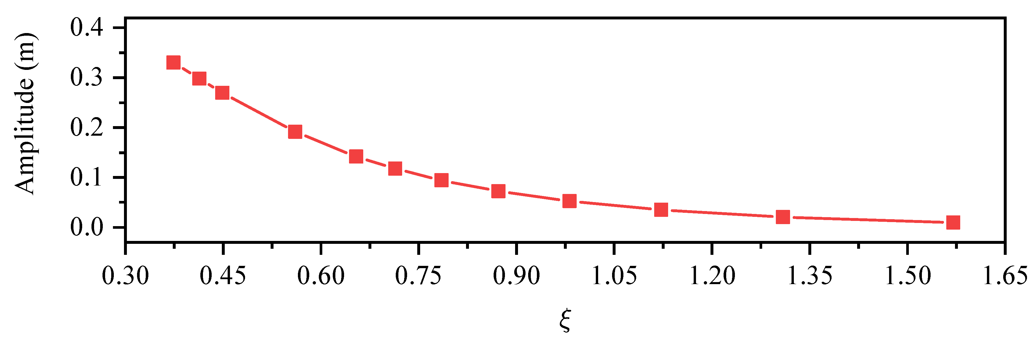
4.3. Transmitted Wave

Figure 9 depicts the temporal evolution of the wave field with wave length $\lambda =1.0\mathrm{m}$ and wave height $H=0.07\mathrm{m}$. At the condition of wave length $\lambda =1.0\mathrm{m}$, the amplitude of the transmitted wave behind the structure is almost zero. However, at large wave length $\lambda =2.0\mathrm{m}$ and weve height $H=0.07\mathrm{m}$, as is shown in Figure 10, the amplitude of the transmitted wave increases obviously. Figure 11 shows the time history curve of the wave elevation under different numerical cases. It is obvious from the figure that the greater the wave length of incident wave, the greater the amplitude of the transmitted wave. This phenomenon can be explained from the viewpoint of wave energy. Mathematically, wave energy $E_w$ can be expressed as

$$E_w=\frac{1}{16}\rho g{H}^2{c}_g,$$

(51)

where $c_g$ is the group velocity and it can be written as $c_g=gT/4\pi$ due to the deep water condition $h=\lambda$ in the present study. Consequently, Equation (51) can be recast as

$$E_w=\frac{1}{16}\rho g{H}^2\left(\frac{gT}{4\pi }\right).$$

(52)

For the developed NWF, the wave energy $E_w$ of the incoming second-order Stokes wave, after interaction with the structure, can be divided into three parts, including the reflected components $E_r$, transmitted components $E_t$, and dissipated components $E_d$, in which the dissipated components $E_d$ are caused by the hydrodynamic loads acting on the body surface. The numerical cases that are shown in Table 2 are designed by different wave lengths with fixed wave height, which means that the wave energy $E_w$ increases in order from No.01 to No.12 because of the fixed wave height and increasing wave length in Equation (52). In order to further investigate the characteristics of the transmitted wave, the FFT technique is again employed to post-process the time history curves of the monitored wave elevation from wave gauge G3 for all of the calculated cases. Figure 12 shows the first-order harmonic amplitude of the transmitted wave elevation with various $\xi$. It can be seen that, as the wave length $\lambda$ increases (the same as $\xi$ decreases), the first-order harmonic amplitude of the transmitted wave also increases. When the wavelength is 4.2 m ($\xi =0.3740$), the amplitude of the transmitted wave even reaches $50\%$ of the incident wave. It is demonstrated that the proposed meshless scheme can accurately capture the transmission effect for the propagation of nonlinear water waves.

5. Conclusions

In the present study, we develop a novel meshless numerical method for the problem with respect to the wave-structure interaction between the nonlinear water waves and a stationary surface-piercing body. Within the framework of the potential flow theory, the RKM2 combining with the SLA is employed to discretize the temporal variable of governing equations. Based on the moving least squares method and the second-order Taylor series expansion, the GFDM is then carried out in order to solve the spatial variable of the Laplace’s equation for the deformable computational domain. The simulated wave elevation, post-processed hydrodynamic loads, as well as the transmitted waves behind the structure are investigated and discussed to validate the accuracy and stability of the proposed meshless scheme. The monitored time-history curve of wave elevation from wave gauge G1 illustrates that the simulated results are in perfectly good agreement with the analytical solutions of the second-order Stokes wave. The hydrodynamic loads acting on the structure for different time steps and total numbers of nodes are obtained in order to validate the stability and convergency of the developed meshless scheme, and the results show that the meshless scheme is stable enough for such problems. Furthermore, hydrodynamic loads acting on the body surface are calculated for different numerical cases with various wave length and wave height, which are compared with the analytical, experimental, and two BEM-based numerical results using the FFT technique. The comparison demonstrates that the first-three harmonic hydrodynamic loads, generally, are also in good agreement with other pre-investigated results. Moreover, the characteristics of the transmitted waves behind the studied surface-piercing body are also consistent with the conclusion derived from the viewpoint of wave energy.

In general, the newly-developed numerical method shows good performance in the simulation of nonlinear wave propagation, hydrodynamic loads acting on the body surface, and the transmission effect due to the existence of a structure. The proposed "RKM2-GFDM" meshless scheme, as is shown in the present study, has great potential for more complicated hydrodynamic problems in practical engineering. In the future, we will continue to modify and improve the proposed meshless scheme for three-dimensional applications and hydrodynamics of the floating surface-piercing body.

References

1. Dai, J.; Wang, C.M.; Utsunomiya, T.; Duan, W. Review of recent research and developments on floating breakwaters. Ocean Eng. 2018, 158, 132–151. [Google Scholar] [CrossRef]
2. Guo, Y.; Mohapatra, S.; Soares, C.G. Review of developments in porous membranes and net-type structures for breakwaters and fish cages. Ocean Eng. 2020, 200, 107027. [Google Scholar] [CrossRef]
3. Zhao, X.; Ning, D.; Zou, Q.; Qiao, D.; Cai, S. Hybrid floating breakwater-WEC system: A review. Ocean Eng. 2019, 186, 106126. [Google Scholar] [CrossRef]
4. Liu, C.S. A modified Trefftz method for two-dimensional Laplace equation considering the domain’s characteristic length. Comput. Model. Eng. Sci. 2007, 21, 53–65. [Google Scholar]
5. Liu, C.S. An effectively modified direct Trefftz method for 2D potential problems considering the domain’s characteristic length. Eng. Anal. Bound. Elem. 2007, 31, 983–993. [Google Scholar] [CrossRef]
6. Chen, J.T.; Wu, C.S.; Lee, Y.T.; Chen, K.H. On the equivalence of the Trefftz method and method of fundamental solutions for Laplace and biharmonic equations. Comput. Math. Appl. 2007, 53, 851–879. [Google Scholar] [CrossRef] [Green Version]
7. Li, Z.C.; Lu, T.T.; Huang, H.T.; Cheng, A.H.D. Trefftz, collocation, and other boundary methods—A comparison. Numer. Methods Partial Differ. Equ. 2007, 23, 93–144. [Google Scholar] [CrossRef]
8. Liu, C.S. A modified collocation Trefftz method for the inverse Cauchy problem of Laplace equation. Eng. Anal. Bound. Elem. 2008, 32, 778–785. [Google Scholar] [CrossRef]
9. Lee, W.M.; Chen, J.T. Scattering of flexural wave in a thin plate with multiple circular holes by using the multipole Trefftz method. Int. J. Solid Struct. 2010, 47, 1118–1129. [Google Scholar] [CrossRef]
10. Liu, C.S.; Atluri, S.N. Numerical solution of the Laplacian Cauchy problem by using a better postconditioning collocation Trefftz method. Eng. Anal. Bound. Elem. 2013, 37, 74–83. [Google Scholar] [CrossRef]
11. Liu, M.B.; Liu, G.R. Smoothed Particle Hydrodynamics (SPH): An Overview and Recent Developments. Arch. Comput. Methods Eng. 2010, 17, 25–76. [Google Scholar] [CrossRef] [Green Version]
12. Xu, R.; Stansby, P.; Laurence, D. Accuracy and stability in incompressible SPH (ISPH) based on the projection method and a new approach. J. Comput. Phys. 2009, 228, 6703–6725. [Google Scholar] [CrossRef]
13. Lee, E.S.; Moulinec, C.; Xu, R.; Violeau, D.; Laurence, D.; Stansby, P. Comparisons of weakly compressible and truly incompressible algorithms for the SPH mesh free particle method. J. Comput. Phys. 2008, 227, 8417–8436. [Google Scholar] [CrossRef]
14. Hu, X.Y.; Adams, N.A. An incompressible multi-phase SPH method. J. Comput. Phys. 2007, 227, 264–278. [Google Scholar] [CrossRef]
15. Hu, X.Y.; Adams, N.A. A multi-phase SPH method for macroscopic and mesoscopic flows. J. Comput. Phys. 2006, 213, 844–861. [Google Scholar] [CrossRef]
16. Dalrymple, R.A.; Rogers, B.D. Numerical modeling of water waves with the SPH method. Coast. Eng. 2006, 53, 141–147. [Google Scholar] [CrossRef]
17. Sarler, B. Solution of potential flow problems by the modified method of fundamental solutions: Formulations with the single layer and the double layer fundamental solutions. Eng. Anal. Bound. Elem. 2009, 33, 1374–1382. [Google Scholar] [CrossRef]
18. Yan, L.; Fu, C.L.; Yang, F.L. The method of fundamental solutions for the inverse heat source problem. Eng. Anal. Bound. Elem. 2008, 32, 216–222. [Google Scholar] [CrossRef]
19. Wei, T.; Hon, Y.C.; Ling, L. Method of fundamental solutions with regularization techniques for Cauchy problems of elliptic operators. Eng. Anal. Bound. Elem. 2007, 31, 373–385. [Google Scholar] [CrossRef]
20. Chen, C.S.; Cho, H.A.; Golberg, M.A. Some comments on the ill-conditioning of the method of fundamental solutions. Eng. Anal. Bound. Elem. 2006, 30, 405–410. [Google Scholar] [CrossRef]
21. Young, D.L.; Jane, S.J.; Fan, C.M.; Murugesan, K.; Tsai, C.C. The method of fundamental solutions for 2D and 3D Stokes problems. J. Comput. Phys. 2006, 211, 1–8. [Google Scholar] [CrossRef]
22. Benito, J.; Ureña, F.; Gavete, L. Influence of several factors in the generalized finite difference method. Appl. Math. Model. 2001, 25, 1039–1053. [Google Scholar] [CrossRef]
23. Benito, J.; Ureña, F.; Gavete, L. Solving parabolic and hyperbolic equations by the generalized finite difference method. J. Comput. Appl. Math. 2007, 209, 208–233. [Google Scholar] [CrossRef] [Green Version]
24. Benito, J.; Ureña, F.; Gavete, L.; Salete, E.; Ureña, M. Implementations with generalized finite differences of the displacements and velocity-stress formulations of seismic wave propagation problem. Appl. Math. Model. 2017, 52, 1–14. [Google Scholar] [CrossRef]
25. Benito, J.; García, A.; Gavete, L.; Negreanu, M.; Ureña, F.; Vargas, A. On the numerical solution to a parabolic-elliptic system with chemotactic and periodic terms using Generalized Finite Differences. Eng. Anal. Bound. Elem. 2020, 113, 181–190. [Google Scholar] [CrossRef]
26. Chan, H.F.; Fan, C.M.; Kuo, C.W. Generalized finite difference method for solving two-dimensional non-linear obstacle problems. Eng. Anal. Bound. Elem. 2013, 37, 1189–1196. [Google Scholar] [CrossRef]
27. Gu, Y.; Lei, J.; Fan, C.M.; He, X.Q. The generalized finite difference method for an inverse time-dependent source problem associated with three-dimensional heat equation. Eng. Anal. Bound. Elem. 2018, 91, 73–81. [Google Scholar] [CrossRef]
28. Lei, J.; Xu, Y.; Gu, Y.; Fan, C.M. The generalized finite difference method for in-plane crack problems. Eng. Anal. Bound. Elem. 2019, 98, 147–156. [Google Scholar] [CrossRef]
29. Zhang, T.; Ren, Y.F.; Yang, Z.Q.; Fan, C.M.; Li, P.W. Application of generalized finite difference method to propagation of nonlinear water waves in numerical wave flume. Ocean Eng. 2016, 123, 278–290. [Google Scholar] [CrossRef]
30. Zhang, T.; Ren, Y.F.; Fan, C.M.; Li, P.W. Simulation of two-dimensional sloshing phenomenon by generalized finite difference method. Eng. Anal. Bound. Elem. 2016, 63, 82–91. [Google Scholar] [CrossRef]
31. Zhang, T.; Lin, Z.H.; Huang, G.Y.; Fan, C.M.; Li, P.W. Solving Boussinesq equations with a meshless finite difference method. Ocean Eng. 2020, 198, 106957. [Google Scholar] [CrossRef]
32. Fu, Z.J.; Xie, Z.Y.; Ji, S.Y.; Tsai, C.C.; Li, A.L. Meshless generalized finite difference method for water wave interactions with multiple-bottom-seated-cylinder-array structures. Ocean Eng. 2020, 195, 106736. [Google Scholar] [CrossRef]
33. Koo, W.; Kim, M. Fully nonlinear wave-body interactions with surface-piercing bodies. Ocean Eng. 2007, 34, 1000–1012. [Google Scholar] [CrossRef]
34. Maruo, H. On the Increase of the Resistance of a Ship in Rough Seas. J. Zosen Kiokai 1960, 1960, 5–13. [Google Scholar] [CrossRef]
35. Nojiri, N.; Murayama, K. A study on the drift force on two-dimensional floating body in regular waves. Trans. West-Jpn. Soc. Nav. Archit. 1975, 51, 131–152. [Google Scholar]
36. Tanizawa, K.; Minami, M. On the accuracy of NWT for radiation and diffraction problem. In Proceedings of the 6th Symposium on Nonlinear and Free-Surface Flow; 1998. [Google Scholar]
Figure 1. Schematic diagram of the two-dimensional numerical wave flume (2D NWF), the stationary surface-piercing body and three wave gauges.
Mathematics 08 01147 g001
Figure 2. Schematic diagram of the computational methods for the hydrodynamic loads acting on a surface-piercing body.
Mathematics 08 01147 g002
Figure 3. Distribution of computational nodes within the NWF and the schematic diagram of star in the generalized finite difference method (GFDM).
Mathematics 08 01147 g003
Figure 4. Evolutionary profile of surface elevation at wave gauge G1 with λ = 2.0 m and wave height H = 0.07 m .
Mathematics 08 01147 g004
Figure 5. Evolutionary profiles of the hydrodynamic loads F x , F z , and M y using three different time increments with N = 280,380 .
Mathematics 08 01147 g005aMathematics 08 01147 g005b
Figure 6. Evolutionary profiles of the hydrodynamic loads F x , F z , and M y by using three numbers of computational nodes with Δ t = 0.01 s .
Mathematics 08 01147 g006aMathematics 08 01147 g006b
Figure 7. Numerical comparisons of the first-order harmonic components of the hydrodynamic loads acting on the body surface. F x is normalized by ρ g L d ( H / 2 ) , F 2 by ρ g L B ( H / 2 ) , and M y by ρ g L B d ( H / 2 ) with L = 1 m , B = 0.5 m , d = 0.25 m and H = 0.07 m (or H = 0.01 m ).
Mathematics 08 01147 g007aMathematics 08 01147 g007b
Figure 8. Numerical comparisons of the first-three order harmonic components of the hydrodynamic loads acting on the body surface. F x is normalized by ρ g L d ( H / 2 ) , F 2 by ρ g L B ( H / 2 ) , and M y by ρ g L B d ( H / 2 ) with L = 1 m , B = 0.5 m , d = 0.25 m and H = 0.07 m (or H = 0.01 m ).
Mathematics 08 01147 g008aMathematics 08 01147 g008b
Figure 9. Profiles of free surface along the developed NWF at different time slices with wave length λ = 1.0 m and wave height H = 0.07 m .
Mathematics 08 01147 g009
Figure 10. Profiles of free surface along the developed NWF at different time slices. λ = 2.0 m and wave height H = 0.07 m .
Mathematics 08 01147 g010
Figure 11. Evolutionary profiles of transmitted wave at gauge G3 by imposing incident waves with different wave lengths.
Mathematics 08 01147 g011
Figure 12. Numerical results of the first-order harmonic amplitude of the transmitted wave by imposing incident waves of different wave angular frequencies.
Mathematics 08 01147 g012