Minkowski Weighted Score Functions of Intuitionistic Fuzzy Values

Abstract

In multiple attribute decision-making in an intuitionistic fuzzy environment, the decision information is sometimes given by intuitionistic fuzzy soft sets. In order to address intuitionistic fuzzy decision-making problems in a more efficient way, many scholars have produced increasingly better procedures for ranking intuitionistic fuzzy values. In this study, we further investigate the problem of ranking intuitionistic fuzzy values from a geometric point of view, and we produce related applications to decision-making. We present Minkowski score functions of intuitionistic fuzzy values, which are natural generalizations of the expectation score function and other useful score functions in the literature. The rationale for Minkowski score functions lies in the geometric intuition that a better score should be assigned to an intuitionistic fuzzy value farther from the negative ideal intuitionistic fuzzy value. To capture the subjective attitude of decision makers, we further propose the Minkowski weighted score function that incorporates an attitudinal parameter. The Minkowski score function is a special case corresponding to a neutral attitude. Some fundamental properties of Minkowski (weighted) score functions are examined in detail. With the aid of the Minkowski weighted score function and the maximizing deviation method, we design a new algorithm for solving decision-making problems based on intuitionistic fuzzy soft sets. Moreover, two numerical examples regarding risk investment and supplier selection are employed to conduct comparative analyses and to demonstrate the feasibility of the approach proposed in this article.

1. Introduction

Multiple attribute decision making (MADM) refers to the general process of ranking a collection of alternatives or choosing the best alternative(s) from them, by taking into account the evaluations of all the alternatives against several attributes. The assessment information carried by these attributes characterizes the performance of the alternatives from several standpoints. In recent years, researchers from different countries and diverse fields have strained to develop various methods, models, and algorithms to support MADM [1]. Many in-depth studies have been devoted to the exploration of MADM and its applications. Altogether, they have provided effective solutions to MADM problems emerging from a wide range of different fields [2,3].

Fuzzy set (FS) theory is a powerful mathematical model proposed by Zadeh [4] in order to deal with uncertainty from the perspective of gradual belongingness. Since then, the idea of fuzzy sets has been playing an important role in the broad area of soft computing. It has achieved the purpose of easy processing, robustness, and low cost in the treatment of approximate knowledge, uncertainty, inaccuracy, and partial truth [5]. In order to further improve the applicability of fuzzy sets, in 1983, Atanassov [6] put forward the idea of intuitionistic fuzzy sets (IFSs). They are characterized by the stipulation of dissociated membership and non-membership degrees of the alternatives. Xu and Yager [7] coined the ordered pairs composed of the membership and non-membership grades in an intuitionistic fuzzy set as intuitionistic fuzzy values (IFVs). Despite their simplicity as an extension of Zadeh’s fuzzy sets, Atanassov’s intuitionistic fuzzy sets are of great significance to describe the uncertainty caused by human cognitive limitations or indecision [8].

Later on in 1999, soft set (SS) theory [9] gave rise to a wide mathematical framework for approaching uncertain, vaguely outlined objects that, however, possess defined characteristics. The basic principle of soft sets is dependent on the idea of parameterization, and it has broken the limits of membership functions. Soft set theory and its extensions show that real-life concepts can be understood from their characteristic aspects, and each separate feature provides an approximate portrayal of the entire entity [10]. Ali et al. [11,12,13] deeply explored algebraic and logical aspects of soft set theory in order to formulate its theoretical basis. Feng and Li [14] established relationships amongst five distinct kinds of soft subsets. They also investigated free soft algebras associated with soft product operations. Jun et al. studied the use of soft sets in the investigation of various algebraic structures such as ordered semigroups [15] and BCK/BCI-algebras [16,17]. Inspired by the notion of soft sets, Maji et al. [18] also presented the concept of a fuzzy soft set, which combines the idea of a fuzzy membership and soft set theory. Both soft sets and fuzzy soft sets were further generalized to hesitant fuzzy soft sets [19,20], N-soft sets [21,22], hesitant N-soft sets [23], and fuzzy N-soft sets [24]. From a different position, Maji et al. [25] introduced the concept of intuitionistic fuzzy soft sets (IFSSs). This hybrid structure yields an effective framework to describe and analyze more general MADM problems [26,27]. This model and its applications in decision-making were further expanded by Agarwal et al. [28], who devised generalized intuitionistic fuzzy soft sets. Feng et al. [29] clarified and improved the structure of this model. To be precise, they formulated it as a blend of intuitionistic fuzzy soft sets over the set of alternatives plus intuitionistic fuzzy sets on the set of attributes. Peng et al. [30] combined soft sets with Pythagorean fuzzy sets and presented the notion of Pythagorean fuzzy soft sets. Both fuzzy soft sets and intuitionistic fuzzy soft sets are special cases of Pythagorean fuzzy soft sets. Athira et al. [31] defined some entropy measures for Pythagorean fuzzy soft sets to compute the degree of fuzziness of the sets, which means that the larger the entropy, the lesser the vagueness. In addition, other different extension structures of soft sets were proposed and used to solve decision problems. For example, Dey et al. [32] presented the idea of a hesitant multi-fuzzy set. They joined the characteristics of a hesitant multi-fuzzy set with the parametrization of the soft sets to construct the hesitant multi-fuzzy soft sets. Likewise, intuitionistic multi-fuzzy sets [33] take advantage of both intuitionistic and multi-fuzzy features. Wei [34] proposed a scheme based on intuitionistic fuzzy soft sets to determine the weight of each attribute in two cases: incomplete knowledge of attribute information and complete ignorance of attribute information. Liu et al. [35] recently produced centroid transformations of intuitionistic fuzzy values that were built on intuitionistic fuzzy aggregation operators.

As the most elementary components in intuitionistic fuzzy MADM, IFVs quantify the performance of alternatives in an intuitionistic fuzzy setting. From a more general point of view, IFVs can be regarded as the intuitionistic fuzzy counterpart of real numbers in the unit interval $[0,1]$. Both play comparable roles in intuitionistic fuzzy and classical mathematical modeling, respectively. It is well known that the usual order of the real numbers endows the unit interval $[0,1]$ with the structure of a chain (i.e., they produce a totally ordered set). As a result, such real numbers can be compared or ranked in an unequivocal way. Nonetheless, the ranking problem becomes much more complicated when we consider IFVs. The main reason is that the set $L^{*}$ of all IFVs only forms a complete lattice rather than a chain under the usual order of IFVs (see Equation (1) below). In response to this, various ways have been proposed to compare intuitionistic fuzzy values. They fall into two broad categories. The first kind suggests ranking IFVs by the score function [36], the accuracy function [37], Xu and Yager’s rule [7], and the dominance degree [38]. Their common feature is that they all rely on the membership function or non-membership function. Recently, Garg and Arora [39] presented an approach to solve decision-making problems by utilizing the TOPSIS method based on correlation measures under an intuitionistic fuzzy set environment, and their approach also belongs to this category. The other group tends to rank IFVs using geometric representations, such as Szmidt and Kacprzyk’s measure R [40], Guo’s measure Z [41], as well as Zhang and Xu’s measure l [42]. Distance measures of intuitionistic fuzzy sets have been well explored in the literature [43]. They can be used to quantify the difference between the information carried by intuitionistic fuzzy sets. Xing et al. [44] proposed a method in which IFVs are represented by points in a Euclidean space and ranked by their Euclidean distances to the most favorable point. This ranking method has made a great breakthrough in the satisfaction of desirable properties, such as weak admissibility, robustness, and determinacy, which had been basically neglected in previous geometric representation methods. In recent years, with the increasing complexity of socio-economic systems and related decision-making problems, this high performance ranking method for IFVs has become very practical.

However, it should be pointed out that some existing score functions based on the Hamming or Euclidean distance fail to differentiate those distinct IFVs that have the same expectation score or Euclidean score (called the ideal positive degree in [44]). To overcome this difficulty, the current study aims to introduce the Minkowski score function that enables us to prioritize all IFVs in $L^{*}$ by adjusting parameters if necessary. We further extend the Minkowski score function with the inclusion of the attitudinal parameter of the decision makers. Altogether, they produce a more general concept, called the Minkowski weighted score function of IFVs. We prove that this new score function naturally reduces to the Minkowski score function when the attitudinal parameter equals 0.5 (i.e., a decision maker’s neutral attitude). Note also that the Minkowski (weighted) score function builds on the Minkowski distance between the negative ideal IFV and the given IFV in $L^{*}$. Thus, our score functions simplify the formulas and calculation with regard to the ideal positive degree in [44].

Figure 1 illustrates the workflow and framework of this study. Its first aim is to extend and simplify the ideal positive degree proposed by Xing et al. [44], which results in the concept of the Minkowski score function. Next, this function is further generalized to the Minkowski weighted score function thanks to the introduction of the attitudinal parameter of decision makers. Finally, an algorithm is designed for solving MADM problems based on intuitionistic fuzzy soft sets. This algorithm mainly builds on the Minkowski weighted score function, the maximizing deviation method for the determination of attribute weights, and the simply weighted intuitionistic fuzzy averaging (SWIFA) operator.

The rest of this study consists of the following sections. Section 2 recaps some fundamental concepts concerning (intuitionistic) fuzzy sets and intuitionistic fuzzy soft sets. Section 3 presents some known order relations for ranking IFVs. In Section 4, we define a new score function based on the Minkowski distance between IFVs and the negative ideal IFV. Then, some relevant properties are established and discussed. Section 5 defines our extended methodology that takes into account decision makers’ biases. Section 6 introduces the maximizing deviation method for the determination of the vector of weights and an algorithm that leans on this method is proposed to solve the intuitionistic fuzzy MADM. In Section 7, the decisions in two situations (namely, venture capital and supplier selection problems) are compared with those of lexicographic orders, Wei’s method [34], Xia’s method [45], Song’s method [46], and TOPSIS (a shorthand for Technique for Order Preference by Similarity to Ideal Solution) [47] . This comparative analysis validates the feasibility of the new approach. Finally, Section 8 gives the conclusion and future research directions.

2. Preliminaries

Along this paper, $\mathcal{Q}$ denotes a non-empty set of alternatives. This set is often known as the universe of discourse.

We proceed to recall fundamental concepts from the theories of (intuitionistic) fuzzy sets and intuitionistic fuzzy soft sets. These notions and related tools will be needed in subsequent analyses.

A fuzzy set $\vartheta$ in $\mathcal{Q}$ (sometimes also a fuzzy subset of $\mathcal{Q}$) is characterized by its membership function, namely $\vartheta :\mathcal{Q}\to [0,1]$. Then, each $x\in \mathcal{Q}$ is associated with its membership degree $\vartheta \left(x\right)$ to this fuzzy set. It captures the degree of belongingness of x to $\vartheta$. Henceforth, $\mathcal{F}\left(\mathcal{Q}\right)$ denotes the collection of all fuzzy subsets of $\mathcal{Q}$.

Fuzzy subsethood and equality are quite natural. We declare $\vartheta \subseteq \varrho$ when $\vartheta \left(x\right)\le \varrho \left(x\right)$ for each $x\in \mathcal{Q}$. As expected, $\vartheta =\varrho$ holds when both $\vartheta \subseteq \varrho$ and $\varrho \subseteq \vartheta$ are true. In terms of the original formulation by Zadeh [4], fuzzy versions of the set union and intersection, as well as a fuzzy complement operation can be respectively given by the expressions: for each $\vartheta ,\varrho \in \mathcal{F}\left(\mathcal{Q}\right)$ and $x\in \mathcal{Q}$,

• $(\vartheta \cup \varrho )\left(x\right)=max\left\{\vartheta \right(x),\varrho (x\left)\right\}$,
• $(\vartheta \cap \varrho )\left(x\right)=min\left\{\vartheta \right(x),\varrho (x\left)\right\}$, and
• ${\vartheta }^c\left(x\right)=1-\vartheta \left(x\right)$.

Intuitionistic fuzzy sets extend fuzzy sets in the following manner:

Definition 1

([6]). An intuitionistic fuzzy set on $\mathcal{Q}$ is defined by:

$$\eta =\{(x,t_{\eta }\left(x\right),f_{\eta }\left(x\right))\mid x\in \mathcal{Q}\}.$$

The mappings $t_{\eta }:\mathcal{Q}\to [0,1]$ and $f_{\eta }:\mathcal{Q}\to [0,1]$ respectively provide a membership grade $t_{\eta }\left(x\right)$ and a non-membership grade $f_{\eta }\left(x\right)$ for $x\in \mathcal{Q}$ to η. Moreover, it is required that $0\le t_{\eta }\left(x\right)+f_{\eta }\left(x\right)\le 1$ holds true for all $x\in \mathcal{Q}$.

Unlike the case of fuzzy sets, a degree of hesitancy (or indeterminacy) of x to $\eta$ can be defined. It consists of the difference ${\pi }_{\eta }\left(x\right)=1-(t_A\left(x\right)+f_A\left(x\right))$, and when it is universally equal to zero, $\mathcal{Q}$ can be identified with a fuzzy set. In the following, the collection of all intuitionistic fuzzy sets on $\mathcal{Q}$ will be denoted by $\mathcal{IFS}\left(\mathcal{Q}\right)$.

The set-theoretical operations defined for fuzzy sets can be extended to Definition 1. Thus, in that realm, we define union, intersection, and subsethood as follows: when $A,B\in \mathcal{IFS}\left(\mathcal{Q}\right)$,

• $A\bigsqcup B=\{(x,max\{t_A\left(x\right),t_B\left(x\right)\},min\{f_A\left(x\right),f_B\left(x\right)\})\mid x\in \mathcal{Q}\}$;
• $A\sqcap B=\{(x,min\{t_A\left(x\right),t_B\left(x\right)\},max\{f_A\left(x\right),f_B\left(x\right)\})\mid x\in \mathcal{Q}\}$;
• $A⊑B\iff$ for all $x\in \mathcal{Q}$, both $t_A\left(x\right)\le t_B\left(x\right)$ and $f_A\left(x\right)\ge f_B\left(x\right)$ are true.

It is just natural to declare $A=B$ exactly when both $A⊑B$ and $B⊑A$ hold true. The complement of $\eta$ is defined as:

$${\eta }^c=\{(x,f_{\eta }\left(x\right),t_{\eta }\left(x\right))\mid x\in \mathcal{Q}\}.$$

In addition to their relationship with fuzzy sets, intuitionistic fuzzy sets can be regarded as L-fuzzy sets with respect to $(L^{*},{\le }_{L^{*}})$, the complete lattice with:

$$L^{*}=\{(a_1,b_1)\in {[0,1]}^2\mid a_1+b_1\le 1\},$$

and lattice order ${\le }_{L^{*}}$ given by:

$$(a_1,b_1){\le }_{L^{*}}(a_2,b_2)\iff (a_1\le a_2)\wedge (b_1\ge b_2)$$

(1)

for all $(a_1,b_1),(a_2,b_2)\in L^{*}$ [48,49]. Each ordered pair $\alpha =(a_1,a_2)\in L^{*}$ is an intuitionistic fuzzy value (IFV) [7]. The complement of the IFV $\alpha =(t_1,f_1)$ is defined as ${\alpha }^{\prime }=(f_1,t_1)$. Based on this viewpoint, the intuitionistic fuzzy set:

$$\eta =\{(x,t_{\eta }\left(x\right),f_{\eta }\left(x\right))\mid x\in \mathcal{Q}\}$$

can be viewed as the L-fuzzy set $\eta :\mathcal{Q}\to L^{*}$ with $\eta \left(x\right)=(t_{\eta }\left(x\right),f_{\eta }\left(x\right))$ for all $x\in \mathcal{Q}$.

Soft set theory builds on different grounds. Now, we need $E_{\mathcal{Q}}$ (a parameter space, often denoted by E when the set of alternatives is common knowledge). These are all the parameters that approximately represent the objects in $\mathcal{Q}$. The pair $(\mathcal{Q},E)$ is also known as a soft universe. Put differently, E comprises the collection of parameters that produce an appropriate joint model of the problem under inspection.

Definition 2

([9]). A soft set over $\mathcal{Q}$ is a pair $S=(F,A)$. It is assumed that $A\subseteq E$ and $F:A\to \mathcal{P}\left(\mathcal{Q}\right)$. F is a mapping known as the approximate function of $S=(F,A)$.

The natural combination of fuzzy sets with soft sets produces the following notion:

Definition 3

([18]). A fuzzy soft set  over $\mathcal{Q}$ is a pair $\mathfrak{S}=(F,A)$. It is assumed that $A\subseteq E$ and $F:A\to \mathcal{F}\left(\mathcal{Q}\right)$. Now, F is a mapping called the approximate function of $\mathfrak{S}=(F,A)$.

Henceforth, the collection of all fuzzy soft sets over $\mathcal{Q}$ whose sets of attributes are from E will be represented by ${\mathcal{FS}}^E\left(\mathcal{Q}\right)$.

Refinements of Definition 3 with different characteristics exist. Valuation fuzzy soft sets refine fuzzy soft sets. They were introduced in [50] with the purpose of favoring decisions in cases like the valuation of assets. In addition, a very natural blend of intuitionistic fuzzy sets with soft sets generalizes Definition 3 as follows:

Definition 4

([25]). An intuitionistic fuzzy soft set (IFSS) over $\mathcal{Q}$ is a pair $\mathfrak{I}=(\tilde{F},A)$. It is assumed that $A\subseteq E$ and $\tilde{F}:A\to \mathcal{IFS}\left(\mathcal{Q}\right)$. Now, $\tilde{F}$ is a mapping called the approximate function of $\mathfrak{I}=(\tilde{F},A)$.

Hereinafter, ${\mathcal{IFSS}}^E\left(\mathcal{Q}\right)$ represents the collection of all IFSSs over $\mathcal{Q}$ whose attributes belong to E.

Two increasingly general concepts of complements for IFSSs are applicable:

Definition 5.

The complement of  $\mathfrak{I}=(\tilde{F},A)\in {\mathcal{IFSS}}^E\left(\mathcal{Q}\right)$ is the IFSS ${\mathfrak{I}}^c=(\tilde{G},A)$ such that $\tilde{G}$ satisfies $\tilde{G}\left(a\right)={(\tilde{F}\left(a\right))}^c$ when $a\in A$.

Definition 6.

The generalized B-complement of  $\mathfrak{I}=(\tilde{F},A)\in {\mathcal{IFSS}}^E\left(\mathcal{Q}\right)$, where $B\subseteq A$, is the IFSS ${\mathfrak{I}}_B^c=(\tilde{G},A)$ such that for all $a\in A$,

$$\tilde{G}\left(a\right)=\left\{\begin{array}{cc}{(\tilde{F}\left(a\right))}^c,\hfill & if a\in B,\hfill \\ \tilde{F}\left(a\right),\hfill & otherwise.\hfill \end{array}\right.$$

Observe ${\mathfrak{I}}_{\varnothing }^c=\mathfrak{I}$ and ${\mathfrak{I}}_A^c={\mathfrak{I}}^c$. In other words, the generalized B-complement ${\mathfrak{I}}_B^c$ coincides with $\mathfrak{I}$ itself when B is the empty set, and it reduces to the complement ${\mathfrak{I}}^c$ if $B=A$.

Finally, the scalar product of a fuzzy set and an intuitionistic fuzzy soft set is defined as follows:

Definition 7.

Let $\mathfrak{I}=(\tilde{F},A)$ be an intuitionistic fuzzy soft set over $\mathcal{Q}$ and μ be a fuzzy set in A. The scalar product of μ and $\mathfrak{I}$ is the IFSS $\tilde{\mathsf{\Omega }}=\mu ⨀\mathfrak{I}=(\tilde{G},A)$, with its approximate function given by:

$$\tilde{G}\left(e\right)\left(u\right)=\left(1-{\left(1-t_{\tilde{F}\left(e\right)\left(u\right)}\right)}^{\mu \left(e\right)},f_{\tilde{F}\left(e\right)\left(u\right)}^{\mu \left(e\right)}\right),$$

(2)

where $e\in A$, $u\in \mathcal{Q}$, and $\tilde{F}\left(e\right)\left(u\right)=\left(t_{\tilde{F}\left(e\right)\left(u\right)},f_{\tilde{F}\left(e\right)\left(u\right)}\right)\in L^{*}$.

3. Order Relations for Ranking IFVs

In the following, let us recall some well-known concepts about binary relations and orders.

Definition 8.

When A and B are sets, any $R\subseteq A\times B$ is a binary relation between A and B.

The fact $(a,b)\in R$ is usually denoted by $aRb$. Then, a is R-related to b.

The domain of R is formed by the elements $x\in A$ that satisfy $xRy$ for at least one $y\in B$. Its range is formed by the elements $y\in B$ that satisfy $xRy$ for at least one $x\in A$.

If $R\subseteq A\times A$, then R is called a binary relation on A. In this context, several properties may apply to R.

Definition 9.

When R is a binary relation on X, we say that R is:

• reflexive when $(x,x)\in R$ for each $x\in X$.
• irreflexive when $(x,x)\in R$ is false, for each $x\in X$.
• symmetric when $(x,y)\in R$ implies $(y,x)\in R$, for each $x,y\in X$.
• asymmetric when $(x,y)\in R$ implies $(y,x)\notin R$, for each $x,y\in X$.
• antisymmetric when $(x,y)\in R$ and $(y,x)\in R$ imply $x=y$, for each $x,y\in X$.
• transitive when $(x,y)\in R$ and $(y,z)\in R$ imply $(x,z)\in R$, for each $x,y,z\in X$.
• complete when $x\ne y$ implies $(x,y)\in R$ or $(y,x)\in R$, for each $x,y\in X$.
• total or strongly complete, when either $(x,y)$ or $(y,x)$ holds true, for each $x,y\in X$.

Preorders are reflexive and transitive binary relations. Complete preorders are called weak orders. Antisymmetric weak orders are called linear or total orders, and antisymmetric preorders are called partial orders. A set A endowed with a partial order ⪯ is usually called a poset, and we denote it by $(A,⪯)$. A poset $(A,⪯)$ is called a chain if ⪯ is a total order.

Definition 10.

Let $(A,{⪯}_A)$, $(B,{⪯}_B)$ be posets. A mapping $f:A\to B$ is called an order homomorphism when for all $x,y\in A$,

$$x{⪯}_{A}y implies f\left(x\right){⪯}_{B}f\left(y\right).$$

An order homomorphism $f:A\to B$ is an order isomorphism when f is a bijection, and its inverse $f^{-1}:B\to A$ is also an order homomorphism.

Definition 11.

Let $(P_1,{⪯}_1)$ and $(P_2,{⪯}_2)$ be two posets. The lexicographic composition of ${⪯}_1$ and ${⪯}_2$ is the lexicographic order ⪯ on $P_1\times P_2$ defined by:

$$(a_1,b_1)\le (a_2,b_2) if and only if either\left(a_1{\prec }_1{a}_2\right)or(a_1=a_2\wedge b_1{⪯}_2{b}_2)$$

for all $(a_1,b_1),(a_2,b_2)\in P_1\times P_2$.

In the above definition, the notation $a_1{\prec }_1{a}_2$ means $a_1{⪯}_1{a}_2$ and $a_1\ne a_2$. The lexicographic order ≤ is a partial order on $P_1\times P_2$.

Xu and Yager [7] put forward a remarkable method for ranking IFVs. It uses some concepts that we proceed to recall:

Definition 12

([36]). The application $s:L^{*}\to [-1,1]$ defined by $s\left(A\right)=s_A=t_A-f_A$ for all $A=(t_A,f_A)\in L^{*}$ is called the score function of IFVs.

Definition 13

([37]). The application $h:L^{*}\to [0,1]$ defined by $h\left(A\right)=h_A=t_A+f_A$ for all $A=(t_A,f_A)\in L^{*}$ is called the accuracy function of IFVs.

Moreover, we refer to the mapping $\pi :L^{*}\to [0,1]$ as the hesitancy function of IFVs, which is defined as $\pi \left(A\right)={\pi }_A=1-h_A$ for all $A=(t_A,f_A)\in L^{*}$.

IFVs can be compared according to the following rules:

Definition 14

([7]). When $A=(t_A,f_A)$ and $B=(t_B,f_B)$ are two IFVs:

• if $s_A<s_B$, we say that A is smaller than B; we express this fact as $A<B$;
• $s_A=s_B$, then three options appear:

  (1)

  when $h_A=h_B$, we say that A is equivalent to B; we express this fact as $A=B$;

  (2)

  when $h_A<h_B$, we say that A is smaller than B; we express this fact as $A<B$;

  (3)

  when $h_A>h_B$, we say that A is greater than B; we express this fact as $A>B$.

Definition 14 can be simply stated as a binary relation ${\le }_{(s,h)}$ on the set of of IFVs, namely:

$$A{\le }_{(s,h)}B\iff (s_A<s_B)\vee (s_A=s_B\wedge h_A\le h_B),\mathrm{for}\mathrm{all} A,B\in L^{*}$$

Henceforth, ${\le }_{(s,h)}$ is referred to as the Xu–Yager lexicographic order of IFVs. It is a linear order on $L^{*}$. Feng et al. [51] presented several alternative lexicographic orders:

Definition 15

([51]). The binary relation ${\le }_{(s,t)}$ on $L^{*}$ is given by:

$$A{\le }_{(s,t)}B\iff (s_A<s_B)\vee (s_A=s_B\wedge t_A\le t_B)$$

for each $A=(t_A,f_A),B=(t_B,f_B)\in L^{*}$.

It is easy to see that ${\le }_{(s,t)}$ is equivalent to the Xu–Yager lexicographic order:

Proposition 1

([51]). When $A=(t_A,f_A),B=(t_B,f_B)\in L^{*}$, it must be the case that:

$$A{\le }_{(s,h)}B\iff A{\le }_{(s,t)}B.$$

Definition 16

([51]). The binary relation ${\le }_{(s,f)}$ on $L^{*}$ is given by:

$$A{\le }_{(s,f)}B\iff (s_A<s_B)\vee (s_A=s_B\wedge f_A\ge f_B)$$

for each $A=(t_A,f_A),B=(t_B,f_B)\in L^{*}$.

Definition 17

([51]). The binary relation ${\le }_{(t,f)}$ on $L^{*}$ is given by:

$$A{\le }_{(t,f)}B\iff (t_A<t_B)\vee (t_A=t_B\wedge f_A\ge f_B)$$

for each $A=(t_A,f_A),B=(t_B,f_B)\in L^{*}$.

Definition 18

([51]). The binary relation ${\le }_{(f,t)}$ on $L^{*}$ is given by:

$$A{\le }_{(f,t)}B\iff (f_A>f_B)\vee (f_A=f_B\wedge t_A\le t_B)$$

for each $A=(t_A,f_A),B=(t_B,f_B)\in L^{*}$.

4. Minkowski Score Functions

This section introduces and investigates a novel technical construction. We need some preliminaries.

Definition 19

([29]). The expectation score function of IFVs is the application $\delta :L^{*}\to [0,1]$ defined by the expression:

$$\delta \left(A\right)={\delta }_A=\frac{t_A-f_A+1}{2}$$

(3)

for all $A=(t_A,f_A)\in L^{*}$.

The next proposition recalls some of the basic properties of $\delta$:

Proposition 2

([29]). The expectation score function $\delta :L^{*}\to [0,1]$ satisfies:

(1)

$\delta (0,1)=0$;

(2)

$\delta (1,0)=1$;

(3)

$\delta (t_A,f_A)$ is increasing with respect to $t_A$; and

(4)

$\delta (t_A,f_A)$ is deceasing with respect to $f_A$.

Definition 20

([35]). Let $A_i=(t_{A_i},f_{A_i})\in L^{*}$ ($i=1,\dots ,n$). The simply weighted intuitionistic fuzzy averaging (SWIFA) operator of dimension n is the application ${\mathsf{\Xi }}_w^s:{\left(L^{*}\right)}^n\to L^{*}$ defined by the expression:

$${\mathsf{\Xi }}_w^s(A_1,A_2,\cdots ,A_n)=\left(\sum _{i=1}^n{w}_i{t}_{A_i},\sum _{i=1}^n{w}_i{f}_{A_i}\right),$$

(4)

where $w={(w_1,w_2,\cdots ,w_n)}^T$ is a weight vector with the usual restriction that $w_i\in [0,1]$ ($i=1,\dots ,n$) and ${\sum }_{i=1}^n{w}_i=1$.

In particular, the SWIFA operator with $w={(1/n,1/n,\cdots ,1/n)}^T$ is denoted by ${\mathsf{\Xi }}^s$, and it is referred to as the simple intuitionistic fuzzy averaging (SIFA) operator, i.e.,

$${\mathsf{\Xi }}^s(A_1,A_2,\cdots ,A_n)=\left(\frac{1}{n}\sum _{i=1}^n{t}_{A_i},\frac{1}{n}\sum _{i=1}^n{f}_{A_i}\right).$$

(5)

The aforementioned elegant, but useful aggregation operator was introduced by Xu and Yager [52] in their analysis of intuitionistic fuzzy preference relations.

Let $A=(t_A,f_A)$ and $B=(t_B,f_B)$ be two IFVs. Then, the normalized Minkowski distance between them is defined as follows:

$$D_p(A,B)={\left(\frac{{\left|t_A-t_B\right|}^p+{\left|f_A-f_B\right|}^p}{2}\right)}^{\frac{1}{p}},$$

(6)

where $p\ge 1$.

If $p=1$, the Minkowski distance is reduced to the normalized Hamming distance between two IFVs given by:

$$D_1(A,B)=\frac{\left|t_A-t_B\right|+\left|f_A-f_B\right|}{2}.$$

(7)

If $p=2$, the Minkowski distance is reduced to the normalized Euclidean distance between two IFVs given by:

$$D_2(A,B)={\left(\frac{{\left|t_A-t_B\right|}^2+{\left|f_A-f_B\right|}^2}{2}\right)}^{\frac{1}{2}}.$$

(8)

Definition 21

([44]). Let $A=(t_A,f_A)\in L^{*}$. The ideal positive degree of A is defined as:

$$P\left(A\right)=1-D_2(A,(1,0))=1-{\left(\frac{{(1-t_A)}^2+f_A^2}{2}\right)}^{\frac{1}{2}}.$$

(9)

The ideal positive degree is a useful measure for evaluating the preference grade of a given IFV. From a geometric point of view, it is easy to observe that the closer an IFV $A=(t_A,f_A)$ is to the positive ideal IFV ${\alpha }^{*}=(1,0)$, the better the IFV A is among all the IFVs in $L^{*}$, and so, a greater ideal positive degree $P\left(A\right)$ should be assigned to it. As pointed out by Xing et al. [44],

$$P\left({\alpha }^{*}\right)=1-D_2({\alpha }^{*},(1,0))=1.$$

This shows that the positive ideal IFV ${\alpha }^{*}=(1,0)$ is the most preferable IFV in $L^{*}$, and its ideal positive degree reaches the maximum value.

It is worth noting that the ideal positive degree based on Euclidean distances might fail to differentiate IFVs, since different IFVs may have the same ideal positive degree. The next example illustrates this possibility:

Example 1.

Consider the IFVs:

$$A=(t_A,f_A)=(0.5,0)andB=(t_B,f_B)=(0.6,0.3).$$

Using Equation (9), we have:

$$P\left(A\right)=1-{\left(\frac{{(1-0.5)}^2+0^2}{2}\right)}^{\frac{1}{2}}=1-{\left(\frac{0.25}{2}\right)}^{\frac{1}{2}}$$

and:

$$P\left(B\right)=1-{\left(\frac{{(1-0.6)}^2+{0.3}^2}{2}\right)}^{\frac{1}{2}}=1-{\left(\frac{0.25}{2}\right)}^{\frac{1}{2}}=P\left(A\right).$$

Although A and B are different, we cannot tell A apart from B if we only rely on their ideal positive degrees.

Dually, a simpler and more general measure of IFVs arises in the following way, if we directly consider the Minkowski distance between the negative ideal IFV ${\alpha }_{*}=(0,1)$ and any given IFV in $L^{*}$.

Definition 22.

Let $p\ge 1$ and ${\alpha }_{*}=(0,1)$. The Minkowski score function of IFVs is a mapping $s_p:L^{*}\to [0,1]$ defined as:

$$s_p\left(A\right)=D_p(A,{\alpha }_{*})={\left(\frac{t_A^p+{(1-f_A)}^p}{2}\right)}^{\frac{1}{p}}$$

(10)

for all $A=(t_A,f_A)\in L^{*}$.

If $p=1$, we have:

$$s_1\left(A\right)=\frac{t_A-f_A+1}{2}={\delta }_A.$$

Thus, the Minkowski score function $s_p\left(A\right)$ is reduced to the expectation score function $\delta \left(A\right)$ when $p=1$. In other words, the expectation score of an IFV A coincides with the normalized Hamming distance between A and $(0,1)\in L^{*}$.

If $p=2$, then Equation (10) is reduced to the following form:

$$s_2\left(A\right)={\left(\frac{t_A^2+{(1-f_A)}^2}{2}\right)}^{\frac{1}{2}},$$

(11)

which is called the Euclidean score function of IFVs.

As shown below, the Minkowski score function effectively solves the limitation of the ideal positive degree posed by Example 1.

Example 2.

In continuation of Example 1, the application of Equation (11) produces:

$$s_2\left(A\right)={\left(\frac{{0.5}^2+{(1-0)}^2}{2}\right)}^{\frac{1}{2}}=0.7906$$

and:

$$s_2\left(A\right)={\left(\frac{{0.6}^2+{(1-0.3)}^2}{2}\right)}^{\frac{1}{2}}=0.6519$$

therefore $s_2\left(A\right)=0.7906>0.6519=s_2\left(B\right)$. Thus, we conclude that $A=(0.5,0)$ is superior to $B=(0.6,0.3)$ if we compare them by the Euclidean score function.

It also might happen that two IFVs cannot be distinguished since they have the same Minkowski score. However, we can easily address this issue by adjusting the parameter p in the Minkowski score function. This can be illustrated by an example as follows.

Example 3.

Let us consider two IFVs:

$$A=(t_A,f_A)=(0.12,0.22)$$

and:

$$B=(t_B,f_B)=(0.15,0.25).$$

Since:

$${\delta }_A=s_1\left(A\right)=0.45={\delta }_B=s_1\left(B\right),$$

we cannot distinguish A from B with the expectation score function of IFVs. Nevertheless, we can tell them apart if we resort to a Minkowski score function with $p>1$. For instance, by Equation (11), we have:

$$s_2\left(A\right)={\left(\frac{{0.12}^2+{(1-0.22)}^2}{2}\right)}^{\frac{1}{2}}=0.5580$$

and:

$$s_2\left(B\right)={\left(\frac{{0.15}^2+{(1-0.25)}^2}{2}\right)}^{\frac{1}{2}}=0.5408.$$

Since $s_2\left(A\right)>s_2\left(B\right)$, we can deduce that $A=(0.12,0.22)$ is superior to $B=(0.15,0.25)$ according to the Euclidean score function of IFVs. Similarly, by setting $p=9$ in Equation (10), we have:

$$s_9\left(A\right)={\left(\frac{{0.12}^9+{(1-0.22)}^9}{9}\right)}^{\frac{1}{9}}=0.7222$$

and:

$$s_9\left(B\right)={\left(\frac{{0.15}^9+{(1-0.25)}^9}{9}\right)}^{\frac{1}{9}}=0.6944.$$

Since $s_9\left(A\right)>s_9\left(B\right)$, we also deduce that A is superior to B based on the Minkowski score function with $p=9$.

The following result indicates that the Euclidean score function $s_2\left(A\right)$ and the ideal positive degree $P\left(A\right)$ can be seen as a pair of dual concepts:

Proposition 3.

Let $s_p:L^{*}\to [0,1]$ be the Minkowski score function and $A=(t_A,f_A)\in L^{*}$. Then:

$$s_2\left(A\right)+P\left(A^{\prime }\right)=1$$

where $A^{\prime }=(f_A,t_A)$ is the complement of A.

Proof. 

By Equation (11), we have

$$s_2\left(A\right)={\left(\frac{t_A^2+{(1-f_A)}^2}{2}\right)}^{\frac{1}{2}},$$

and we can also get the following result according to Definition 21 that:

$$P\left(A^{\prime }\right)=P(f_A,t_A)=1-{\left(\frac{{(1-f_A)}^2+t_A^2}{2}\right)}^{\frac{1}{2}}=1-s_2\left(A\right),$$

where $A^{\prime }=(f_A,t_A)$ is the complement of A. Then, it is easy to deduce that:

$$s_2\left(A\right)+P\left(A^{\prime }\right)=1,$$

which completes the proof. □

It is interesting to observe that the expectation and Euclidean score functions are not logically equivalent for the purpose of comparing IFVs. This can be illustrated by an example as follows.

Example 4.

We consider the IFVs:

$$A=(t_A,f_A)=(0.4,0.3)$$

and:

$$B=(t_B,f_B)=(0.2,0.2).$$

Using Equation (3), we have:

$${\delta }_A=s_1\left(A\right)=\frac{0.4-0.3+1}{2}=0.55$$

and:

$${\delta }_B=s_1\left(B\right)=\frac{0.2-0.2+1}{2}=0.5.$$

It is clear that $s_1\left(A\right)={\delta }_A>{\delta }_B=s_1\left(B\right)$. Thus, we deduce that $A=(0.4,0.3)$ is superior to $B=(0.2,0.2)$ if we compare them according to the expectation score function.

On the other hand, by Equation (11), we have:

$$s_2\left(A\right)={\left(\frac{{0.4}^2+{(1-0.3)}^2}{2}\right)}^{\frac{1}{2}}=0.5701$$

and:

$$s_2\left(B\right)={\left(\frac{{0.2}^2+{(1-0.2)}^2}{2}\right)}^{\frac{1}{2}}=0.5831.$$

Obviously, $s_2\left(A\right)<s_2\left(B\right)$. Hence, we deduce that $A=(0.4,0.3)$ is inferior to $B=(0.2,0.2)$ if we compare them according to the Euclidean score function.

It is worth noting that the Minkowski score function satisfies some reasonable properties as shown below:

Proposition 4.

Let $s_p:L^{*}\to [0,1]$ be the Minkowski score function. Then:

$$s_p\left(A\right)=0\iff A=(0,1)$$

for all $A=(t_A,f_A)\in L^{*}$.

Proof. 

By Definition 22 and Equation (10), we have $p\ge 1$ and:

$$s_p\left(A\right)=D_p(A,(0,1))={\left(\frac{t_A^p+{(1-f_A)}^p}{2}\right)}^{\frac{1}{p}}.$$

If $s_p\left(A\right)=0$, then $t_A^p+{(1-f_A)}^p=0$. Note also that $t_A\ge 0$ and $f_A\le 1$. Thus, $t_A=0$ and $f_A=1$. That is, $A=(0,1)$. Conversely, assume that $A=(0,1)$. Then, it is easy to see that $s_p\left(A\right)=D_p(A,A)=0$. □

Proposition 5.

Let $s_p:L^{*}\to [0,1]$ be the Minkowski score function. Then:

$$s_p\left(A\right)=1\iff A=(1,0)$$

for all $A=(t_A,f_A)\in L^{*}$.

Proof. 

The proof is similar to that of Proposition 4 and thus omitted. □

The following result shows that the Minkowski score function $s_p$ is an order homomorphism from the lattice $(L^{*},{\le }_{L^{*}})$ to the lattice $\left(\right[0,1],\le )$.

Proposition 6.

Let $s_p:L^{*}\to [0,1]$ be the Minkowski score function. Then:

$$A{\le }_{L^{*}}B\Rightarrow s_p\left(A\right)\le s_p\left(B\right)$$

for all $A=(t_A,f_A)$ and $B=(t_B,f_B)$ in $L^{*}$.

Proof. 

Let $A=(t_A,f_A)$ and $B=(t_B,f_B)$ be two IFVs with $A{\le }_{L^{*}}B$. By Equation (1), we have $t_A\le t_B$ and $f_A\ge f_B$. Thus, for every $p\ge 1$, it follows that $t_A^p\le t_B^p$ and ${(1-f_A)}^p\le {(1-f_B)}^p$. This implies that:

$$s_p\left(A\right)={\left(\frac{t_A^p+{(1-f_A)}^p}{2}\right)}^{\frac{1}{p}}\le {\left(\frac{t_B^p+{(1-f_B)}^p}{2}\right)}^{\frac{1}{p}}=s_p\left(B\right),$$

which completes the proof. □

It is worth noting that the converse of the implication in Proposition 6 does not hold as shown below:

Example 5.

We consider the IFVs:

$$A=(t_A,f_A)=(0.3,0.6)$$

and:

$$B=(t_B,f_B)=(0.1,0.2).$$

Let $p=2$. By Equation (11), we have:

$$s_2\left(A\right)={\left(\frac{{0.3}^2+{(1-0.6)}^2}{2}\right)}^{\frac{1}{2}}=0.3536$$

and:

$$s_2\left(B\right)={\left(\frac{{0.1}^2+{(1-0.2)}^2}{2}\right)}^{\frac{1}{2}}=0.5701.$$

Thus, it is clear that $s_p\left(A\right)\le s_p\left(B\right)$. Nevertheless, it should be noted that $A{\le }_{L^{*}}B$ does not hold since $t_A>t_B$.

Proposition 7.

Let $s_p:L^{*}\to [0,1]$ be the Minkowski score function. Then, $0\le s_p\left(A\right)\le 1$ for all $A=(t_A,f_A)\in L^{*}$.

Proof. 

Let $A=(t_A,f_A)\in L^{*}$. By the definition of ${\le }_{L^{*}}$, it is easy to see that:

$$(0,1){\le }_{L^{*}}(t_A,f_A){\le }_{L^{*}}(1,0).$$

From Proposition 6, it follows that:

$$s_p(0,1)\le s_p\left(A\right)\le s_p(1,0).$$

Note also that $s_p(0,1)=0$ and $s_p(1,0)=1$. Thus, we have $0\le s_p\left(A\right)\le 1$. □

Proposition 8.

Let $s_p:L^{*}\to [0,1]$ be the Minkowski score function and $A=(t_A,f_A)\in L^{*}$ with $h_A=1$. Then, $s_p\left(A\right)=t_A$.

Proof. 

Let $A=(t_A,f_A)\in L^{*}$ with $h_A=t_A+f_A=1$. Thus, we have $f_A=1-t_A$. From Definition 22 and Equation (10), it follows that:

$$s_p\left(A\right)={\left(\frac{t_A^p+{(1-f_A)}^p}{2}\right)}^{\frac{1}{p}}={\left(t_A^p\right)}^{\frac{1}{p}}=t_A,$$

completing the proof. □

Proposition 9.

The Minkowski score function $s_p$ is surjective.

Proof. 

For each $a_0\in [0,1]$, let us take the IFV $A_0=(a_0,1-a_0)$ in $L^{*}$. From Proposition 8, it follows that $s_p\left(A_0\right)=a_0$. This shows that the Minkowski score function $s_p$ is a surjection. □

Proposition 10.

Let $s_p:L^{*}\to [0,1]$ be the Minkowski score function and $A=(t_A,f_A)\in L^{*}$. Then, $s_p(t_A,f_A)$ is non-decreasing with respect to $t_A$.

Proof. 

By Definition 22 and Equation (10), we have $p\ge 1$ and:

$$s_p\left(A\right)=s_p(t_A,f_A)={\left(\frac{t_A^p+{(1-f_A)}^p}{2}\right)}^{\frac{1}{p}}.$$

By calculation, we get the partial derivative function of $s_p$ with respect to $t_A$, which is as follows:

$$\frac{\partial s_p}{\partial t_A}=\frac{t_A^{p-1}}{2}{\left(\frac{t_A^p+{(1-f_A)}^p}{2}\right)}^{\frac{1-p}{p}}\ge 0.$$

Hence, we conclude that $s_p(t_A,f_A)$ is non-decreasing with respect to $t_A$. □

Proposition 11.

Let $s_p:L^{*}\to [0,1]$ be the Minkowski score function and $A=(t_A,f_A)\in L^{*}$. Then, $s_p(t_A,f_A)$ is non-increasing with respect to $f_A$.

Proof. 

The proof is similar to that of Proposition 10 and thus omitted. □

5. Minkowski Weighted Score Functions

This section investigates the traits of an improved version of Minkowski’s score functions. We show that it is possible to preserve a good deal of its attractive properties while gaining generality.

Definition 23.

Let $p\ge 1$ and $\alpha \in [0,1]$ be the attitudinal parameter. The Minkowski weighted score function of IFVs is a mapping $s_p^{\alpha }:L^{*}\to [0,1]$ defined as:

$$s_p^{\alpha }\left(A\right)={\left((1-\alpha )t_A^p+\alpha {(1-f_A)}^p\right)}^{\frac{1}{p}}$$

(12)

for all $A=(t_A,f_A)\in L^{*}$.

If $p=1$, then Equation (12) is reduced to the following form:

$$s_1^{\alpha }\left(A\right)=(1-\alpha )t_A+\alpha (1-f_A),$$

(13)

which is called the Hamming weighted score function of IFVs.

If $p=2$, then Equation (12) is reduced to the following form:

$$s_2^{\alpha }\left(A\right)={\left((1-\alpha )t_A^2+\alpha {(1-f_A)}^2\right)}^{\frac{1}{2}},$$

(14)

which is called the Euclidean weighted score function of IFVs.

Proposition 12.

Let $s_p^{\alpha }:L^{*}\to [0,1]$ be the Minkowski weighted score function and $A=(t_A,f_A)\in L^{*}$. Then, we have:

(1)

$s_p^0\left(A\right)=s_p^0(t_A,f_A)=t_A$;

(2)

$s_p^{0.5}\left(A\right)=s_p\left(A\right)$;

(3)

$s_p^1\left(A\right)=s_p^1(t_A,f_A)=1-f_A$.

Proof. 

By Definition 23 and Equation (12), we have:

$$s_p^{\alpha }\left(A\right)={\left((1-\alpha )t_A^p+\alpha {(1-f_A)}^p\right)}^{\frac{1}{p}},$$

and where $p\ge 1$, $\alpha \in [0,1]$.

If $\alpha =0$, then $(1-\alpha )t_A^p=t_A^p$ and $\alpha {(1-f_A)}^p=0$. It follows that:

$$s_p^0\left(A\right)={(t_A^p+0)}^{\frac{1}{p}}=t_A.$$

If $\alpha =0.5$, then $(1-\alpha )t_A^p=\frac{1}{2}{t}_A^p$ and $\alpha {(1-f_A)}^p=\frac{1}{2}{(1-f_A)}^p$. Thus, according to Definition 22 and Equation (10), we have:

$$s_p^{0.5}\left(A\right)={(\frac{1}{2}{t}_A^p+\frac{1}{2}{(1-f_A)}^p)}^{\frac{1}{p}}=s_p\left(A\right).$$

Similarly, if $\alpha =1$, then $(1-\alpha )t_A^p=0$ and $\alpha {(1-f_A)}^p={(1-f_A)}^p$. Thus, it is easy to deduce that

$$s_p^1\left(A\right)={(0+{(1-f_A)}^p)}^{\frac{1}{p}}=1-f_A.$$

This completes the proof. □

Now, let us investigate whether the Minkowski weighted score function is bounded on the attitudinal parameter $\alpha$.

Proposition 13.

Let $s_p^{\alpha }:L^{*}\to [0,1]$ be the Minkowski weighted score function. Then:

$$t_A=s_p^0\left(A\right)\le s_p^{\alpha }\left(A\right)\le s_p^1\left(A\right)=1-f_A$$

for all $A=(t_A,f_A)\in L^{*}$.

Proof. 

By Definition 23 and Equation (12), we have $p\ge 1$, $\alpha \in [0,1]$ and:

$$s_p^{\alpha }\left(A\right)={\left((1-\alpha )t_A^p+\alpha {(1-f_A)}^p\right)}^{\frac{1}{p}}.$$

By calculation, we can get the partial derivative function of $s_p^{\alpha }$ with respect to $\alpha$, which is as follows:

$$\frac{\partial s_p^{\alpha }}{\partial \alpha }=\frac{1}{p}{\left((1-\alpha )t_A^p+\alpha {(1-f_A)}^p\right)}^{\frac{1-p}{p}}({(1-f_A)}^p-t_A^p)$$

where $\frac{1}{p}>0$, ${((1-\alpha )t_A^p+\alpha {(1-f_A)}^p)}^{\frac{1-p}{p}}\ge 0$. Note also that ${(1-f_A)}^p-t_A^p\ge 0$ since $t_A\le 1-f_A$. Thus, it follows that $\frac{\partial s_p^{\alpha }}{\partial \alpha }\ge 0$. Hence, we conclude that $s_p^{\alpha }(t_A,f_A)$ is non-decreasing with respect to $\alpha$, so $s_p^{\alpha }\left(A\right)$ has the least value and the largest value when $\alpha =0$ and $\alpha =1$, respectively. According to Proposition 12, we can get that:

$$t_A=s_p^0\left(A\right)\le s_p^{\alpha }\left(A\right)\le s_p^1\left(A\right)=1-f_A,$$

which completes the proof. □

The above proof also proved the following proposition.

Proposition 14.

Let $s_p^{{\alpha }_1}$ and $s_p^{{\alpha }_2}$ be two Minkowski weighted score functions with ${\alpha }_1<{\alpha }_2$. Then, $s_p^{{\alpha }_1}\left(A\right)\le s_p^{{\alpha }_2}\left(A\right)$ for all $A=(t_A,f_A)\in L^{*}$.

Proof. 

Note that $s_p^{\alpha }(t_A,f_A)$ is non-decreasing with respect to $\alpha$ as shown in the proof of Proposition 13. This directly implies that $s_p^{{\alpha }_1}\left(A\right)\le s_p^{{\alpha }_2}\left(A\right)$ if ${\alpha }_1<{\alpha }_2$, which completes the proof. □

Remark 1.

In view of Propositions 12–14, it is worth noting that the attitudinal parameter $\alpha \in [0,1]$ can be used to capture decision maker’s general attitude toward the information expressed in terms of IFVs. Given an IFV $A=(t_A,f_A)$, its Minkowski weighted score $s_p^{\alpha }\left(A\right)$ will not decrease when the attitudinal parameter α increases. The least Minkowski weighted score function $s_p^0\left(A\right)=t_A$ is obtained when $\alpha =0$, which corresponds to the most pessimistic attitude. The largest Minkowski weighted score function $s_p^1\left(A\right)=1-f_A$ is obtained when $\alpha =1$, which corresponds to the most optimistic attitude. In the middle lies the usual Minkowski score function $s_p\left(A\right)$ obtained by taking $\alpha =0.5$, which corresponds to a neutral attitude.

It is interesting to see that we might be able to express the newly defined Minkowski weighted score function in terms of the previously known functions.

Proposition 15.

Let $A=(t_A,f_A)\in L^{*}$. Then, $s_1^{\alpha }\left(A\right)=t_A+\alpha {\pi }_A$.

Proof. 

Let $A=(t_A,f_A)\in L^{*}$. By definition, ${\pi }_A=1-t_A-f_A$. According to Equation (13), we have:

$$\begin{array}{cc}\hfill s_1^{\alpha }\left(A\right)& =(1-\alpha )t_A+\alpha (1-f_A)\hfill \\ & =t_A+\alpha (1-t_A-f_A)\hfill \\ & =t_A+\alpha {\pi }_A.\hfill \end{array}$$

This completes the proof. □

Proposition 16.

Let $A=(t_A,f_A)\in L^{*}$. Then, $s_2^{\alpha }\left(A\right)={(t_A^2+\alpha {\pi }_A(1+s_A))}^{\frac{1}{2}}$.

Proof. 

By the definition of ${\pi }_A$ and $s_A$, we have ${\pi }_A=1-t_A-f_A$ and $s_A=t_A-f_A$. Then, according to Equation (14), we have:

$$\begin{array}{cc}\hfill s_2^{\alpha }\left(A\right)& ={\left((1-\alpha )t_A^2+\alpha {(1-f_A)}^2\right)}^{\frac{1}{2}}\hfill \\ & ={(t_A^2+\alpha ({(1-f_A)}^2-t_A^2))}^{\frac{1}{2}}\hfill \\ & ={(t_A^2+\alpha (1-f_A-t_A)(1-f_A+t_A))}^{\frac{1}{2}}\hfill \\ & ={(t_A^2+\alpha {\pi }_A(1+s_A))}^{\frac{1}{2}},\hfill \end{array}$$

which completes the proof. □

It can be seen that the Minkowski weighted score function satisfies some reasonable properties as shown below.

Proposition 17.

Let $s_p^{\alpha }:L^{*}\to [0,1]$ be the Minkowski weighted score function. Then, $0\le s_p^{\alpha }\left(A\right)\le 1$ for all $A=(t_A,f_A)\in L^{*}$.

Proof. 

Let $A=(t_A,f_A)\in L^{*}$. By Proposition 13, we have:

$$t_A\le s_p^{\alpha }\left(A\right)\le 1-f_A,$$

according to the definition of the IFVs. It is easy to see that the least value of $t_A$ is zero, and the largest value of $1-f_A$ is one. Hence, we conclude that $0\le s_p^{\alpha }\left(A\right)\le 1$ for all $A=(t_A,f_A)\in L^{*}$. □

Proposition 18.

Let $s_p^{\alpha }:L^{*}\to [0,1]$ be the Minkowski weighted score function and $A=(t_A,f_A)\in L^{*}$ with $h_A=1$. Then, $s_p^{\alpha }\left(A\right)=t_A$.

Proof. 

Let $A=(t_A,f_A)\in L^{*}$ with $h_A=t_A+f_A=1$. Thus, we have $f_A=1-t_A$. From Definition 23 and Equation (12), it follows that:

$$s_p^{\alpha }\left(A\right)={\left((1-\alpha )t_A^p+\alpha {(1-f_A)}^p\right)}^{\frac{1}{p}}={\left(t_A^p\right)}^{\frac{1}{p}}=t_A,$$

completing the proof. □

Proposition 19.

The Minkowski weighted score function $s_p^{\alpha }$ is surjective.

Proof. 

For each $a_0\in [0,1]$, let us take the IFV $A_0=(a_0,1-a_0)$ in $L^{*}$. From Proposition 18, it follows that $s_p^{\alpha }\left(A_0\right)=a_0$. This shows that the Minkowski weighted score function $s_p^{\alpha }$ is a surjection. □

Proposition 20.

Let $A=(t_A,f_A)\in L^{*}$. The Minkowski weighted score function $s_p^{\alpha }(t_A,f_A)$ is non-decreasing with respect to $t_A$.

Proof. 

By Definition 23 and Equation (12), we have $p\ge 1$, $0\le \alpha \le 1$, and:

$$s_p^{\alpha }\left(A\right)={\left((1-\alpha )t_A^p+\alpha {(1-f_A)}^p\right)}^{\frac{1}{p}}.$$

By calculation, we get the partial derivative function of $s_p^{\alpha }$ with respect to $t_A$, which is as follows:

$$\frac{\partial s_p^{\alpha }}{\partial t_A}=(1-\alpha )t_A^{p-1}{\left((1-\alpha )t_A^p+\alpha {(1-f_A)}^p\right)}^{\frac{1-p}{p}}\ge 0.$$

Hence, we conclude that $s_p^{\alpha }(t_A,f_A)$ is non-decreasing with respect to $t_A$. □

Proposition 21.

Let $A=(t_A,f_A)\in L^{*}$. The Minkowski weighted score function $s_p^{\alpha }(t_A,f_A)$ is non-increasing with respect to $f_A$.

Proof. 

The proof is similar to that of Proposition 20 and thus omitted. □

6. A New Intuitionistic Fuzzy MADM Method

In this section, we propose a new approach to intuitionistic fuzzy MADM based on the SWIFA operator and the Minkowski weighted score function.

The components of our model are as follows.

We denote a general set of options by $U=\{p_1,p_2,\cdots ,p_m\}$. The collection of relevant characteristics is captured by $A=\{e_1,e_2,\cdots ,e_n\}$, and we split it into the disjoint subsets $A^{+}$ and $A^{-}$ that respectively comprise benefit and cost attributes. A committee of experts evaluates each alternative with respect to the attributes in A. Their evaluations produce an IFSS $\tilde{\mathsf{\Omega }}=(\tilde{\omega },A)$, and the evaluation of option $p_i$ with respect to the attribute $e_j$ is the following IFV:

$$\tilde{\omega }\left(e_j\right)\left(p_i\right)=(t_{ij},f_{ij}),$$

for every possible $i=1,\dots ,m$ and $j=1,\dots ,n$.

6.1. Wei’s Method to Determine Weight Vector of Attributes

In [34], Wei put forward a procedure for solving intuitionistic fuzzy MADM problems with partially known or completely unknown information about attribute weights. We proceed to describe the fundamental constituents of their approach.

Definition 24

([53]). The normalized Hamming distance between $a=(t_a,f_a),b=(t_b,f_b)\in L^{*}$ is:

$$d(a,b)=\frac{1}{2}(\left|t_a-t_b\right|+\left|f_a-f_b\right|).$$

Wei [34] proposed a maximizing deviation method that determines the weight vector $w={(w_1,w_2,\cdots ,w_n)}^T$. A weight vector w is selected that maximizes the total weighted deviation value among all options and with respect to all attributes. This item is defined by:

$$D\left(w\right)=\sum _{j=1}^n\sum _{i=1}^m\sum _{k=1}^{m}d(\tilde{\omega }\left(e_j\right)\left(p_i\right),\tilde{\omega }\left(e_j\right)\left(p_k\right))w_j.$$

To achieve this goal, the following single-objective programming model is generated:

$$\left(\mathrm{M}1\right):\left\{\begin{array}{c}\max D\left(w\right)=\sum _{j=1}^n\sum _{i=1}^m\sum _{k=1}^{m}d(\tilde{\omega }\left(e_j\right)\left(p_i\right),\tilde{\omega }\left(e_j\right)\left(p_k\right))w_j\hfill \\ \mathrm{s}.\mathrm{t}.w\in H,\sum _{j=1}^n{w}_j=1,w_j\ge 0,j=1,2,\cdots ,n\hfill \end{array}\right.$$

where:

$$d(\tilde{\omega }\left(e_j\right)\left(p_i\right),\tilde{\omega }\left(e_j\right)\left(p_k\right))=\frac{1}{2}(\left|t_{ij}-t_{kj}\right|+\left|f_{ij}-f_{kj}\right|)$$

and H captures the weight information that is known.

The solution of problem (M1) gives a vector w that can act as the weight vector for solving the MADM.

Further, in the case of complete lack of information about attribute weights, the following alternative programming model is at hand:

$$\left(\mathrm{M}2\right):\left\{\begin{array}{c}\max D\left(w\right)=\sum _{j=1}^n\sum _{i=1}^m\sum _{k=1}^{m}d(\tilde{\omega }\left(e_j\right)\left(p_i\right),\tilde{\omega }\left(e_j\right)\left(p_k\right))w_j\hfill \\ \mathrm{s}.\mathrm{t}.\sum _{j=1}^n{w}_j^2=1,w_j\ge 0,j=1,2,\cdots ,n\hfill \end{array}\right.$$

The following Lagrange function is helpful to solve this model:

$$L(w,\lambda )=\frac{1}{2}\sum _{j=1}^n\sum _{i=1}^m\sum _{k=1}^m{w}_j(\left|t_{ij}-t_{kj}\right|+\left|f_{ij}-f_{kj}\right|)+\frac{\lambda }{4}(\sum _{j=1}^n{w}_j^2-1).$$

Upon normalization of the attribute weights that are obtained, we can produce:

$$w_j=\frac{{\sum }_{i=1}^m{\sum }_{k=1}^m(\left|t_{ij}-t_{kj}\right|+\left|f_{ij}-f_{kj}\right|)}{{\sum }_{j=1}^n{\sum }_{i=1}^m{\sum }_{k=1}^m(\left|t_{ij}-t_{kj}\right|+\left|f_{ij}-f_{kj}\right|)}$$

(15)

for $j=1,2,\dots ,n$.

6.2. A New Algorithm

With the combined use of the maximizing deviation method, the SWIFA operator, and the Minkowski weighted score function, a new Algorithm 1 for intuitionistic fuzzy MADM can be developed.

Algorithm 1 The algorithm for intuitionistic fuzzy MADM.

1: Construct an IFSS $\tilde{\mathsf{\Omega }}=(\tilde{\omega },A)$ over $U=\{p_1,p_2,\cdots ,p_m\}$ based on the collected data associated with the concerned decision-making problem.  2: Divide the set $A=\{e_1,e_2,\cdots ,e_n\}$ into two disjoint subsets $A^{+}$ and $A^{-}$, which consist of benefit and cost attributes, respectively.  3: Calculate the generalized $A^{-}$-complement $\mathfrak{G}={\tilde{\mathsf{\Omega }}}_{A^{-}}^c=(\tilde{G},A)$ of the IFSS $\tilde{\mathsf{\Omega }}$ according to Definition 6. For convenience, the approximate function of $\mathfrak{G}$ is denoted by: $$\tilde{G}\left(e_j\right)\left(p_i\right)=(t_{ij}^{\prime },f_{ij}^{\prime }),$$ where $i=1,2,\cdots ,m$ and $j=1,2,\cdots ,n$.  4: Determine the weight vector $w={(w_1,w_2,\cdots ,w_n)}^T$ in two different cases as follows:      • Case 1: When the information about the attribute weights is completely unknown, we solve the following single-objective programming model: $$\left\{\begin{array}{c}\max D\left(w\right)=\frac{1}{2}\sum _{j=1}^n\sum _{i=1}^m\sum _{k=1}^m(\left|t_{ij}^{\prime }-t_{kj}^{\prime }\right|+\left|f_{ij}^{\prime }-f_{kj}^{\prime }\right|)w_j\hfill \\ \mathrm{s}.\mathrm{t}.\sum _{j=1}^n{w}_j^2=1,w_j\ge 0,j=1,2,\cdots ,n\hfill \end{array}\right.$$ and we can get the weight vector by normalizing the obtained optimal solution.      • Case 2: When the information about the attribute weights is partially known, the weight vector can be derived as the solution of the following single-objective programming model: $$\left\{\begin{array}{c}\max D\left(w\right)=\frac{1}{2}\sum _{j=1}^n\sum _{i=1}^m\sum _{k=1}^m(\left|t_{ij}^{\prime }-t_{kj}^{\prime }\right|+\left|f_{ij}^{\prime }-f_{kj}^{\prime }\right|)w_j\hfill \\ \mathrm{s}.\mathrm{t}.w\in H,\sum _{j=1}^n{w}_j=1,w_j\ge 0,j=1,2,\cdots ,n\hfill \end{array}\right.$$ where H represents the known weight information.  5: Calculate the overall intuitionistic fuzzy preference value (OIFPV) $Z_{\mathfrak{G}}\left(p_i\right)$ of the alternative $p_i$ according to Definition 20, i.e., $$\begin{array}{cc}{Z}_{\mathfrak{G}}\left(p_i\right)\hfill & ={\mathsf{\Xi }}_w^s(\tilde{G}\left(e_1\right)\left(p_i\right),\tilde{G}\left(e_2\right)\left(p_i\right),\cdots ,\tilde{G}\left(e_n\right)\left(p_i\right))\hfill \\ & =\left(\sum _{j=1}^n{w}_i{t}_{ij}^{\prime },\sum _{j=1}^n{w}_i{f}_{ij}^{\prime }\right)\hfill \end{array}$$ for $i=1,2,\cdots ,m$.  6: Specify $p\ge 1$ and the attitudinal parameter $\alpha \in [0,1]$.  7: Calculate the Minkowski weighted score $s_p^{\alpha }\left(Z_{\mathfrak{G}}\left(p_i\right)\right)$ of the OIFPV $Z_{\mathfrak{G}}\left(p_i\right)$ according to Definition 23, i.e., $$s_p^{\alpha }\left(Z_{\mathfrak{G}}\left(p_i\right)\right)={\left((1-\alpha )t_{Z_{\mathfrak{G}}\left(p_i\right)}^p+\alpha {(1-f_{Z_{\mathfrak{G}}\left(p_i\right)})}^p\right)}^{\frac{1}{p}}$$ for $i=1,2,\cdots ,m$.  8: Rank $p_i$ ($i=1,2,\cdots ,m$) according to the descending order of the Minkowski weighted scores $s_p^{\alpha }\left(Z_{\mathfrak{G}}\left(p_i\right)\right)$.  9: The optimal decision is to select the object(s) with the greatest Minkowski weighted score.

For clarity, the decision-making process of this method is demonstrated in Figure 2.

7. Numerical Illustration

The purpose of this section is twofold. We illustrate the application of our methodology in two inspiring case-studies. We compare the results that we obtain with those of other benchmark methodologies in the same context.

7.1. An Investment Problem

In this subsection, we revisit a benchmark problem regarding venture capital investment, originally raised by Herrera and Herrera-Viedma [54]. Wei first investigated this problem under an intuitionistic fuzzy setting in [34]. Chen and Tu [55] further examined this problem to demonstrate the discriminative capability of some dual bipolar measures of IFVs. Note also that Feng et al. [51] explored the same problem to illustrate some lexicographic orders of IFVs. In what follows, this problem is to be used for illustrating Algorithm 1 in the case where the information about the attribute weights is completely unknown.

Suppose that an investment bank plans to make a venture capital investment in the most suitable company among five alternatives:

• $A_1$ is a car company;
• $A_2$ is a food company;
• $A_3$ is a computer company;
• $A_4$ is an arms company;
• $A_5$ is a television company.

The set consisting of these companies is denoted by U, and the decision is made based on four criteria in the set $C=\{c_1,c_2,c_3,c_4\}$, where:

• $c_1$ represents the risk analysis;
• $c_2$ represents the growth analysis;
• $c_3$ represents the social-political impact analysis;
• $c_4$ represents the environmental impact analysis.

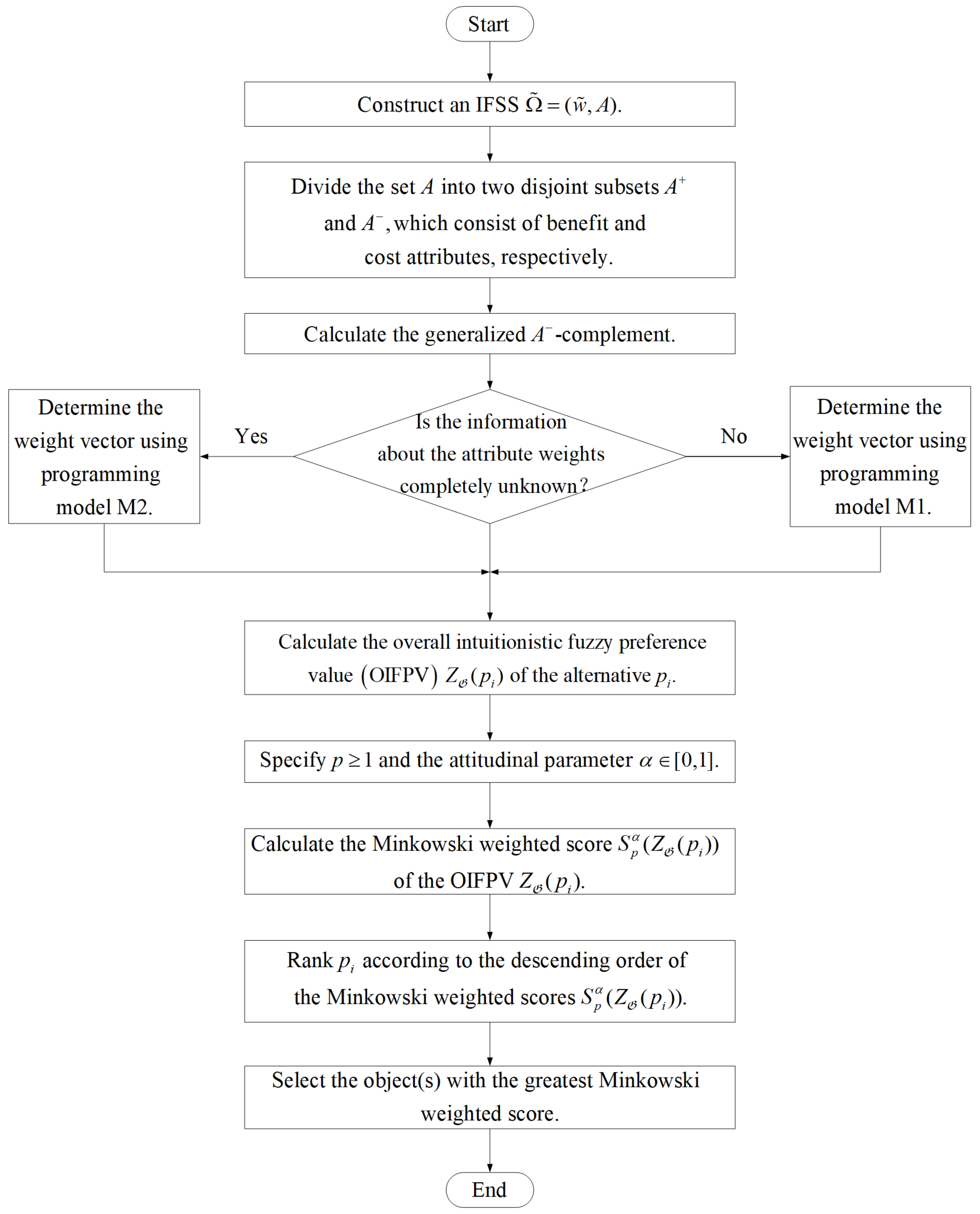
Now, let us solve the above risk investment problem using Algorithm 1 proposed in Section 6. The step-wise description is presented below:

Step 1. Based on the evaluation results adopted from [34], we construct an IFSS $\mathfrak{I}=(\tilde{F},C)$ over $U=\{A_1,A_2,\cdots ,A_5\}$ as shown in

Table 1. Intuitionistic fuzzy soft set $\mathfrak{I}=(\tilde{F},C)$.

U	${\mathit{c}}_1$	${\mathit{c}}_2$	${\mathit{c}}_3$	${\mathit{c}}_4$
$A_1$	$(0.5,0.4)$	$(0.6,0.3)$	$(0.3,0.6)$	$(0.2,0.7)$
$A_2$	$(0.7,0.3)$	$(0.7,0.2)$	$(0.7,0.2)$	$(0.4,0.5)$
$A_3$	$(0.6,0.4)$	$(0.5,0.4)$	$(0.5,0.3)$	$(0.6,0.3)$
$A_4$	$(0.8,0.1)$	$(0.6,0.3)$	$(0.3,0.4)$	$(0.2,0.6)$
$A_5$	$(0.6,0.2)$	$(0.4,0.3)$	$(0.7,0.1)$	$(0.5,0.3)$

.

Step 2. It easy to see that $C^{+}=C$ and $C^{-}=\varnothing$ since $c_1$, $c_2$, $c_3$, and $c_4$ are all benefit attributes.

Step 3. By Definition 6, the generalized $C^{-}$-complement of $\mathfrak{I}$ is:

$$\mathfrak{G}=(\tilde{G},C)={\mathfrak{I}}_{\varnothing }^c=\mathfrak{I},$$

and its approximate function is denoted by:

$$\tilde{G}\left(c_j\right)\left(A_i\right)=(t_{ij}^{\prime },f_{ij}^{\prime }),$$

where $i=1,2,\cdots ,5$ and $j=1,2,\cdots ,4$.

Step 4. In this case, the information about the attribute weights is completely unknown. Accordingly, a single-objective programming model can be established as follows:

$$\begin{array}{cc}\hfill \mathrm{Max}& D\left(W\right)=3.0w_1+2.2w_2+4.8w_3+4.4w_4\hfill \\ \hfill \mathrm{s}.\mathrm{t}.& w_1^2+w_2^2+w_3^2+w_4^2=1\hfill \\ \hfill & w_j\ge 0(j=1,2,3,4).\hfill \end{array}$$

By solving this model, we can get the following optimal solution:

$$W_1^{*}={(0.4000,0.2934,0.6401,0.5867)}^T.$$

After normalization, the obtained weight vector is:

$$W_1={(w_1,w_2,w_3,w_4)}^T={(0.2083,0.1528,0.3333,0.3056)}^T.$$

Step 5. Using the weight vector $W_1$, the OIFPV $Z_{\mathfrak{G}}\left(A_1\right)$ is calculated as follows:

$$Z_{\mathfrak{G}}\left(A_1\right)=\sum _{j=1}^4{w}_j\tilde{G}\left(c_j\right)\left(A_1\right)=(0.3569,0.5431).$$

The OIFPVs of all alternatives $A_i$ ($1\le i\le 5$) can be found in

Table 2. OIFPVs and their corresponding scores.

U	OIFPV: ${\mathit{Z}}_{\mathfrak{G}}\left({\mathit{A}}_{\mathit{i}}\right)$	${\mathit{s}}_2^{0.7}\left({\mathit{Z}}_{\mathfrak{G}}\left({\mathit{A}}_{\mathit{i}}\right)\right)$	$\mathit{s}\left({\mathit{Z}}_{\mathfrak{G}}\left({\mathit{A}}_{\mathit{i}}\right)\right)$
$A_1$	$(0.3569,0.5431)$	0.4294	−0.1862
$A_2$	$(0.6083,0.3125)$	0.6647	0.2958
$A_3$	$(0.5514,0.3361)$	0.6323	0.2153
$A_4$	$(0.4194,0.3834)$	0.5647	0.0360
$A_5$	$(0.5722,0.2125)$	0.7296	0.3597

.

Step 6. Assume that the decision maker specifies $p=2$ and the attitudinal parameter $\alpha =0.7$, respectively.

Step 7. Based on the selected values, we calculate the Euclidean weighted scores $s_2^{0.7}\left(Z_{\mathfrak{G}}\left(A_i\right)\right)$ of the OIFPVs according to Equation (14):

$$s_2^{0.7}\left(Z_{\mathfrak{G}}\left(A_i\right)\right)={\left((1-0.7)t_{Z_{\mathfrak{G}}\left(A_i\right)}^2+0.7{(1-f_{Z_{\mathfrak{G}}\left(A_i\right)})}^2\right)}^{\frac{1}{2}}$$

for $i=1,2,\cdots ,5$. For instance, the Euclidean weighted score $s_2^{0.7}\left(Z_{\mathfrak{G}}\left(A_1\right)\right)$ can be obtained as:

$$s_2^{0.7}\left(Z_{\mathfrak{G}}\left(A_1\right)\right)={\left(0.3t_{Z_{\mathfrak{G}}\left(A_1\right)}^2+0.7{(1-f_{Z_{\mathfrak{G}}\left(A_1\right)})}^2\right)}^{\frac{1}{2}}=0.4294,$$

The other results can be found in Table 2.

Step 8. According to the descending order of the Euclidean weighted score $s_2^{0.7}\left(Z_{\mathfrak{G}}\left(A_i\right)\right)$, the ranking of $A_i$ ($1\le i\le 5$) can be obtained as follows:

$$A_5\succ A_2\succ A_3\succ A_4\succ A_1.$$

Step 9. The optimal decision is to invest in the company $A_5$ since it has the greatest Euclidean weighted score.

In order to verify the effectiveness of the proposed method and its consistency with existing literature, now we make a comparative check against several lexicographic orders introduced in [51] and four other representative methods [34,45,46]. We apply them to the same illustrative example that we have studied above.

According to Definition 15 and the classical scores $s\left(Z_{\mathfrak{G}}\left(A_i\right)\right)$ ($1\le i\le 5$) shown in Table 2, we can obtain the following ranking:

$$A_5\succ A_2\succ A_3\succ A_4\succ A_1.$$

Table 3. Ranking results given by different methods.

Methods	Ranking of the Companies
Algorithm 1 ($p=2,\alpha =0.7$)	$A_5\succ A_2\succ A_3\succ A_4\succ A_1$
SWIFA and ${\le }_{(s,t)}$	$A_5\succ A_2\succ A_3\succ A_4\succ A_1$
SWIFA and ${\le }_{(s,f)}$	$A_5\succ A_2\succ A_3\succ A_4\succ A_1$
SWIFA and ${\le }_{(f,t)}$	$A_5\succ A_2\succ A_3\succ A_4\succ A_1$
SWIFA and ${\le }_{(t,f)}$	$A_2\succ A_5\succ A_3\succ A_4\succ A_1$
Wei’s method [34]	$A_5\succ A_2\succ A_3\succ A_4\succ A_1$
Xia and Xu’s method [45]	$A_5\succ A_2\succ A_3\succ A_4\succ A_1$
Song et al.’s method [46]	$A_5\succ A_2\succ A_3\succ A_4\succ A_1$

summarizes all the ranking results obtained by Algorithm 1, Wei’s method [34], Xia and Xu’s method [45], Song et al.’s method [46], and the lexicographic orders ${\le }_{(s,t)}$, ${\le }_{(s,f)}$, ${\le }_{(f,t)}$, and ${\le }_{(t,f)}$. By comparison, it can be seen that the ranking obtained by Algorithm 1 is only slightly different from the result of the lexicographic order ${\le }_{(t,f)}$. Although the proposed method, Wei’s method [34], Xia and Xu’s method [45], Song et al.’s method [46], and the lexicographic orders ${\le }_{(s,t)}$, ${\le }_{(s,f)}$, and ${\le }_{(f,t)}$ can produce the same ranking of alternatives, the rationales of these approaches is quite different.

Remark 2.

Let us briefly recall some essential facts concerning the approaches that we use for contrast. Wei’s method [34] selects the weight vector w, which maximizes the total weighted deviation value among all options and with respect to all attributes. Xia and Xu’s method [45] determines the optimal weights of attributes based on entropy and cross entropy. According to Xia and Xu’s idea, an attribute with smaller entropy and larger cross entropy should be assigned a larger weight. The design of Song et al.’s similarity measure [46] for IFSs involves Jousselme’s distance measure and the cosine similarity measure between basic probability assignments (BPAs). Their similarity measure can avoid the counter-intuitive outputs by a single evaluation of the similarity measure, and it grants more rationality to the ranking results.

Feng et al. [51] pointed out that lexicographic orders ${\le }_{(s,t)}$, ${\le }_{(s,f)}$, ${\le }_{(f,t)}$, and ${\le }_{(t,f)}$ are not logically equivalent. Therefore, we might observe that they produce different outputs. In our case, notice that the ranking obtained under ${\le }_{(t,f)}$ is different from the other three rankings. It is also worth noting that the rankings derived from ${\le }_{(s,t)}$ and ${\le }_{(s,f)}$ are identical, despite the fact that the scores $Z_{\mathfrak{G}}\left(A_i\right)$$(1\le i\le 5)$ are all different.

This comparison analysis shows that our new approach provides an effective and consistent tool for solving multiple attribute decision-making problems under an intuitionistic fuzzy environment.

7.2. A Supplier Selection Problem

In this subsection, we illustrate Algorithm 1 in the case where the information about the attribute weights is partly known. We revisit a multi-attribute intuitionistic fuzzy group decision-making problem studied in Boran et al. [47]. This reference analyzed a supplier selection problem by means of the TOPSIS method with intuitionistic fuzzy sets. We resort to a modified version of the case study in [47] where the number of alternatives is artificially increased to ten, for the purpose of better understanding Algorithm 1.

Following [47], an automotive company intends to select the most appropriate supplier for one of the key components in its manufacturing process. The selection will be made among ten alternatives in $U=\{s_1,s_2,\cdots s_{10}\}$, which are evaluated based on four criteria. The set consisting of these criteria is denoted by $C=\{e_1,e_2,e_3,e_4\}$, where:

• $e_1$ stands for product quality;
• $e_2$ stands for relationship closeness;
• $e_3$ stands for delivery performance;
• $e_4$ stands for product price.

Now, let us solve the above supplier selection problem using Algorithm 1. The step-wise description is given below:

Step 1. Based on the evaluation results adopted from [47], we construct an IFSS $\mathfrak{I}=(\tilde{F},C)$ over $U=\{s_1,s_2,\cdots ,s_{10}\}$ as shown in

Table 4. Intuitionistic fuzzy soft set $\mathfrak{I}=(\tilde{F},C)$.

U	${\mathit{e}}_1$	${\mathit{e}}_2$	${\mathit{e}}_3$	${\mathit{e}}_4$
$s_1$	$(0.7280,0.1700)$	$(0.6260,0.2720)$	$(0.7800,0.1180)$	$(0.7000,0.2000)$
$s_2$	$(0.5960,0.3020)$	$(0.6050,0.2920)$	$(0.6440,0.2560)$	$(0.5780,0.3210)$
$s_3$	$(0.8490,0.1000)$	$(0.7800,0.1180)$	$(0.7690,0.1700)$	$(0.7690,0.1280)$
$s_4$	$(0.6630,0.2360)$	$(0.5380,0.3610)$	$(0.7460,0.1510)$	$(0.6440,0.2540)$
$s_5$	$(0.5620,0.3370)$	$(0.4620,0.4380)$	$(0.6680,0.2310)$	$(0.5260,0.3740)$
$s_6$	$(0.6620,0.2360)$	$(0.6155,0.2820)$	$(0.7120,0.1870)$	$(0.6390,0.2605)$
$s_7$	$(0.7225,0.2010)$	$(0.6925,0.2050)$	$(0.7065,0.2130)$	$(0.6735,0.2245)$
$s_8$	$(0.7560,0.1680)$	$(0.6590,0.2395)$	$(0.7575,0.1605)$	$(0.7065,0.1910)$
$s_9$	$(0.6125,0.2865)$	$(0.5000,0.3995)$	$(0.7070,0.1910)$	$(0.5850,0.3140)$
$s_{10}$	$(0.6450,0.2535)$	$(0.5440,0.3550)$	$(0.7240,0.1745)$	$(0.6130,0.2870)$

. It should be noted that the evaluations for the alternatives $s_1,s_2,\cdots ,s_5$ are inherited from [47], while the evaluations of the new alternatives $s_6,s_7,\cdots ,s_{10}$ are the simple intuitionistic fuzzy average (SIFA) values of the original values for $s_1,s_2,\cdots ,s_5$, taken by pairs.

For instance, the SIFA of the evaluations of the alternatives $s_1$ and $s_2$ is used as the evaluation result of the artificial alternative $s_6=s_{(1,2)}$. More specifically, by Equation (5), we get:

$$\begin{array}{cc}\hfill \tilde{F}\left(e_1\right)\left(s_{(1,2)}\right)& ={\mathsf{\Xi }}^s\left(\tilde{F}\left(e_1\right)\left(s_1\right),\tilde{F}\left(e_1\right)\left(s_2\right)\right)\hfill \\ \hfill & =(0.6620,0.2360).\hfill \end{array}$$

All other evaluation results can be obtained in a similar fashion. For convenience, we simply write $s_6=s_{(1,2)}$, $s_7=s_{(2,3)}$, $s_8=s_{(3,4)}$, $s_9=s_{(4,5)}$, and $s_{10}=s_{(1,5)}$.

Step 2. Divide the set C into two disjoint subsets $C^{+}$ and $C^{-}$. It is easy to see that $C^{+}=\{e_1,e_2,e_3\}$ and $C^{-}=\left\{e_4\right\}$, since $e_1$, $e_2$ and $e_3$ are benefit attributes, while $e_4$ is a cost attribute.

Step 3. Calculate the generalized $C^{-}$-complement $\mathfrak{G}=(\tilde{G},C)={\mathfrak{I}}_{C^{-}}^c$ of the IFSS $\mathfrak{I}$ according to Definition 6, and the results are shown in

Table 5. Intuitionistic fuzzy soft set $\mathfrak{G}=(\tilde{G},C)={\mathfrak{I}}_{C^{-}}^c$.

U	${\mathit{e}}_1$	${\mathit{e}}_2$	${\mathit{e}}_3$	${\mathit{e}}_4$
$s_1$	$(0.7280,0.1700)$	$(0.6260,0.2720)$	$(0.7800,0.1180)$	$(0.2000,0.7000)$
$s_2$	$(0.5960,0.3020)$	$(0.6050,0.2920)$	$(0.6440,0.2560)$	$(0.3210,0.5780)$
$s_3$	$(0.8490,0.1000)$	$(0.7800,0.1180)$	$(0.7690,0.1700)$	$(0.1280,0.7690)$
$s_4$	$(0.6630,0.2360)$	$(0.5380,0.3610)$	$(0.7460,0.1510)$	$(0.2540,0.6440)$
$s_5$	$(0.5620,0.3370)$	$(0.4620,0.4380)$	$(0.6680,0.2310)$	$(0.3740,0.5260)$
$s_6$	$(0.6620,0.2360)$	$(0.6155,0.2820)$	$(0.7120,0.1870)$	$(0.2605,0.6390)$
$s_7$	$(0.7225,0.2010)$	$(0.6925,0.2050)$	$(0.7065,0.2130)$	$(0.2245,0.6735)$
$s_8$	$(0.7560,0.1680)$	$(0.6590,0.2395)$	$(0.7575,0.1605)$	$(0.1910,0.7065)$
$s_9$	$(0.6125,0.2865)$	$(0.5000,0.3995)$	$(0.7070,0.1910)$	$(0.3140,0.5850)$
$s_{10}$	$(0.6450,0.2535)$	$(0.5440,0.3550)$	$(0.7240,0.1745)$	$(0.2870,0.6130)$

. For convenience, the approximate function of $\mathfrak{G}$ is denoted by:

$$\tilde{G}\left(e_j\right)\left(s_i\right)=(t_{ij}^{\prime },f_{ij}^{\prime }),$$

where $i=1,2,\cdots ,10$ and $j=1,2,\cdots ,4$.

Step 4. In this case, the information about the attribute weights is partly known. Accordingly, a single-objective programming model can be established as follows:

$$\begin{array}{cc}\hfill \mathrm{Max}& D\left(W\right)=8.325w_1+10.179w_2+4.455w_3+7.736w_4\hfill \\ \hfill \mathrm{s}.\mathrm{t}.& 0.25\le w_1\le 0.30\hfill \\ \hfill & 0.26\le w_2\le 0.31\hfill \\ \hfill & 0.23\le w_3\le 0.28\hfill \\ \hfill & 0.08\le w_4\le 0.14\hfill \\ \hfill & w_1+w_2+w_3+w_4=1\hfill \\ \hfill & w_j\ge 0(j=1,2,3,4).\hfill \end{array}$$

By solving this model, we can get the following normalized optimal weight vector:

$$W_2={(w_1,w_2,w_3,w_4)}^T={(0.30,0.31,0.25,0.14)}^T.$$

Step 5. Using the weight vector $W_2$, the OIFPVs of all alternatives $s_i(1\le i\le 10)$ can be calculated, and the results are presented in

Table 6. OIFPVs and their scores with $p=3$ and $\alpha =0.5,0.2,0.8$.

U	${\mathit{Z}}_{\mathfrak{G}}\left({\mathit{s}}_{\mathit{i}}\right)$	${\mathit{s}}_3^{0.5}\left({\mathit{Z}}_{\mathfrak{G}}\left({\mathit{s}}_{\mathit{i}}\right)\right)$	${\mathit{s}}_3^{0.2}\left({\mathit{Z}}_{\mathfrak{G}}\left({\mathit{s}}_{\mathit{i}}\right)\right)$	${\mathit{s}}_3^{0.8}\left({\mathit{Z}}_{\mathfrak{G}}\left({\mathit{s}}_{\mathit{i}}\right)\right)$	$\mathit{s}\left({\mathit{Z}}_{\mathfrak{G}}\left({\mathit{s}}_{\mathit{i}}\right)\right)$
$s_1$	$(0.6355,0.2628)$	0.6901	0.6584	0.7191	0.3726
$s_2$	$(0.5723,0.3260)$	0.6272	0.5955	0.6561	0.2462
$s_3$	$(0.7067,0.2167)$	0.7469	0.7233	0.7691	0.4899
$s_4$	$(0.5877,0.3106)$	0.6426	0.6109	0.6714	0.2771
$s_5$	$(0.5312,0.3683)$	0.5858	0.5543	0.6142	0.1629
$s_6$	$(0.6039,0.2944)$	0.6586	0.6269	0.6876	0.3094
$s_7$	$(0.6395,0.2714)$	0.6869	0.6593	0.7125	0.3681
$s_8$	$(0.6472,0.2637)$	0.6946	0.6670	0.7202	0.3835
$s_9$	$(0.5595,0.3394)$	0.6142	0.5826	0.6428	0.2200
$s_{10}$	$(0.5833,0.3155)$	0.6379	0.6063	0.6666	0.2678

.

Step 6. Assume that the decision maker specifies $p=3$ and the attitudinal parameter $\alpha =0.5$, respectively. As mentioned in Remark 1, the Minkowski weighted score function is reduced to the Minkowski score function when the attitudinal parameter $\alpha =0.5$, representing the decision maker’s neutral attitude.

Step 7. Based on the selected values, we calculate the Minkowski weighted scores $s_3^{0.5}\left(Z_{\mathfrak{G}}\left(s_i\right)\right)$ of the OIFPVs according to Equation (10):

$$s_3^{0.5}\left(Z_{\mathfrak{G}}\left(s_i\right)\right)=s_3\left(Z_{\mathfrak{G}}\left(s_i\right)\right)={\left(\frac{t_{Z_{\mathfrak{G}}\left(s_i\right)}^3+{(1-f_{Z_{\mathfrak{G}}\left(s_i\right)})}^3}{2}\right)}^{\frac{1}{3}}$$

for $i=1,2,\cdots ,10$. For instance, the Minkowski weighted score $s_3^{0.5}\left(Z_{\mathfrak{G}}\left(s_1\right)\right)$ is:

$$s_3^{0.5}\left(Z_{\mathfrak{G}}\left(s_1\right)\right)={\left(\frac{t_{Z_{\mathfrak{G}}\left(s_1\right)}^3+{(1-f_{Z_{\mathfrak{G}}\left(s_1\right)})}^3}{2}\right)}^{\frac{1}{3}}={\left(\frac{{0.6355}^3+{(1-0.2628)}^3}{2}\right)}^{\frac{1}{3}}=0.6901.$$

To make a thorough comparison, we also consider two other cases in which $\alpha =0.2$ and $\alpha =0.8$, representing the decision maker’s negative and positive attitudes, respectively. Table 6 gives all the OIFPVs and their Minkowski weighted scores with $p=3$ and various choices of the attitudinal parameter $\alpha$.

Step 8. The ranking of $s_i$ ($i=1,2,\cdots ,10$) based on the descending order of the Minkowski weighted scores $s_3^{0.5}\left(Z_{\mathfrak{G}}\left(s_i\right)\right)$ can be obtained as follows:

$$s_3\succ s_8\succ s_1\succ s_7\succ s_6\succ s_4\succ s_{10}\succ s_2\succ s_9\succ s_5.$$

Step 9. The optimal decision is to select the supplier $s_3$ since it has the greatest Minkowski weighted score.

The analysis above presumes a neutral attitude, i.e., $\alpha =0.5$. In order to visualize the influence of the attitudinal parameter on the final ranking, let us now see what conclusion we draw when we keep $p=3$ and rank the alternatives with two other choices of the attitudinal parameter $\alpha$. Table 6 gives the Minkowski weighted scores $s_3^{0.2}\left(Z_{\mathfrak{G}}\left(s_i\right)\right)$ and $s_3^{0.8}\left(Z_{\mathfrak{G}}\left(s_i\right)\right)$ of the OIFPVs $Z_{\mathfrak{G}}\left(s_i\right)$$(1\le i\le 10)$. They correspond to a negative attitudinal parameter $\alpha =0.2$ and a positive attitude that we associate with $\alpha =0.8$, respectively. It is interesting to observe that the rankings are almost identical to the ranking under a neutral attitude. This indicates that Algorithm 1 is to some extent robust with respect to the choice of the attitudinal parameter.

In addition, Boran et al. introduced the TOPSIS method based on intuitionistic fuzzy sets in [47], which can be used for ranking IFVs as well. To further verify the rationality of the proposed methods, we proceed to compare the ranking that arises from the weight vector $W_2$ obtained by Algorithm 1, the intuitionistic fuzzy TOPSIS method, and various lexicographic orders. Similarly, the ranking results of lexicographic orders can be obtained based on the classical scores $s\left(Z_{\mathfrak{G}}\left(s_i\right)\right)(i=1,2,\cdots ,10)$ listed in Table 6.

The attribute weight vector in [47] is an IFV representation based on the opinions of experts, and it is different from the expression of $W_2$. Therefore, the construction of the aggregate weighted intuitionistic fuzzy decision matrix in Step 4 of the intuitionistic fuzzy TOPSIS method in [47] must be changed. Assume that $\mu$ is the fuzzy set in C such that $\mu \left(e_j\right)=w_j$ ($1\le j\le 4$). Then, the weighted IFSS can easily be obtained by calculating the scalar product $\mathfrak{R}=\mu ⨀\mathfrak{G}=(\tilde{R},C)$ of the IFSS $\mathfrak{G}$ and the fuzzy set $\mu$. For instance, by Definition 7 and Equation (2), we have:

$$\begin{array}{cc}\hfill \tilde{R}\left(e_1\right)\left(s_1\right)& =\left(1-{\left(1-t_{\tilde{G}\left(e_1\right)\left(s_1\right)}\right)}^{\mu \left(e_1\right)},f_{\tilde{G}\left(e_1\right)\left(s_1\right)}^{\mu \left(e_1\right)}\right)\hfill \\ & =\left(1-{\left(1-t_{\tilde{G}\left(e_1\right)\left(s_1\right)}\right)}^{w_1},f_{\tilde{G}\left(e_1\right)\left(s_1\right)}^{w_1}\right)\hfill \\ & =\left(1-{\left(1-0.7280\right)}^{0.30},{0.1700}^{0.30}\right)\hfill \\ & =(0.3233,0.5876).\hfill \end{array}$$

The weighted IFSS that arises is shown in

Table 7. Weighted IFSS $\mathfrak{R}=\mu ⨀\mathfrak{G}=(\tilde{R},C)$.

U	${\mathit{e}}_1$	${\mathit{e}}_2$	${\mathit{e}}_3$	${\mathit{e}}_4$
$s_1$	$(0.3233,0.5876)$	$(0.2627,0.6679)$	$(0.3151,0.5860)$	$(0.1551,0.7982)$
$s_2$	$(0.2380,0.6982)$	$(0.2502,0.6827)$	$(0.2275,0.7113)$	$(0.1137,0.8529)$
$s_3$	$(0.4328,0.5011)$	$(0.3746,0.5155)$	$(0.3067,0.6421)$	$(0.1854,0.7499)$
$s_4$	$(0.2784,0.6484)$	$(0.2128,0.7291)$	$(0.2900,0.6233)$	$(0.1346,0.8254)$
$s_5$	$(0.2193,0.7215)$	$(0.1748,0.7742)$	$(0.2409,0.6932)$	$(0.0992,0.8713)$
$s_6$	$(0.2777,0.6484)$	$(0.2564,0.6754)$	$(0.2674,0.6575)$	$(0.1329,0.8283)$
$s_7$	$(0.3192,0.6179)$	$(0.3062,0.6118)$	$(0.2639,0.6793)$	$(0.1450,0.8112)$
$s_8$	$(0.3450,0.5855)$	$(0.2836,0.6420)$	$(0.2982,0.6329)$	$(0.1577,0.7931)$
$s_9$	$(0.2475,0.6872)$	$(0.1933,0.7524)$	$(0.2642,0.6610)$	$(0.1158,0.8502)$
$s_{10}$	$(0.2670,0.6625)$	$(0.2160,0.7253)$	$(0.2751,0.6463)$	$(0.1244,0.8396)$

.

By performing the rest of the steps of the intuitionistic fuzzy TOPSIS method in [47], we get

Table 8. Separation measures and the relative closeness coefficients.

U	${\mathit{S}}_{\mathit{i}}^{+}$	${\mathit{S}}_{\mathit{i}}^{-}$	${\mathit{C}}_{\mathit{i}}^{*}$
$s_1$	0.0892	0.0964	0.5195
$s_2$	0.1342	0.0619	0.3158
$s_3$	0.0564	0.1628	0.7428
$s_4$	0.1238	0.0635	0.3389
$s_5$	0.1651	0.0533	0.2440
$s_6$	0.1093	0.0694	0.3884
$s_7$	0.0848	0.0949	0.5282
$s_8$	0.0800	0.0983	0.5515
$s_9$	0.1444	0.0519	0.2645
$s_{10}$	0.1272	0.0593	0.3178

, which consists of the Euclidean distance $S_i^{+}(i=1,2,\cdots ,10)$ between each object and the positive ideal solution, the Euclidean distance $S_i^{-}(i=1,2,\cdots ,10)$ between each object and the negative ideal solution, and the relative closeness coefficient $C_i^{*}(i=1,2,\cdots ,10)$. According to the intuitionistic fuzzy TOPSIS method, we can obtain the ranking results based on the descending order of the relative closeness coefficient $C_i^{*}$ as shown in

Table 9. Ranking results based on different methods.

Methods	Ranking of the Suppliers
Boran et al.’s method [47]	$s_3\succ s_8\succ s_7\succ s_1\succ s_6\succ s_4\succ s_{10}\succ s_2\succ s_9\succ s_5$
Algorithm 1 ($p=3,\alpha =0.2)$	$s_3\succ s_8\succ s_7\succ s_1\succ s_6\succ s_4\succ s_{10}\succ s_2\succ s_9\succ s_5$
Algorithm 1 ($p=3,\alpha =0.5$)	$s_3\succ s_8\succ s_1\succ s_7\succ s_6\succ s_4\succ s_{10}\succ s_2\succ s_9\succ s_5$
Algorithm 1 ($p=3,\alpha =0.8$)	$s_3\succ s_8\succ s_1\succ s_7\succ s_6\succ s_4\succ s_{10}\succ s_2\succ s_9\succ s_5$
SWIFA and ${\le }_{(s,t)}$	$s_3\succ s_8\succ s_1\succ s_7\succ s_6\succ s_4\succ s_{10}\succ s_2\succ s_9\succ s_5$
SWIFA and ${\le }_{(s,f)}$	$s_3\succ s_8\succ s_1\succ s_7\succ s_6\succ s_4\succ s_{10}\succ s_2\succ s_9\succ s_5$
SWIFA and ${\le }_{(f,t)}$	$s_3\succ s_1\succ s_8\succ s_7\succ s_6\succ s_4\succ s_{10}\succ s_2\succ s_9\succ s_5$
SWIFA and ${\le }_{(t,f)}$	$s_3\succ s_8\succ s_7\succ s_1\succ s_6\succ s_4\succ s_{10}\succ s_2\succ s_9\succ s_5$

.

Table 9 summarizes all the ranking results obtained by Algorithm 1 (with three different attitudinal parameters $\alpha$), the intuitionistic fuzzy TOPSIS method [47], and the lexicographic orders ${\le }_{(s,t)}$, ${\le }_{(s,f)}$, ${\le }_{(f,t)}$, and ${\le }_{(t,f)}$. By comparison, it can be seen that the ranking obtained by Algorithm 1 with the pessimistic attitude is only slightly different from those obtained with either the neutral or optimistic attitude. Algorithm 1 with either the neutral or optimistic attitude and the lexicographic orders ${\le }_{(s,t)}$, ${\le }_{(s,f)}$ produce the same results. The ranking given by Algorithm 1 with the pessimistic attitude coincides with the results of the lexicographic orders ${\le }_{(t,f)}$ and the intuitionistic fuzzy TOPSIS method. Whatever the choice, the best supplier is $s_3$, and the worst supplier is $s_5$. Thus, this numerical example concerning supplier selection further illustrates that the method proposed in this study is feasible for solving multiple attribute decision-making problems in real-life environments.

Remark 3.

Let us briefly highlight several key points with regard to the above discussion. Note first that the set of alternatives is expanded from the original set [47] consisting of five alternatives to a new set containing ten alternatives. All the evaluation results of these alternatives are shown in Table 4. It should be noted that the evaluation results of the alternatives $s_i$ ($i=1,2,\cdots ,5$) are inherited directly from [47]. In contrast, the alternatives $s_i$ ($i=6,7,\cdots ,10$) in Table 4 are artificial ones, and the evaluation results of them are obtained by computing the SIFA values of the IFVs associated with $s_1,s_2,\cdots ,s_5$ in a pairwise manner. Note also that the obtained artificial alternatives $s_6,s_7,\cdots ,s_{10}$ provide an additional way to verify the rationality of Algorithm 1. In fact, we can see from Table 9 that each artificial alternative lies between the two original alternatives that are used to produce it. For instance, $s_6=s_{(1,2)}$ lies between $s_1$ and $s_2$ in all the ranking results. This is due to the fact that we obtain the evaluation results of $s_6$ by simply averaging the corresponding results of $s_1$ and $s_2$. Finally, the ranking results in Table 9 with $\alpha =0.2$, $\alpha =0.5$, and $\alpha =0.8$ show that the selection of different attitudinal parameters may affect the final ranking results. However, to a certain extent, Algorithm 1 is robust with respect to the choice of the attitudinal parameter as well.

8. Conclusions

Based on the geometric intuition that a better score should be assigned to an intuitionistic fuzzy value farther from the negative ideal intuitionistic fuzzy value ${\alpha }_{*}=(0,1)$, Minkowski score functions of intuitionistic fuzzy values were proposed for comparing intuitionistic fuzzy values in the complete lattice $L^{*}$. By taking into account an attitudinal parameter, we also presented the concept of Minkowski weighted score functions, which enabled us to describe the decision makers’ subjective attitudes as well. We investigated some basic properties of Minkowski (weighted) score functions and developed a new algorithm for solving multiple attribute decision-making problems based on intuitionistic fuzzy soft sets. Based on two numerical examples concerning risk investment and supplier selection, a brief comparative analysis was made between the newly proposed algorithm and existing alternatives in the literature. It was shown that our method was feasible for solving intuitionistic fuzzy soft set based decision-making problems in real-world scenarios.

Our fundamental tool (Minkowski weighted score function) can be used in the future for the efficient aggregation of infinite chains of intuitionistic fuzzy sets [56]. This line of research concerns decisions in a temporal setting, possibly with an infinite horizon. The breadth of the theory of the aggregation of infinite streams of numbers was discussed in [57] and the references therein.

References

1. Ishizaka, A.; Nemery, P. Multi-Criteria Decision Analysis: Methods and Software; Wiley: Chichester, UK, 2013. [Google Scholar]
2. Pamučar, D.S.; Savin, L.M. Multiple-criteria model for optimal off-road vehicle selection for passenger transportation: BWM-COPRAS model. Vojnoteh. Glas. 2020, 68, 28–64. [Google Scholar] [CrossRef]
3. Xu, Z.S. Uncertain Multi-Attribute Decision Making; Tsinghua University Press: Beijing, China, 2004. [Google Scholar]
4. Zadeh, L.A. Fuzzy sets. Inf. Control 1965, 8, 338–353. [Google Scholar] [CrossRef] [Green Version]
5. Rahman, S. On cuts of Atanassov’s intuitionistic fuzzy sets with respect to fuzzy connectives. Inf. Sci. 2016, 340, 262–278. [Google Scholar] [CrossRef]
6. Atanassov, K.T. Intuitionistic fuzzy sets. In Intuitionistic Fuzzy Sets; Physica: Heidelberg, Germany, 1986; Volume 20, pp. 87–96. [Google Scholar]
7. Xu, Z.S.; Yager, R.R. Some geometric aggregation operators based on intuitionistic fuzzy sets. Int. J. Gen. Syst. 2006, 35, 417–433. [Google Scholar] [CrossRef]
8. Yager, R.R. Multicriteria decision making with ordinal/linguistic intuitionistic fuzzy sets for mobile apps. IEEE Trans. Fuzzy Syst. 2016, 24, 590–599. [Google Scholar] [CrossRef]
9. Molodtsov, D.A. Soft set theory-first results. Comput. Math. Appl. 1999, 37, 19–31. [Google Scholar] [CrossRef] [Green Version]
10. Feng, F.; Cho, J.; Pedrycz, W.; Fujita, H.; Herawan, T. Soft set based association rule mining. Knowl. Based Syst. 2016, 111, 268–282. [Google Scholar] [CrossRef]
11. Ali, M.I.; Feng, F.; Liu, X.Y.; Min, W.K.; Shabir, M. On some new operations in soft set theory. Comput. Math. Appl. 2009, 57, 1547–1553. [Google Scholar] [CrossRef] [Green Version]
12. Ali, M.I.; Shabir, M.; Naz, M. Algebraic structures of soft sets associated with new operations. Comput. Math. Appl. 2011, 61, 2647–2654. [Google Scholar] [CrossRef] [Green Version]
13. Ali, M.I.; Shabir, M. Logic connectives for soft sets and fuzzy soft sets. IEEE Trans. Fuzzy Syst. 2014, 22, 1431–1442. [Google Scholar] [CrossRef]
14. Feng, F.; Li, Y.M. Soft subsets and soft product operations. Inf. Sci. 2013, 232, 44–57. [Google Scholar] [CrossRef]
15. Jun, Y.B.; Lee, K.J.; Khan, A. Soft ordered semigroups. Math. Log. Q. 2010, 56, 42–50. [Google Scholar] [CrossRef]
16. Jun, Y.B.; Park, C.H. Applications of soft sets in ideal theory of BCK/BCI-algebras. Inf. Sci. 2008, 178, 2466–2475. [Google Scholar] [CrossRef]
17. Jun, Y.B. Soft BCK/BCI-algebras. Comput. Math. Appl. 2008, 56, 1408–1413. [Google Scholar] [CrossRef] [Green Version]
18. Maji, P.K.; Biswas, R.; Roy, A.R. Fuzzy soft sets. J. Fuzzy Math. 2001, 9, 589–602. [Google Scholar]
19. Das, S.; Kar, S. The hesitant fuzzy soft set and its application in decision-making. In Facets of Uncertainties and Applications. Springer Proceedings in Mathematics & Statistics; Chakraborty, M.K., Skowron, A., Maiti, M., Kar, S., Eds.; Springer: New Delhi, India, 2015; Volume 125. [Google Scholar]
20. Das, S.; Malakar, D.; Kar, S.; Pal, T. Correlation measure of hesitant fuzzy soft sets and their application in decision making. Neural Comput. Appl. 2019, 31, 1023–1039. [Google Scholar] [CrossRef]
21. Fatimah, F.; Rosadi, D.; Hakim, R.B.F.; Alcantud, J.C.R. N-soft sets and their decision making algorithms. Soft Comput. 2018, 22, 3829–3842. [Google Scholar] [CrossRef]
22. Alcantud, J.C.R.; Feng, F.; Yager, R.R. An N-soft set approach to rough sets. IEEE Trans. Fuzzy Syst. 2019. [Google Scholar] [CrossRef]
23. Akram, M.; Adeel, A.; Alcantud, J.C.R. Group decision-making methods based on hesitant N-soft sets. Expert Syst. Appl. 2019, 115, 95–105. [Google Scholar] [CrossRef]
24. Akram, M.; Adeel, A.; Alcantud, J.C.R. Fuzzy N-soft sets: A novel model with applications. J. Intell. Fuzzy Syst. 2018, 35, 4757–4771. [Google Scholar] [CrossRef]
25. Maji, P.K.; Biswas, R.; Roy, A.R. Intuitionistic fuzzy soft sets. J. Fuzzy Math. 2001, 9, 677–692. [Google Scholar]
26. Ali, M.I.; Feng, F.; Mahmood, T.; Mahmood, I.; Faizan, H. A graphical method for ranking Atanassov’s intuitionistic fuzzy values using the uncertainty index and entropy. Int. J. Intell. Syst. 2019, 34, 2692–2712. [Google Scholar] [CrossRef]
27. Feng, F.; Xu, Z.; Fujita, H.; Liang, M. Enhancing PROMETHEE method with intuitionistic fuzzy soft sets. Int. J. Intell. Syst. 2020, 35, 1071–1104. [Google Scholar] [CrossRef]
28. Agarwal, M.; Biswas, K.K.; Hanmandlu, M. Generalized intuitionistic fuzzy soft sets with applications in decision-making. Appl. Soft Comput. 2013, 13, 3552–3566. [Google Scholar] [CrossRef]
29. Feng, F.; Fujita, H.; Ali, M.I.; Yager, R.R.; Liu, X. Another view on generalized intuitionistic fuzzy soft sets and related multiattribute decision making methods. IEEE Trans. Fuzzy Syst. 2019, 27, 474–488. [Google Scholar] [CrossRef]
30. Peng, X.D.; Yang, Y.; Song, J.P. Pythagoren fuzzy soft set and its application. Comput. Eng. 2015, 41, 224–229. [Google Scholar]
31. Athira, T.M.; John, S.J.; Garg, H. A novel entropy measure of Pythagorean fuzzy soft sets. AIMS Math. 2019, 5, 1050–1061. [Google Scholar] [CrossRef]
32. Dey, A.; Senapati, T.; Pal, M.; Chen, G.Y. A novel approach to hesitant multi-fuzzy soft set based decision-making. AIMS Math. 2020, 5, 1985–2008. [Google Scholar] [CrossRef]
33. Das, S.; Kar, M.B.; Kar, S. Group multi-criteria decision making using intuitionistic multi-fuzzy sets. J. Uncertain. Anal. Appl. 2013, 1, 10. [Google Scholar] [CrossRef] [Green Version]
34. Wei, G.W. Maximizing deviation method for multiple attribute decision making in intuitionistic fuzzy setting. Knowl. Based Syst. 2008, 21, 833–836. [Google Scholar] [CrossRef]
35. Liu, X.; Kim, H.S.; Feng, F.; Alcantud, J.C.R. Centroid transformations of intuitionistic fuzzy values based on aggregation operators. Mathematics 2018, 6, 215. [Google Scholar] [CrossRef] [Green Version]
36. Chen, S.M.; Tan, J.M. Handling multicriteria fuzzy decision-making problems based on vague set theory. Fuzzy Sets Syst. 1994, 67, 163–172. [Google Scholar] [CrossRef]
37. Hong, D.H.; Choi, C.H. Multi-criteria fuzzy decision-making problems based on vague set theory. Fuzzy Sets Syst. 2000, 114, 103–113. [Google Scholar] [CrossRef]
38. Yu, X.; Xu, Z.; Liu, S.; Chen, Q. On ranking of intuitionistic fuzzy values based on dominance relations. Int. J. Uncertain. Fuzziness Knowl. Based Syst. 2014, 22, 315–335. [Google Scholar] [CrossRef]
39. Garg, H.; Arora, R. TOPSIS method based on correlation coefficient for solving decision-making problems with intuitionistic fuzzy soft set information. AIMS Math. 2020, 5, 2944–2966. [Google Scholar] [CrossRef]
40. Szmidt, E.; Kacprzyk, J. Amount of infornation and its reliability in the ranking of Atanassov’s intuitionistic fuzzy alternatives. In Recent Advances in Decision Making; Series Studies in Computational Intelligence; Springer: Berlin/Heidelberg, Germany, 2009; pp. 7–19. [Google Scholar]
41. Guo, K. Amount of information and attitudinal-based method for ranking Atanassov’s intuitionistic fuzzy values. IEEE Trans. Fuzzy Syst. 2014, 22, 177–188. [Google Scholar] [CrossRef]
42. Zhang, X.; Xu, Z. A new method for ranking intuitionistic fuzzy values and its application in multi-attribute decision making. Fuzzy Optim. Decis. Mak. 2012, 11, 135–146. [Google Scholar] [CrossRef]
43. Wang, W.; Xin, X. Distance measure between intuitionistic fuzzy sets. Pattern Recognit. Lett. 2005, 26, 2063–2069. [Google Scholar] [CrossRef]
44. Xing, Z.; Xiong, W.; Liu, H. A Euclidean approach for ranking intuitionistic fuzzy values. IEEE Trans. Fuzzy Syst. 2018, 26, 353–365. [Google Scholar] [CrossRef]
45. Xia, M.M.; Xu, Z.S. Entropy/cross entropy-based group decision making under intuitionistic fuzzy environment. Inf. Fusion 2012, 13, 31–47. [Google Scholar] [CrossRef]
46. Song, Y.F.; Wang, X.D.; Lei, L.; Quan, W.; Huang, W.L. An evidential view of similarity measure for Atanassov’s intuitionistic fuzzy sets. J. Intell. Fuzzy Syst. 2016, 31, 1653–1668. [Google Scholar] [CrossRef]
47. Boran, F.E.; Genc, S.; Kurt, M.; Akay, D. A multi-criteria intuitionistic fuzzy group decision making for supplier selection with TOPSIS method. Expert Syst. Appl. 2009, 36, 11363–11368. [Google Scholar] [CrossRef]
48. Wang, G.J.; He, Y.Y. Intuitionistic fuzzy sets and L-fuzzy sets. Fuzzy Sets Syst. 2000, 10, 271–274. [Google Scholar] [CrossRef]
49. Deschrijver, G.; Kerre, E.E. On the relationship between some extensions of fuzzy set theory. Fuzzy Sets Syst. 2003, 133, 227–235. [Google Scholar] [CrossRef]
50. Alcantud, J.C.R.; Cruz-Rambaud, S.; Muñoz Torrecillas, M.J. Valuation fuzzy soft sets: A flexible fuzzy soft set based decision making procedure for the valuation of assets. Symmetry 2017, 9, 253. [Google Scholar] [CrossRef] [Green Version]
51. Feng, F.; Liang, M.; Fujita, H.; Yager, R.R.; Liu, X. Lexicographic orders of intuitionistic fuzzy values and their relationships. Mathematics 2019, 7, 166. [Google Scholar] [CrossRef] [Green Version]
52. Xu, Z.S.; Yager, R.R. Intuitionistic and interval-valued intutionistic fuzzy preference relations and their measures of similarity for the evaluation of agreement within a group. Fuzzy Optim. Decis. Mak. 2009, 8, 123–139. [Google Scholar] [CrossRef]
53. Xu, Z.S. Models for multiple attribute decision-making with intuitionistic fuzzy information. Int. J. Uncertain. Fuzziness Knowl. Based Syst. 2007, 15, 285–297. [Google Scholar] [CrossRef]
54. Herrera, F.; Herrera-Viedma, E. Linguistic decision analysis: Steps for solving decision problems under linguistic information. Fuzzy Sets Syst. 2000, 115, 67–82. [Google Scholar] [CrossRef]
55. Chen, L.H.; Tu, C.C. Dual bipolar measures of Atanassov’s intuitionistic fuzzy sets. IEEE Trans. Fuzzy Syst. 2014, 22, 966–982. [Google Scholar] [CrossRef]
56. Alcantud, J.C.R.; Khameneh, A.Z.; Kilicman, A. Aggregation of infinite chains of intuitionistic fuzzy sets and their application to choices with temporal intuitionistic fuzzy information. Inf. Sci. 2020, 514, 106–117. [Google Scholar] [CrossRef]
57. Alcantud, J.C.R.; García-Sanz, M.D. Evaluations of infinite utility streams: Pareto efficient and egalitarian axiomatics. Metroeconomica 2013, 64, 432–447. [Google Scholar] [CrossRef] [Green Version]
Figure 1. Workflow and framework of this study. IFSS, intuitionistic fuzzy soft set; MADM, multiple attribute decision making (MADM); SWIFA, simply weighted intuitionistic fuzzy averaging.
Mathematics 08 01143 g001
Figure 2. Flowchart of the proposed algorithm for intuitionistic fuzzy MADM.
Mathematics 08 01143 g002