Tube-Based Taut String Algorithms for Total Variation Regularization

Abstract

Removing noise from signals using total variation regularization is a challenging signal processing problem arising in many practical applications. The taut string method is one of the most efficient approaches for solving the 1D TV regularization problem. In this paper we propose a geometric description of the linearized taut string method. This geometric description leads to the notion of the “tube”. We propose three tube-based taut string algorithms for total variation regularization. Different weight functionals can be used in the 1D TV regularization that lead to different types of tubes. We consider uniform, vertically nonuniform, vertically and horizontally nonuniform tubes. The proposed geometric approach is used to speed-up TV regularization processing by dividing the tubes into subtubes and using parallel processing. We introduce the concept of a relatively convex tube and describe the relationship between the geometric characteristics of tubes and exact solutions to the TV regularization. The properties of exact solutions can also be used to design efficient algorithms for solving the TV regularization problem. The performance of the proposed algorithms is discussed and illustrated by computer simulation.

1. Introduction

The total variation regularization (TV regularization) is one of the most efficient techniques of signal denoising. The TV denoising problem has received great attention in the communities of signal and image processing, inverse and ill-posed problems, statistical regression analysis, optimization theory, etc. [1,2]. TV regularization techniques are also used in image recovery applications, such as deblurring and space-variant restoration [3,4,5,6,7,8,9]. TV regularization looks for a denoised signal u from the noisy function $u_0$, implicitly defined as a solution to minimizing TV, but without much bias towards a sharp or smooth solution. A better understanding of TV regularization is necessary for a more rigorous mathematical justification for the use of TV minimization in image processing or other regularization applications [10,11,12,13]. The description of exact solutions to the TV regularization problem is important for understanding how TV regularization affects functions. Chambolle and Pock [14] described the state-of-the-art methods of TV regularization. 1D TV regularization algorithms are widely used to solve 2D and multidimensional anisotropic TV regularization problems.

Let $J\left(u\right)$ be the following functional:

$$J\left(u\right)=\frac{1}{2}{\parallel u-u_0\parallel }^2+\lambda TV\left(u\right),$$

(1)

where $\parallel .\parallel$ is the $L^2$ norm and functions u, $u_0$ belong to the class of bounded variation functions $BV(\Omega )$ on a set $\Omega \subset {\mathbf{R}}^2$. The expression $\frac{1}{2}{\parallel u-u_0\parallel }^2$ is called the fidelity term and the expression $\lambda TV\left(u\right)$ is called the regularization term. The definition of total variation $TV\left(u\right)$ of the function u is borrowed from [1]. Here $u_0$ is the observed signal (noisy function) distorted by additive noise n,

$$u_0=v+n,$$

(2)

where v is an original undistorted function. Let us consider the following variational problem:

$$u_{*}=arg\underset{u\in BV(\Omega )}{min}J\left(u\right).$$

(3)

The observed signal $u_0$ and the regularization parameter $\lambda$ determine the sharpness or smoothness of the restored signal. Larger values of the parameter $\lambda$ lead to a greater regularization and less goodness of fitting u to the noisy signal $u_0$.

Davies and Kovac considered the problem (3) as non-parametric regression and introduced the taut string method for discrete functions [15]. The complexity of the algorithm is $O\left(N\right)$ for any 1D discrete function where N is the number of discrete function samples. Other algorithms [16,17] have also been proposed to solve the 1D TV variational problem. Their complexity is equal to $O\left(N\right)$ for an arbitrary descrete function. A direct 1D TV regularization method based on the use of a subgradient was suggested [17].

Condat described a direct fast algorithm for searching the exact solutions to the 1D TV regularization problem for discrete functions [18]. The system of equations describing an extremal function there was derived by solving the dual variational problem. In general, the complexity of the algorithm is $O\left(N^2\right)$; however, for a wide class of common functions the complexity is $O\left(N\right)$ [18]. Recently, the Condat method was described using the linearized taut string method and its geometric interpretation is given [19,20].

The geometrical interpretation leads to the concept of tube. The term tube means a closed piecewise linear curve (without self-intersections) in ${\mathbf{R}}^2$, which is defined by observed function $u_0$. The curve divides ${\mathbf{R}}^2$ onto external and internal parts. The solution of the variational problem (3) can be described by a piecewise linear curve that belongs to the internal part relative to the tube.

The standard 1D TV regularization problem corresponds to the uniform tubes, i.e., tubes with a fixed horizontal step and a fixed width. The 1D TV problem with the weight coefficients for the regularization term leads to vertically nonuniform tubes [19,20]. The 1D TV regularization is reduced to the problem of constructing of a taut string in a tube. The same geometrical interpretation was proposed independently and partially earlier [21,22,23,24]. The proposed paper is a significantly extended version of the papers. The 1D TV regularization with a functional containing the weight coefficients in the fidelity term leads to horizontally nonuniform tubes. Note that nonuniform tubes naturally arise in 2D isotropic TV regularization for piecewise constant radially symmetric functions [25].

Condat [18] solved the 1D TV regularization problem by using the Karush–Kuhn–Tucker (KKT) conditions in the dual form [26]. In contrast, in the proposed paper we consider the 1D TV regularization as a primary problem and use the subdifferential to obtain a system of equations and go over to cumulative sums. The resulting system of equations in the domain of cumulative sums directly leads to the construction of tubes. The construction of taut strings is described in detail. We consider three types of tubes: uniform tubes (for 1D TV discrete regularization); vertically nonuniform tubes (for 1D TV regularization with a functional containing the weight coefficients in the regularization term); vertically and horizontally nonuniform tubes (for 1D TV regularization with a functional containing the weight coefficients in the regularization and fidelity terms). Note that the vertically and horizontally nonuniform tubes were firstly introduced [23,24]. In such a manner, the solution of the variational problem is reduced to the construction of the taut string in a tube. This geometric procedure helps us to design an algorithm for solving the corresponding variational problem.

The main contribution of this work is the proposed approach to the design of efficient tube-based taut string algorithms for total variation regularization. The key points of the used approach can be summarized as follows:

(a)

The proposed geometrical description helps us to speed-up TV regularization processing by dividing tubes into subtubes and then using parallel computing.

(b)

Two methods for dividing a tube into subtubes are proposed; that is, exact tube dividing and fixed tube dividing.

(c)

The concept of a relatively convex tube is introduced and its properties are derived. It is shown that tubes corresponding to the 2D isotropic TV regularization for radially symmetrical functions are relatively convex.

(d)

A relationship between the geometric tube characteristics and the properties of exact solutions to the TV variational problem is found.

The paper is organized as follows. In Section 2, using the subgradient method, we derive a system of equations that defines an extremal function. We also give a geometrical interpretation of the method performance using taut strings and tubes. In Section 3, we design an algorithm for searching the extremal function. In Section 4, methods of tube dividing are described, and computer simulation results of parallel implementation of the proposed algorithms are provided. In Section 5, the properties of relatively convex tubes and their relationship with exact solutions to the variational problem are described.

2. Discrete TV Regularization with Generalized Functionals

In the discrete case the functional $J\left(u\right)$ from (1) takes the form:

$$J\left(u\right)=\frac{1}{2}\sum _{i=1}^N{(u^i-u_0^i)}^2+\lambda \sum _{i=1}^{N-1}|u^{i+1}-u^i|,$$

(4)

where $u_0=\{u_0^1,\dots ,u_0^N\}$ is a discrete function, $\lambda$ is a regularization parameter ($\lambda >0$), $u=\{u^1,\dots ,u^N\}$ is a discrete function, $TV\left(u\right)={\sum }_{i=1}^{N-1}|u^{i+1}-u^i|$. Let us define the functionals $J_v\left(u\right)$ and $J_{vh}$ as

$$J_v\left(u\right)=\frac{1}{2}\sum _{i=1}^N{(u^i-u_0^i)}^2+\lambda \sum _{i=1}^{N-1}{\beta }_i|u^{i+1}-u^i|,$$

(5)

$$J_{vh}\left(u\right)=\frac{1}{2}\sum _{i=1}^N{\alpha }_i{(u^i-u_0^i)}^2+\lambda \sum _{i=1}^{N-1}{\beta }_i|u^{i+1}-u^i|,$$

(6)

where ${\alpha }_i>0$, $i=1,\dots ,N$ are the weights in the fidelity term, and ${\beta }_i>0$, $i=1,\dots ,N-1$ are the weights of the regularization term. The variation problem (3) can also be considered for the functionals $J_v\left(u\right)$ and $J_{vh}$. Note that the 2D isotropic TV regularization for piecewise constant radially symmetric functions leads to the functional $J_r\left(u\right)$ [25]

$$J_r\left(u\right)=\pi (\frac{1}{2}\underset{0}{\overset{R}{\int }}r{(u-u_0)}^{2}dr+\lambda \underset{0}{\overset{R}{\int }}r|u_r\left|dr\right).$$

(7)

The functional $J_{vh}$ with appropriate selection of the weight coefficients ${\alpha }_i,i=1,\dots ,N$ and ${\beta }_i,i=1,\dots ,N-1$ is a discrete version of the functional $J_r$.

2.1. Reduction of Variational Problem to a System of Equations

Let us compute the subdifferential $\nabla J_{vh}\left(u\right)$. The functional $J_{vh}\left(u\right)$ can be written in the form as

$$J_{vh}\left(u\right)=J_1\left(u\right)+\lambda J_2\left(u\right),$$

(8)

where

$$J_1\left(u\right)=\frac{1}{2}\sum _{i=1}^N{\alpha }_i{(u^i-u_0^i)}^2,$$

and

$$J_2\left(u\right)=\sum _{i=1}^{N-1}{\beta }_i|u^{i+1}-u^i|.$$

Since $\nabla J_{vh}\left(u\right)=\nabla J_1\left(u\right)+\nabla J_2\left(u\right)$, the subdifferentials $\nabla J_1\left(u\right)$ and $\nabla J_2\left(u\right)$ can be computed separately. The gradient of $J_1\left(u\right)$ has the following form:

$$\nabla J_1\left(u\right)=({\alpha }_1(u^1-u_0^1),\dots ,{\alpha }_N(u^N-u_0^N)).$$

(9)

Let us introduce an auxiliary functional $J_3\left(u\right)$,

$$J_3\left(u\right)=|u^2-u^1|.$$

(10)

The subdifferential $\nabla J_3\left(u\right)$ can be written as

$$\nabla J_3\left(u\right)=\left\{\begin{array}{cc}(-1,1),\hfill & \mathrm{if}{u}^2>u^1\hfill \\ (1,-1),\hfill & \mathrm{if}{u}^2<u^1\hfill \\ \left\{\right(\delta ,-\delta \left)\right|\delta \in [-1;1]\},\hfill & \mathrm{if}{u}^2=u^1\hfill \end{array}\right..$$

(11)

Figure 1 shows elements of the subdifferential of the functional $J_3\left(u\right)$ for $u^2=u^1$.

Consider also one more auxiliary functional $J_4\left(u\right)$,

$$J_4\left(u\right)=|u^2-u^1|+|u^3-u^2|,$$

(12)

the subdifferential of $J_4\left(u\right)$ can be written as

$$\nabla J_4\left(u\right)=\nabla |u^2-u^1|+\nabla |u^3-u^2|.$$

(13)

We write two subdifferentials from (13) using (11) as follows:

$$\nabla |u^2-u^1|=\left\{\begin{array}{cc}(-1,1,0),\hfill & \mathrm{if}{u}^2>u^1\hfill \\ (1,-1,0),\hfill & \mathrm{if}{u}^2<u^1\hfill \\ \left\{({\delta }_1,-{\delta }_1,0)\right|{\delta }_1\in [-1;1]\},\hfill & \mathrm{if}{u}^2=u^1\hfill \end{array}\right.,$$

(14)

$$\nabla |u^3-u^2|=\left\{\begin{array}{cc}(0,-1,1),\hfill & \mathrm{if}{u}^3>u^2\hfill \\ (0,1,-1),\hfill & \mathrm{if}{u}^3<u^2\hfill \\ \left\{(0,{\delta }_2,-{\delta }_2)\right|{\delta }_2\in [-1;1]\},\hfill & \mathrm{if}{u}^3=u^2\hfill \end{array}\right..$$

(15)

Note that the formulas (14) and (15) can be rewritten as

$$\nabla |u^2-u^1|=\left\{({\delta }_1,-{\delta }_1,0)\right|{\delta }_1=-1,\mathrm{if}{u}^2>u^1;{\delta }_1=1,\mathrm{if}{u}^2<u^1;{\delta }_1\in [-1;1],\mathrm{if}{u}^2=u^1\},$$

(16)

$$\nabla |u^3-u^2|=\left\{(0,{\delta }_2,-{\delta }_2)\right|{\delta }_2=-1,\mathrm{if}{u}^3>u^2;{\delta }_2=1,\mathrm{if}{u}^3<u^2;{\delta }_2\in [-1;1],\mathrm{if}{u}^2=u^1\}.$$

(17)

Thus, the subdifferential $\nabla J_4\left(u\right)$ can be represented in the following way:

$$\nabla J_4\left(u\right)=\left\{({\delta }_1,{\delta }_2-{\delta }_1,-{\delta }_2)\right|{\delta }_i=-1,\mathrm{if}{u}^{i+1}>u^i;{\delta }_i=1,\mathrm{if}{u}^{i+1}<u^i;{\delta }_i\in [-1;1],\mathrm{if}{u}^{i+1}=u^i;\mathrm{i}=1,2\}.$$

(18)

It follows from (18) by induction that

$$\begin{array}{c}\hfill \nabla J_2\left(u\right)=\left\{({\beta }_1{\delta }_1,{\beta }_2{\delta }_2-{\beta }_1{\delta }_1,{\beta }_3{\delta }_3-{\beta }_2{\delta }_2,\dots ,{\beta }_{N-1}{\delta }_{N-1}-{\beta }_{N-2}{\delta }_{N-2},-{\beta }_{N-1}{\delta }_{N-1})\right|\\ \hfill {\delta }_i=-1,\mathrm{if}{u}^{i+1}>u^i;{\delta }_i=1,\mathrm{if}{u}^{i+1}<u^i;{\delta }_i\in [-1;1],\mathrm{if}{u}^{i+1}=u^i;\mathrm{i}=1,\dots ,\mathrm{N}-1\}.\end{array}$$

(19)

Using (9) and (19) the components of the subdifferential $\nabla J_{vh}\left(u\right)$ are given as

$$\left\{\begin{array}{c}{(\nabla J_{vh}\left(u\right))}^1={\alpha }_1(u^1-u_0^1)+\lambda {\beta }_1{\delta }_1\hfill \\ {(\nabla J_{vh}\left(u\right))}^2={\alpha }_2(u^2-u_0^2)+\lambda {\beta }_2{\delta }_2-\lambda {\beta }_1{\delta }_1\hfill \\ {(\nabla J_{vh}\left(u\right))}^3={\alpha }_3(u^3-u_0^3)+\lambda {\beta }_3{\delta }_3-\lambda {\beta }_2{\delta }_2\hfill \\ \dots \hfill \\ {(\nabla J_{vh}\left(u\right))}^{N-1}={\alpha }_{N-1}(u^{N-1}-u_0^{N-1})+\lambda {\beta }_{N-1}{\delta }_{N-1}-\lambda {\beta }_{N-2}{\delta }_{N-2}\hfill \\ {(\nabla J_{vh}\left(u\right))}^N={\alpha }_N(u^N-u_0^N)-\lambda {\beta }_{N-1}{\delta }_{N-1}\hfill \end{array}\right.,$$

(20)

where ${\delta }_i,i=1,\dots ,N-1$ are defined in (19).

2.2. The System of Equations Represented by Cumulative Sums

The subdifferential $\nabla J_{vh}\left(u_{*}\right)$ for an extremal (minimum) function $u_{*}$ satisfies the following condition:

$$0\in \nabla J_{vh}\left(u_{*}\right).$$

(21)

Thus the extremal (minimum) function $u_{*}$ can be found as a solution of the following system:

$$\left\{\begin{array}{c}{\alpha }_1{u}^1={\alpha }_1{u}_0^1-\lambda {\beta }_1{\delta }_1\hfill \\ {\alpha }_2{u}^2={\alpha }_2{u}_0^2-\lambda {\beta }_2{\delta }_2+\lambda {\beta }_1{\delta }_1\hfill \\ {\alpha }_3{u}^3={\alpha }_3{u}_0^3-\lambda {\beta }_3{\delta }_3+\lambda {\beta }_2{\delta }_2\hfill \\ \dots \hfill \\ {\alpha }_{N-1}{u}^{N-1}={\alpha }_{N-1}{u}_0^{N-1}-\lambda {\beta }_{N-1}{\delta }_{N-1}+\lambda {\beta }_{N-2}{\delta }_{N-2}\hfill \\ {\alpha }_N{u}^N={\alpha }_N{u}_0^N+\lambda {\beta }_{N-1}{\delta }_{N-1}\hfill \end{array}\right.$$

(22)

subject to (19). Let U be a discrete function consisting of the following cumulative sums:

$$U^0=0,U^i=U^{i-1}+{\alpha }_i{u}^i,$$

(23)

where $i=1,\dots ,N$. Note that we consider additional element $U^0=0$ of the discrete function U. Let us introduce a discrete function $U_0$ in a similar manner:

$$U_0^0=0,U_0^i=U_0^{i-1}+{\alpha }_i{u}_0^i,$$

(24)

where $i=1,\dots ,N$.

Remark 1.

It is possible restore the function u from U,

$${\alpha }_i{u}^i=U^i-U^{i-1},$$

(25)

where $i=1,\dots ,N$.

The system of Equations (22) by means of the cumulative sums takes the form:

$$\left\{\begin{array}{c}{U}^0=0\hfill \\ U^1=U_0^1-\lambda {\beta }_1{\delta }_1\hfill \\ U^2=U_0^2-\lambda {\beta }_2{\delta }_2\hfill \\ U^3=U_0^3-\lambda {\beta }_3{\delta }_3\hfill \\ \dots \hfill \\ U^{N-1}=U_0^{N-1}-\lambda {\beta }_{N-1}{\delta }_{N-1}\hfill \\ U^N=U_0^N\hfill \end{array}\right.$$

(26)

subject to (19). In (19) the parameters $\delta$ are defined with the help of the function u. Let us the help of the by means of the function U. Since

$$u^i=\frac{U^i-U^{i-1}}{{\alpha }_i},u^{i+1}=\frac{U^{i+1}-U^i}{{\alpha }_{i+1}},$$

(27)

we get

$$\left\{\begin{array}{c}{\delta }_i=-1,\mathrm{if}\frac{U^{i+1}-U^i}{{\alpha }_{i+1}}>\frac{U^i-U^{i-1}}{{\alpha }_i}\hfill \\ {\delta }_i=1,\mathrm{if}\frac{U^{i+1}-U^i}{{\alpha }_{i+1}}<\frac{U^i-U^{i-1}}{{\alpha }_i}\hfill \\ {\delta }_i\in [-1;1],\mathrm{if}\frac{U^{i+1}-U^i}{{\alpha }_{i+1}}=\frac{U^i-U^{i-1}}{{\alpha }_i}\hfill \end{array}\right.,$$

(28)

where $i=1,\dots ,N-1$.

Equations (26) and (28) convert the variational problem (3) for the functional $J_{vh}\left(u\right)$ to the problem with the cumulative sums U.

Remark 2.

Since the functional $J_{vh}$ is positive, continuous and tends to infinity at infinity, there exists a solution $u_{*}$ of the variation problem (3). Since the functional $J_1\left(u\right)$ is strictly convex and the functional $J_2\left(u\right)$ is convex, the solution $u_{*}$ is unique. It follows that a solution $U_{*}$ of the system (26) with conditions (28) exists and is unique.

Hence, it is sufficient to find of a solution of the system (26) with conditions (28) for solution of the variation problem (3) for the functional $J_{vh}$.

2.3. Structure and Types of Tubes

Consider the orthogonal coordinate system $(x,y)$ on the plane. Let us mark the points $(x_i,y_i),i=0,\dots ,N$ on the plane, where $x_0=0,x_k={\sum }_{j=1}^k{\alpha }_j,k=1,\dots ,N$ and $y_i=U_0^i$, $i=0,\dots ,N$. Let a piecewise linear curve $C_0$ be defined by the points of the discrete function $U_0$ as $C_0=\{(x_0,U_0^i),\dots ,(x_N,U_0^N)\}$. Figure 2 shows an example of the discrete function $U_0$ and corresponding curve $C_0$.

We mark on the plane also the points $(x_i,U_0^i-\lambda {\beta }_i),(x_i,U_0^i+\lambda {\beta }_i)$.

Note that the point $(x_i,U_0^i-\lambda {\beta }_i)$ lies below the point $(x_i,U_0^i)$ and the point $(x_i,U_0^i+\lambda {\beta }_i)$ lies above the point $(x_i,U_0^i)$, $i=1,\dots ,N-1$ (see Figure 3).

Definition 1.

We will call the piecewise linear curve $B_{top}=\{(x_0,U_0^0),(x_1,U_0^1+\lambda {\beta }_1),\dots ,(x_{N-1},U_0^{N-1}+\lambda {\beta }_{N-1}),(x_N,U_0^N)\}$ the top boundary and the piecewise linear curve $B_{bottom}=\{(x_0,U_0^0),(x_1,U_0^1-\lambda {\beta }_1),\dots ,(x_{N-1},U_0^{N-1}-\lambda {\beta }_{N-1}),(x_N,U_0^N)\}$ the bottom boundary. We call the closed piecewise linear curve $T_{U_0}(\lambda ,\alpha ,\beta )=B_{top}\cup B_{bottom}$ the tube of the function $U_0$ with parameters $\lambda ,\alpha ,\beta$, where $\alpha =({\alpha }_1,\dots ,{\alpha }_N)$ and $\beta =({\beta }_1,\dots ,{\beta }_{N-1})$.

Figure 4 shows the tube corresponding to examples in Figure 2 and Figure 3.

Definition 2.

The tube $T_{U_0}(\lambda ,\alpha ,\beta )$ is called uniform, if ${\alpha }_i=1,i=1,\dots ,N$ and ${\beta }_i=1,i=1,\dots ,N-1$. The tube $T_{U_0}(\lambda ,\alpha ,\beta )$ is called vertically nonuniform, if ${\alpha }_i=1,i=1,\dots ,N$ but there are different elements ${\beta }_i,i=1,\dots ,N-1$. The tube $T_{U_0}(\lambda ,\alpha ,\beta )$ is called vertically and horizontally nonuniform, if there are different elements ${\alpha }_i,i=1,\dots ,N$ and different elements ${\beta }_i,i=1,\dots ,N-1$.

The uniform tube corresponds to the variational problem (3) with the functional $J\left(u\right)$ (see (4)), the vertically nonuniform tube corresponds to the variational problem (3) with the functional $J_v\left(u\right)$ (see (5)), the vertically and horizontally nonuniform tube corresponds to the variational problem (3) with the functional $J_{vh}\left(u\right)$ (see (6)). Note that Figure 4 shows an example of a vertically and horizontally nonuniform tube. Examples of uniform tubes are shown on the figures in Section 3.1, Section 4.1 and Section 4.2. In the Section 5.2 is presented an example of a vertically nonuniform tube.

2.4. Properties of the Solution of the Obtained System of Equations

Let L denote the piecewise linear curve defined by the points of the extremal function U, $L=\{(x_0,U^0),(x_1,U^1),\dots ,(x_{N-1},U^{N-1}),(x_N,U^N)\}$. Note that it follows from the system (26) with the conditions (28) that the extremal curve L lies inside of the tube $T_{U_0}$.

Now we analyze the geometrical meaning of the conditions (28). The condition $\frac{U^{i+1}-U^i}{{\alpha }_{i+1}}=\frac{U^i-U^{i-1}}{{\alpha }_i}$ means that the curve L runs straight in the neighborhood of the point $(x_i,U^i)$. Figure 5a shows the neighborhood of the vertex of this type. The condition $\frac{U^{i+1}-U^i}{{\alpha }_{i+1}}>\frac{U^i-U^{i-1}}{{\alpha }_i}$ means that the curve L has a jump up in the neighborhood of the point $(x_i,U^i)$. Figure 5b shows the neighborhood of the vertex with a jump up. The condition $\frac{U^{i+1}-U^i}{{\alpha }_{i+1}}<\frac{U^i-U^{i-1}}{{\alpha }_i}$ means that the curve L has a jump down in the neighborhood of the point $(x_i,U^i)$. Figure 5c shows the neighborhood of the vertex with jump down.

Note that if $\frac{U^{i+1}-U^i}{{\alpha }_{i+1}}>\frac{U^i-U^{i-1}}{{\alpha }_i}$ then ${\delta }_i=-1$. It means the curve L in the point $x_i$ passes through the top boundary $B_{top}$ of the tube. In addition, if $\frac{U^{i+1}-U^i}{{\alpha }_{i+1}}<\frac{U^i-U^{i-1}}{{\alpha }_i}$ then ${\delta }_i=1$. It means the line L in the point $x_i$ pass through the bottom boundary $B_{bottom}$ of the tube. If the curve L runs through the vertical segment $[U_0^i+\lambda {\beta }_i,U_0^i-\lambda {\beta }_i]$ in the its interior point then in the considered neighborhood the curve L passes straight only.

Remark 3.

The extremal curve L satisfies the following conditions:

(1) 

L lies inside the corresponding tube;

(2) 

L passes through the interior points of vertical segments as a straight line;

(3) 

L jumps up only at the top boundary of the tube;

(4) 

L jumps down only at the bottom boundary of the tube.

Remark 4.

It follows from Remark 2 that four conditions from Remark 3 define the extremal curve L by a unique way.

2.5. The Extremal Curve L as a Piecewise Linear Curve of the Minimum Length in a Tube

Let us consider piecewise linear curves that connect the first and last vertices of a tube and lie inside the tube. Let S denote such a curve with minimal length.

Proposition 1.

The curve S intersects each vertical segment $[U_0^i-\lambda {\beta }_i,U_0^i+\lambda {\beta }_i]$, $i=1,\dots ,N-1$ exactly once. Additionally, all the vertices of the curve S lie on the vertical segments of the tube.

Proof. 

The portion of the tube between two neighbor vertical segments is a convex subset in ${\mathbf{R}}^2$. If curve S enters and exits several times from this part of the tube, then we can connect first entrance point and last exit point by the segment. After it we will get new line with smaller length.

Therefore, S is defined by the sequence of vertices $\{(x_0,S_0),(x_1,S_1),\dots ,(x_N,S_N)\}$, where first vertex $(x_0,S_0)$ and last vertex $(x_N,S_N)$ coincide with the first tube vertex $(x_0,U_0^0)$ and last tube vertex $(x_N,U_0^N)$, respectively. Since also curve S lies in interior of the tube the following conditions hold:

$$\left\{\begin{array}{c}|S_i-U_0^i|\le \lambda {\beta }_i,i=1,\dots ,N-1\hfill \\ S_0=U_0^0\hfill \\ S_N=U_0^N\hfill \end{array}\right..$$

(29)

The length $d\left(S\right)$ of the curve S can be computed as

$$d\left(S\right)=\sum _{i=1}^N\sqrt{{(x_i-x_{i-1})}^2+{(S_i-S_{i-1})}^2}=\sum _{i=1}^N\sqrt{{\left({\alpha }_i\right)}^2+{(S_i-S_{i-1})}^2}.$$

(30)

Thus, the curve S is a solution of the following constrained variational problem:

$$d\left(S\right)⟶min,$$

(31)

subject to the conditions (29) hold. Using the Karush–Kuhn–Tucker theorem that the k-th component ($k=1,\dots ,N-1$) of the gradient is equal to zero we get

$$\frac{S_k-S_{k-1}}{\sqrt{{\left({\alpha }_k\right)}^2+{(S_k-S_{k-1})}^2}}-\frac{S_{k+1}-S_k}{\sqrt{{\left({\alpha }_{k+1}\right)}^2+{(S_{k+1}-S_k)}^2}}+{\phi }_k{\epsilon }_k=0,$$

(32)

and

$${\phi }_k\left(\right|S_k-U_0^k|-\lambda {\beta }_k)=0,$$

(33)

where ${\phi }_k\ge 0$, ${\epsilon }_k=1$ if $S_k\ge U_0^k$ and ${\epsilon }_k=-1$ if $S_k<U_0^k$. If $|S_k-U_0^k|-\lambda {\beta }_k\ne 0$ (i.e., curve S does not pass through the boundary of the tube for the vertical level $x=x_k$) then ${\phi }_k=0$, and it follows from the Equations (32) and (33) that

$$\frac{S_{k+1}-S_k}{\sqrt{{\left({\alpha }_{k+1}\right)}^2+{(S_{k+1}-S_k)}^2}}=\frac{S_k-S_{k-1}}{\sqrt{{\left({\alpha }_k\right)}^2+{(S_k-S_{k-1})}^2}},$$

(34)

$$\frac{{(S_{k+1}-S_k)}^2}{{\left({\alpha }_{k+1}\right)}^2+{(S_{k+1}-S_k)}^2}=\frac{{(S_k-S_{k-1})}^2}{{\left({\alpha }_k\right)}^2+{(S_k-S_{k-1})}^2},$$

(35)

$${\left(\frac{S_{k+1}-S_k}{{\alpha }_{k+1}}\right)}^2={\left(\frac{S_k-S_{k-1}}{{\alpha }_k}\right)}^2.$$

(36)

It follows from the Equation (34) that signs of the expressions $S_{k+1}-S_k$ and $S_k-S_{k-1}$ coincide, and we obtain

$$\frac{S_{k+1}-S_k}{{\alpha }_{k+1}}=\frac{S_k-S_{k-1}}{{\alpha }_k}.$$

(37)

If the curve S intersects the vertical level $x=x_k$ at the interior point of the tube then S runs straight in the neighborhood of the intersection point. If $|S_k-U_0^k|-\lambda {\beta }_k=0$ and ${\epsilon }_k=-1$ (i.e., curve S passes through the bottom boundary of the tube for the vertical level $x=x_k$), then

$$S_k=U_0^k-\lambda {\beta }_k$$

(38)

and

$$\frac{S_{k+1}-S_k}{{\alpha }_{k+1}}\le \frac{S_k-S_{k-1}}{{\alpha }_k}.$$

(39)

It means that the curve S can only jump down in the bottom boundary of the tube only. In addition, if $|S_k-U_0^k|-\lambda {\beta }_k=0$ and ${\epsilon }_k=1$, the curve S has a jump up in the top boundary of the tube.

Therefore, the curve S satisfies the conditions of Remark 3. Then it follows from Remark 4 that curve S coincides with the extremal curve L. Therefore, the extremal curve L has the shortest possible length. □

The piecewise linear curve satisfying this condition is called taut string in the tube. Figure 6 shows the taut string L in the tube shown in Figure 2, Figure 3 and Figure 4.

3. Tube-Based Taut String Algorithm for Total Variation Regularization

Suppose that discrete function $u_0$ and parameters $\lambda ,\alpha ,\beta$ are given. It is possible to compute the function $U_0$ using $u_0$. The tube $T_{U_0}(\lambda ,\alpha ,\beta )$ corresponds to these data.

3.1. Cone Scanning Algorithm

Here we consider a cone consisting of possible directions of the straight part of the taut string coming from the current starting point. At the first step, we construct a cone with a vertex at the current starting point and two edges that connect the cone vertex with the two endpoints of the nearest vertical segment in the tube on the right. At the second step, we connect the edges of the cone to the starting point and the endpoints of the next vertical segment in the tube on the right. The cone may become narrower after the second step, since at each step the cone must lie in the tube. We continue this procedure as long as possible. After that, we begin to build a new cone with a new starting point.

Let the first vertex of the cone be called $p_{start}$. The point $p_{start}$ has coordinates $(x_i,U_0^i+\lambda {\beta }_i)$ if the first vertex belongs to the top boundary of the tube and it has coordinates $(x_i,U_0^i-\lambda {\beta }_i)$ if the first vertex belongs to the bottom boundary of the tube. Let us mark the vertex $(x_{i+1},U_0^{i+1}+\lambda {\beta }_{i+1})$ as $t_{fixed}$ and the vertex $(x_{i+1},U_0^{i+1}-\lambda {\beta }_{i+1})$ as $b_{fixed}$. Consider two segments that connect first vertex $p_{start}$ of the cone with vertices $t_{fixed}$ and $b_{fixed}$. We continue these segments to the cross with vertical line $x=x_{i+2}$. Denote by $x=x_{temp}$ a temporary vertical line, let $temp=i+2$. We call the intersection point of the top boundary of the cone with the line $x=x_{temp}$ as $t_{front}$ and the intersection point of the bottom boundary of the cone with line $x=x_{temp}$ as $b_{front}$. The verification procedure is given as follows:

(1)

if ${\left(t_{front}\right)}_y<U_0^{temp}-\lambda {\beta }_{temp}$ then the process of constructing the cone stops, and we draw a segment between the vertices $p_{start}$ and $t_{fixed}$;

(2)

if ${\left(b_{front}\right)}_y>U_0^{temp}+\lambda {\beta }_{temp}$ then the process of constructing the cone stops, and we draw a segment between the vertices $p_{start}$ and $b_{fixed}$;

(3)

if the parameter $temp=N$, then the process of constructing the cone stops, and we draw a segment from the vertex $p_{start}$ to the last vertex of the tube;

(4)

if the steps 1, 2 and 3 are not fulfilled, then we consider the inequality ${\left(t_{front}\right)}_y>U_0^{temp}+\lambda {\beta }_{temp}$, if the inequality holds, we make correction of the cone $t_{fixed}=(x_{temp},U_0^{temp}+\lambda {\beta }_{temp})$, if inequality ${\left(b_{front}\right)}_y<U_0^{temp}-\lambda {\beta }_{temp}$ is satisfied then we make correction of the cone $b_{fixed}=(x_{temp},U_0^{temp}-\lambda {\beta }_{temp})$.

If the the process constructing the cone does not stop, then $temp=temp+1$, and we consider new points $t_{front}$ and $b_{front}$ as intersection points of the top and bottom boundaries of the cone with the vertical line $x=x_{temp}$.

Let consider the example shown in Figure 7 and Figure 8.

The taut string of the considered in these figures tube contains a segment that connects first vertex of the tube and the intersection point of the vertical line $x=x_1$ with the bottom boundary of the tube. The taut string has jump dawn at this vertex. We describe the process of the scanning cone constructing from this vertex. Firstly, ${\left(p_{start}\right)}_y=U_0^1-\lambda {\beta }_1$, ${\left(t_{fixed}\right)}_y={\left(t_{front}\right)}_y=U_0^2+\lambda {\beta }_2$, ${\left(b_{fixed}\right)}_y={\left(b_{front}\right)}_y=U_0^2-\lambda {\beta }_2$. Next, the segments $[p_{start},t_{front}]$ and $[p_{start},b_{front}]$ intersect the vertical line $x=x_3$, at two intersection points $t_{front}$ and $b_{front}$. The parameter $temp$ is equal to 3. The described actions are shown in the Figure 7a. Since ${\left(t_{front}\right)}_y>U_0^{temp}+\lambda {\beta }_{temp}$ and ${\left(b_{front}\right)}_y<U_0^{temp}-\lambda {\beta }_{temp}$, we correct the cone, $t_{fixed}=(3,U_0^3+\lambda {\beta }_3)$ and $b_{fixed}=(3,U_0^3-\lambda {\beta }_3)$. Figure 7b shows the cone after correction. After it the parameter $temp$ is equal to 4. Next, the segments $[p_{start},t_{fixed}]$ and $[p_{start},b_{fixed}]$ intersect the vertical line $x=x_4$, at two new intersection points $t_{front}$ and $b_{front}$. This step is shown in the Figure 8a. Since ${\left(t_{front}\right)}_y<U_0^4-\lambda {\beta }_4$ the process of constructing the cone stops. We draw the fixed part of the taut string from the vertex $p_{start}$ to the vertex $t_{fixed}$. The vertex $t_{fixed}$ is the starting point of the a new cone.

3.2. General Algorithm for Constructing a Taut String

At the beginning, the vertex $p_{start}$ coincides with the first vertex of the tube. When is the process of constructing the first cone stops, a part of the taut string is drawn, and a new cone with a new cone with the new vertex $p_{start}$, coinciding with the last point of the already finished part of a taut string is constructed. The process constructs new cones until the last tube vertex is reached.

Remark 5.

The proposed geometrical approach to construct a tube shows that the beginning of the tube can be placed in an arbitrary point of ${\mathbf{R}}^2$, not just at the origin $(0,0)$. The method for constructing a taut string remains same.

4. Dividing a Tube into Subtubes

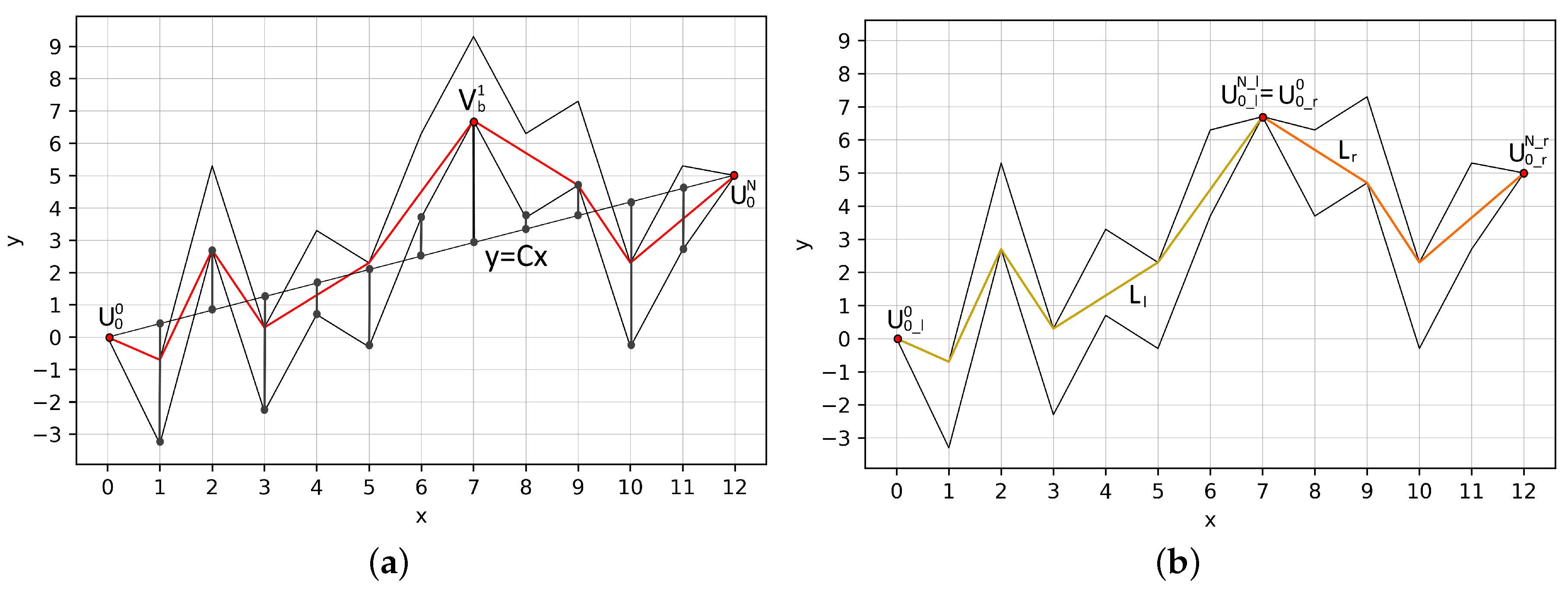
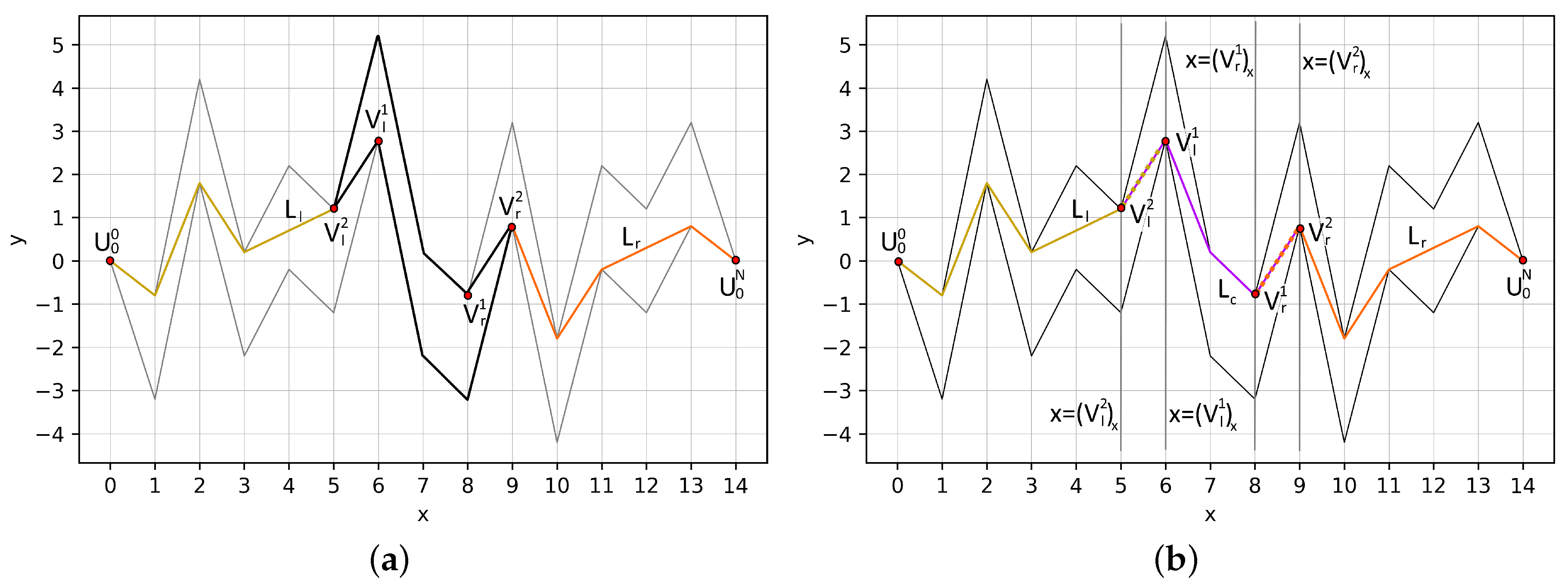
4.1. Exact Dividing of a Tube

Definition 3.

The tube $T_{U_0}(\lambda ,\alpha ,\beta )$ is called balanced if its first and last vertices lie at a zero horizontal level, i.e., $U_0^0=U_0^N=0$.

We call the points $U_0^0$ and $U_0^N$ external vertices of the tube. All other points of the tube are referred to as internal vertices. Consider the highest internal vertices of the tube bottom boundary. Let M be the number of these points, $0\le M\le N-1$. Denote these points by $V_b^i=(x_{V_b}^i,y_{V_b}^i),V_b^i\in B_{bottom},$$i=1,\dots ,M$. In a similar manner we introduce the global minimum points $V_t^j=(x_{V_t}^j,y_{V_t}^j),V_t^j\in B_{top},$$j=1,\dots ,m,0\le m\le N-1$ on the top boundary of the tube, m is number of these points.

Let us consider the bottom boundary of a balanced tube and suppose that the number of global maximum points $M>0$. Figure 9a shows a balanced tube (i.e., $U_0^0$ and $U_0^N$ belong to the same horizontal level $y=0$). The vertices $V_b^1,V_b^2$ of the bottom tube boundary that lie on the horizontal level $y=3.7$, whereas the vertices $V_t^1,V_t^2$ of the top tube boundary lie on the horizontal level $y=-1.7$. The extremal curve L (red) runs through these four vertices.

Proposition 2.

The extremal curve L contains all points $V_b^i,i=1,\dots ,M$.

Proof. 

All points $V_b^i,i=1,\dots ,M$ lie on the same horizontal level $y=y_{V_b}^1=\dots =y_{V_b}^M>0$. Since the tube is balanced, the last tube vertex lies on the zero horizontal level. If L does not pass trough at least one of the points $V_b^i$ then L not be able to reach the zero horizontal level. This follows from the conditions of Remark 3. □

Corollary 1.

The curve L passes through all global minimum points $V_t^j,j=1,\dots ,m$ of the tube top boundary.

Definition 4.

All described global maximum and minimum points are called dividing points.

Note that the initial tube is separated into several parts by dividing points. For each tube part its taut string can be constructed independently.

Remark 6.

If $M=0$ and $m=0$ (i.e., there are no internal global maximum points on the bottom boundary of the tube and there are no internal global minimum points on the top boundary of the tube), then line L runs straight from the first vertex $(x_0,U_0^0)$ to the last vertex $(x_N,U_0^N)$ of the tube, see Figure 9b. If $M+m>0$ then, by Proposition 2 and Corollary 1 there is at least one dividing point.

Let C denote the following constant:

$$C=\frac{{\sum }_{i=1}^N{\alpha }_i{u}_0^i}{{\sum }_{i=1}^N{\alpha }_i}.$$

(40)

Proposition 3.

A tube can be transformed into a balanced tube by linear transformation $F:(x,y)\mapsto (x,y-Cx)$. The taut string of a initial tube is also mapped onto the taut string of a balanced tube by the linear transformation.

Proof. 

Let us consider a modified discrete function ${\tilde{u}}_0^i=u_0^i-C$, $i=1,\dots ,N$. Consider the correspondent function ${\tilde{U}}_0$. It follows from the constructions of tubes $T_{U_0}(\lambda ,\alpha ,\beta )$ and $T_{{\tilde{U}}_0}(\lambda ,\alpha ,\beta )$ that F maps the first tube to the second one. From the Equation (40) it follows that the second tube is balanced.

Subtraction of the constant C does not change the variational problem (3), therefore, the taut string of initial tube is mapped to the taut string of the balanced tube. □

Corollary 2.

Any interior positive maximum point of the bottom tube boundary of a balanced tube is mapped by the inverse linear transformation $F^{-1}$ to a vertex with the maximum vertical distance from the curve connecting the first and last vertices of the initial tube.

Figure 10a shows that the line $y=Cx$ connects first and last vertices of the tube and the distances between the curve and interior vertices of the bottom tube boundary. The extremal curve L (red) contains the vertex $V_b^1$.

Let us choose one vertex $V=(V_x,V_y)$ from the set $\{V_b^1,\dots ,V_b^M,V_t^1,\dots ,V_t^m\}$, and consider the discrete functions $U_{0\_l}=\{U_0^0,\dots ,V\}$, $U_{0\_r}=\{V,\dots ,U_0^N\}$ and the corresponding tubes $T_l$, $T_r$. We construct the extremal curves $L_l$ and $L_r$ for the tubes $T_l$ and $T_r$, respectively.

Figure 10b shows the left extremal curve $L_l$ (yellow) and right extremal curve $L_r$ (orange), the union of these two curves gives the line L of the initial tube (red color in Figure 10a).

Remark 7.

It follows from Propositions 2 and 3 that the union of $L_l$ and $L_r$ is the extremal curve L of the initial tube $T_{U_0}(\lambda ,\alpha ,\beta )$.

The above formulated results can be exploited to design an efficient parallel algorithm for the total variation regularization. The performance of the parallel algorithm in terms of processing speed depends on discrete functions being processed and may be higher than that of the Condat’s algorithm [18] for typical discrete functions with a sufficiently large number of elements. The formulated algorithm has the following drawbacks:

(1)

the dividing vertex can be placed near first or last tube vertices;

(2)

it necessary to pass through all discrete functions $U_0$ to find the dividing vertex.

Remark 8.

Since a tube typically has one vertex on the bottom boundary and one vertex on the top boundary with the maximum vertical distances (up and down, respectively) from the straight line connecting the first and last vertices of the initial tube, then the tube can be easily divided into three (two, if one of these vertices coincides with the first or last vertices of the tube) subtubes. Each subtube can be divided into sub-subtubes and so on.

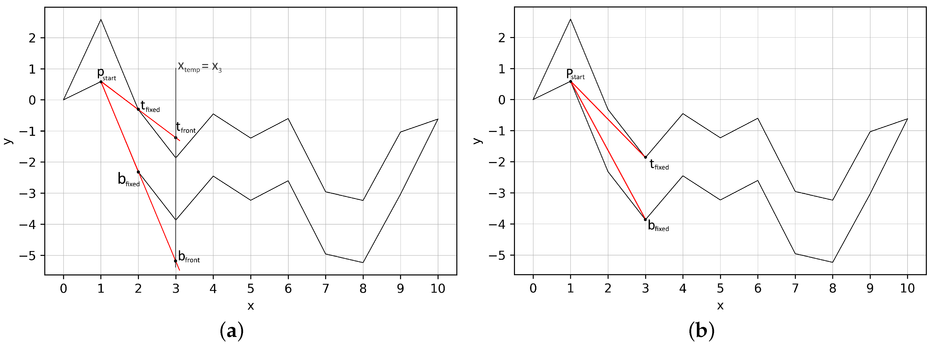
4.2. Fixed Position Dividing a Tube

Let c denote the center point of the tube $T_{U_0}(\lambda ,\alpha ,\beta )$, $c=\left[\frac{N}{2}\right]$. Consider the discrete functions $U_{0\_l}=\{U_0^0,\dots ,U_0^c\}$ and $U_{0\_r}=\{U_0^c,\dots ,U_0^N\}$ and the corresponding tubes $T_l$ and $T_r$. We construct the extremal curves $L_l$ and $L_r$ for tubes $T_l$ and $T_r$, respectively. Let us consider the curve $L_l$. We find a segment of the curve $L_l$ such that the point $U_0^c$ and $V_l^1$ are the last and first vertices of of the segment, respectively. The vertex $V_l^1$ is nearest point to the vertex $U_0^c$ of $L_l$, which belongs to the tube boundary. Let us find also the vertex $V_l^2$, which is the closest point of $L_l$ to the vertex $V_l^1$ (from the left). By the same way we find the vertices $V_r^1$ and $V_r^2$ (to the right from vertex $U_0^c$). Consider the tube $T_c$ with first vertex $V_l^2$ and last vertex $V_r^2$. Let us construct the extremal curve $L_c$ of the tube $T_c$. Consider two pairs of vertical curves $P_l=\{x={\left(V_l^1\right)}_x,x={\left(V_l^2\right)}_x\}$ and $P_r=\{x={\left(V_r^1\right)}_x,x={\left(V_r^2\right)}_x\}$.

Proposition 4.

If a part of $L_c$ coincides with a part of $L_l$ for $x:{\left(V_l^2\right)}_x\le x\le {\left(V_l^1\right)}_x$ and a part of $L_c$ coincides with part of the line $L_r$ for $x:{\left(V_r^1\right)}_x\le x\le {\left(V_r^2\right)}_x$, then the union of the part of $L_l$ (from $U_0^0$ to $V_l^2$) and $L_c$ and the part of $L_r$ (from $V_r^2$ to $U_0^N$) coincides with the true extremal curve L of the initial tube.

Proof. 

If the two nearest vertices of extremal curves lying on the tube boundaries are coincidential, then extremal curves fully coincide. □

Remark 9.

Algorithm for constructing the true extremal curve of the tube $T_c$ uses the extension of the tube $T_c$ to the left and to the right until the condiditions described in the Proposition 4 are met.

Remark 10.

For special types of discrete functions the central tube $T_c$ may coincide with the initial tube T, but for typical discrete functions it is often sufficiently to use the tube $T_c$ in the form described in Proposition 4.

Remark 11.

Dividing a tube into two or more subtubes allows to use parallel computation for solving the variational problem (3). Note that the Condat algorithm [18] can also be parallelized by the proposed method.

Figure 11a shows the initial tube T and its extremal curve L (red). Vertical line $x=c$ passes through the middle of the tube. The point $U_0^c$ is the last vertex of the subtube $T_l$ and the first vertex of the subtube $T_r$. Figure 11b shows the extremal curves $L_l$ (yellow) and $L_l$ (orange).

Figure 12a shows the central subtube $T_c$ (black). Vertices $V_l^q$ and $V_l^2$ determine two straight elements of the left part of the extremal curve $L_c$ (similar to the vertices $V_r^1$ and $V_r^2$). Figure 12b shows that the straight element of the curve $L_c$ lying between the vertices $V_l^1$ and $V_l^2$ coincides with the corresponding part of the curve $L_l$, the straight element of the curve $L_c$ lying between the vertices $V_r^1$ and $V_r^2$ coincides with the corresponding part of the curve $L_r$. This means that the union of $L_l$ (from $U_0^0$ to $V_l^2$), $L_c$ and $L_r$ (from $V_r^2$ to $U_0^N$) coincides with the true extremal curve of the tube.

4.3. Computer Simulation

The objective of computer simulation is to compare with respect to processing time the three proposed algorithms; that is, (1) the linearized taut string algorithm (LTS) described in Section 3, (2) the exact dividing a tube (ExD) and (3) the fixed position dividing a tube (FxD). We compare the processing time of these algorithms. The test discrete functions $u_0$ are generated by the algorithm described in [18]. We consider discrete functions consist of $1\times {10}^5,2\times {10}^5,\dots ,20\times {10}^5$ points. For each function size, we conduct 50 experiments and take the average value of the processing time. The average value is used as an estimate of the processing time for a given size. The obtained results in milliseconds are shown in Figure 13. One can observe that the FxD algorithm is the fastest among all the tested algorithms.

5. Relatively Convex Tubes and Their Properties

In [27,28,29] are described some properties of exact solutions to the standard 1D TV regularization problem (which corresponds to the variational problem (3) with respect to the functional (4) and an algorithm based on these properties. Let us consider the variational problem (3) with the weighted functionals $J_v$ (5) and $J_{vh}$ (6). Note that the properties of exact solutions are true for functional (4), but they may not be true for functionals (5) and (6). Now we state sufficient conditions when these properties are true. These conditions are given in terms of the corresponding tubes.

Definition 5.

A tube $T_{U_0}(\lambda ,\alpha ,\beta )$ is called relatively convex if the corresponding tube $T_0(\lambda ,\alpha ,\beta )$ (with the horizontal central curve $C_0$) bounds a convex domain in ${\mathbf{R}}^2$.

Remark 12.

The condition of relative convexity of the tube $T_{U_0}(\lambda ,\alpha ,\beta )$ means that

$$\frac{\lambda ({\beta }_k-{\beta }_{k-1})}{{\alpha }_k}\ge \frac{\lambda ({\beta }_{k+1}-{\beta }_k)}{{\alpha }_{k+1}},$$

(41)

where $k=1,\dots ,N-1$, and here we suppose that ${\beta }_0={\beta }_N=0$.

Remark 13.

If the central curve $C_0$ of a relatively convex tube has a jump up in the neighborhood of the point $(x_k,U_0^k)$ then the bottom boundary of the tube has also a jump up for the vertical level $x=x_k$ too. If the central curve $C_0$ of a relatively convex tube has also a jump down in the neighborhood of the point $(x_k,U_0^k)$, then the top boundary of the tube has a jump down for the vertical level $x=x_k$ too.

5.1. Intervals of Constancy of the Extremal Function $u_{*}$

Proposition 5.

Let consider a part of the relatively convex tube bounded by the vertical lines $x=x_k$ and $x=x_m$. Suppose that the corresponding part of the central curve $C_0$ is a straight line. Then the corresponding part of the extremal curve L is also a straight line.

Proof. 

The considered part of the top boundary of the tube has jumps down only, thus the corresponding part of the extremal curve cannot jump here according to Remark 3. For the same reason, the extremal curve can not jump down here. Therefore, this part of the extremal curve L is a straight line. □

Corollary 3.

Suppose that the conditions (41) are satisfied. In this case, if the given function $u_0^i$ is constant for $i=k,\dots ,m$, then the extremal function $u_{*}$ is also constant.

Proof. 

The constacy part of the function $u_0$ ($u_{*}$) corresponds to straight part of the piecewise curve $C_0$ $\left(L\right)$. □

5.2. Jumps of the Functions $u_0$ and $u_{*}$

We say that the function $u_0$ has a jump up (jump down) at the point k, if $u_0^k<u_0^{k+1}$ ($u_0^k>u_0^{k+1}$). By the same way we define jumps for the function $u_{*}$.

Proposition 6.

Suppose that the conditions (41) are satisfied. In this case, the types of jumps of the extremal line L cannot be opposite to the types of jumps of the initial function $u_0$.

Proof. 

Suppose for instance, that $u_0$ has jump up at the point k. Then the function $U_0$ has jump up in the neighborhood of the point $(x_k,U_0^k)$. It follows from Remark 13 that the bootom boundary of the tube has a jump up here too. Then it follows from Remark 4 that the extremal curve L cannot have jump down here. Thus $u_{*}$ can not have jump down at the point k. □

Remark 14.

The obtained property reduces the variational problem (3) to a variational problem for a smooth functional (and linear constraints in form of inequalities).

Note that if a tube is not relatively convex, then intervals of constancy of the function $u_0$ can be broken in the function $u_{*}$. In addition, the types of corresponding jumps can be opposite in the functions $u_0$ and $u_{*}$. Figure 14a shows the original discrete function $u_0$ (blue) and its intervals of constancy. The function $u_0$ has three such intervals: $[1;2]$, $[3;4]$ and $[5;6]$. Let consider the variational problem (3) with the functional $J_v$ with the following values of parameters $\beta$: ${\beta }_1=1.0;{\beta }_2=0.3;{\beta }_3=4.0;$${\beta }_4=5.0;{\beta }_5=0.7$. The corresponding vertically nonuniform tube and the extremal curve L (red) are shown in Figure 14b. The extremal function $u_{*}$ is shown in Figure 14a (red). One can observe that, the types of jumps of the intervals of constancy of the functions $u_0$ and $u_{*}$ are opposite for the intervals $[1;2]$ and $[3;4]$. Additionally, the interval of constancy $[5;6]$ of the function $u_0$ is broken in the function $u_{*}$.

5.3. Semigroup Property of Exact Solutions

Denote by $U^{\lambda }\left(U_0\right)$ a solution of the system of Equations (26) with the conditions (28). A semigroup property holds for relatively convex tubes.

Proposition 7.

For relatively convex tubes the following condition holds:

$$U^{t+\tau }\left(U_0\right)=U^t\left(U^{\tau }\left(U_0\right)\right),$$

(42)

where $t\ge 0$ and $\tau \ge 0$.

Proof. 

Consider an extremal curve $U^t\left(U^{\tau }\left(U_0\right)\right)$ of the relatively convex tube $T_{U^{\tau }\left(U_0\right)}(t,\alpha ,\beta )$. Suppose that the extremal curve has a jump down for the vertical level $x=x_k$. Then the extremal curve intersects the bottom boundary here (by Remark 3), and the bottom boundary of the tube has also a jump down here. According to Remark 13 the central curve of the tube has also a jump down here. This central curve is the extremal curve of the tube $T_{U_0}(\tau ,\alpha ,\beta )$. Thus, the considered vertex lies on the bottom boundary of the tube $T_{U_0}(\tau ,\alpha ,\beta )$. Therefore, this vertex belongs to the bottom boundary of the tube $T_{U_0}(t+\tau ,\alpha ,\beta )$. In a similar manner, we can consider of jumps up. Note that the extremal curve $U^t\left(U^{\tau }\left(U_0\right)\right)$ lies inside the tube $T_{U_0}(t+\tau ,\alpha ,\beta )$. Thus, this curve is the extremal curve of the tube in accordance with Remark 3. □

Remark 15.

The semigroup property of exact solutions for 1D discrete TV regularization is nontrivial and takes place for the convex tubes only. In the particular case of variational problem (3) for the functional (6), which corresponds to 2D TV regularization problem for radially symmetric functions (7), this property follows from the paper [30]. The semigroup property helps us to design algorithms for solving the variational problem (3) with the functional $J_{vh}$ [31].

6. Conclusions

In this paper, we proposed three tube-based taut string algorithms for total variation regularization. Various types of tubes were considered: uniform, vertically nonuniform, vertically and horizontally nonuniform. The proposed geometric approach was used to speed-up TV regularization processing by dividing the tubes into subtubes, followed by independent and parallel processing. We introduced the concept of a relatively convex tube and described the relationship between the geometric characteristics of tubes and exact solutions to the TV regularization problem. We have shown that the properties of exact solutions can be used to design efficient algorithms for solving the TV regularization problem. The performance of the proposed algorithms in terms of processing time was discussed and illustrated by computer simulation. The results of this work can be used in various applications. Future work will include an extension of the proposed approach to complex-valued or multi-valued signals and to generalized forms of the TV [32]. The extension to data of higher dimensions, such as 2D images or graphs, also deserves further study [33].

References

1. Rudin, L.; Osher, S.; Fatemi, E. Nonlinear total variation based noise removal algorithms. Physica D 1992, 60, 259–268. [Google Scholar] [CrossRef]
2. Little, M.; Jones, N. Generalized methods and solvers for noise removal from piecewise constant signals. I. Background theory & II. New methods. Proc. R. Soc. A 2011, 467, 3088–3114. [Google Scholar]
3. Acar, R.; Vogel, C. Analysis of bounded variation penalty methods for ill-posed problems. Inverse Probl. 1994, 10, 1217–1229. [Google Scholar] [CrossRef]
4. Allard, W. Total variation regularization for image denoising I. Geometric theory. SIAM J. Math. Anal. 2008, 39, 1150–1190. [Google Scholar] [CrossRef] [Green Version]
5. Allard, W. Total variation regularization for image denoising, II. Examples. SIAM J. Math. Anal. 2008, 1, 400–417. [Google Scholar] [CrossRef] [Green Version]
6. Allard, W. Total variation regularization for image denoising, III. Examples. SIAM J. Imaging Sci. 2009, 2, 532–568. [Google Scholar] [CrossRef]
7. Boyd, S.; Vandenberghe, L. Convex Optimization; Cambridge University Press: New York, NY, USA, 2004. [Google Scholar]
8. Shang, Y.; Ye, Y. Fixed-Time Group Tracking Control With Unknown Inherent Nonlinear Dynamics. IEEE Access 2017, 5, 12833–12842. [Google Scholar] [CrossRef]
9. Shang, Y.; Ye, Y. Leader-Follower Fixed-Time Group Consensus Control of Multiagent Systems under Directed Topology. Complexity 2017, 2017, 3465076:1–3465076:9. [Google Scholar] [CrossRef] [Green Version]
10. Meyer, Y. Oscillating Patterns in Image Processing and Nonlinear Evolution Equations: The Fifteenth Dean Jacqueline B. Lewis Memorial Lectures; American Mathematical Soc.: Providence, RI, USA, 2001; Volume 22. [Google Scholar]
11. Chambolle, A.; Duval, V.; Peyre, G.; Poon, C. Geometric properties of solutions to the total variation denoising problem. arXiv 2016, arXiv:1602.00087. [Google Scholar] [CrossRef] [Green Version]
12. Caselles, V.; Chambolle, A.; Novaga, M. The discontinuity set of solutions of the TV denoising problem and some extensions. Multiscale Model. Simul. 2007, 6, 879–894. [Google Scholar] [CrossRef] [Green Version]
13. Ring, W. Structural properties of solutions to total variation regularization problems. ESAIM Math. Model. Numer. Anal. 2000, 34, 799–810. [Google Scholar] [CrossRef] [Green Version]
14. Chambolle, A.; Pock, T. An introduction to continuous optimization for imaging. Acta Numer. 2016, 25, 161–319. [Google Scholar] [CrossRef]
15. Davies, P.; Kovac, P. Local extremes, runs, strings and multiresolution. Ann. Statist. 2001, 29, 1–65. [Google Scholar] [CrossRef]
16. Johnson, N. A dynamic programming algorithm for the fused Lasso and l0-segmentation. J. Comput. Graph. Stat. 2013, 22, 246–260. [Google Scholar] [CrossRef]
17. Kolmogorov, V.; Pock, T.; Rolinek, M. Total variation on a tree. SIAM J. Imaging Sci. 2016, 9, 605–636. [Google Scholar] [CrossRef]
18. Condat, L. A direct algorithm for 1-D Total Variation Denoising. IEEE Signal Process. Lett. 2013, 20, 1054–1057. [Google Scholar] [CrossRef] [Green Version]
19. Barbero, A.; Sra, S. Modular proximal optimization for multidimensional total-variation regularization. arXiv 2017, arXiv:1411.0589v330. [Google Scholar]
20. Barbero, A.; Sra, S. Proximal Optimization for Multidimensional Total-Variation Regularization. J. Mach. Learn. Res. 2018, 19, 1–82. [Google Scholar]
21. Makovetskii, A.; Voronin, S.; Kober, V. A generalized Condat’s algorithm of 1D total variation regularization. Appl. Digit. Image Process. XL 2017, 10396, 103962K. [Google Scholar]
22. Makovetskii, A.; Voronin, S.; Kober, V. A fast one dimensional total variation regularization algorithm. CEUR Workshop Proc. 2017, 190, 176–179. [Google Scholar]
23. Makovetskii, A.; Voronin, S.; Kober, V. A fast total variation regularization algorithm for 2D piecewise constant radially symmetric functions. J. Phys. Conf. Ser. 2018, 1096, 012041. [Google Scholar] [CrossRef]
24. Kober, V.; Makovetskii, A.; Voronin, S.; Karnaukhov, V. A Fast Algorithm of Regularization of the Total Variation for the Class of Radially Symmetrical Functions. J. Commun. Technol. Electron. 2019, 64, 1500–1507. [Google Scholar] [CrossRef]
25. Strong, D.; Chan, T. Edge-preserving and scale-dependent properties of total variation regularization. Inverse Probl. 2003, 19, 165–187. [Google Scholar] [CrossRef]
26. Bauschke, H.P.; Combettes, L. Convex Analysis and Monotone Operator Theory in Hilbert Spaces; Springer: New York, NY, USA, 2011. [Google Scholar]
27. Makovetskii, A.; Voronin, S.; Kober, V. Explicit solutions of one-dimensional total variation problem. Proc. SPIE 2015, 9599, 959926-1. [Google Scholar]
28. Voronin, S.; Makovetskii, A.; Kober, V.; Karnauhov, V. Properties of exact solutions of the total variation regularization functions of one variable. J. Commun. Technol. Electron. 2015, 60, 1356–1359. [Google Scholar] [CrossRef]
29. Makovetskii, A.; Voronin, S.; Kober, V. An efficient algorithm for total variation denoising. Proc. Int. Conf. Anal. Images Soc. Netw. Texts CCIS 2017, 661, 326–337. [Google Scholar]
30. Jalalzai, K. Some remarks on the staircasing phenomenon in total variation-based image denoising. J. Math. Imaging Vis. 2015, 54, 256–268. [Google Scholar] [CrossRef] [Green Version]
31. Makovetskii, A.; Voronin, S.; Kober, V. Total variation regularization with bounded linear variations. In Proceedings SPIE’s 61 Annual Meeting: Applications of Digital Image Processing XXXIX; International Society for Optics and Photonics: Bellingham, WA, USA, 2016; Volume 9971, p. 99712T-9. [Google Scholar]
32. Dumbgen, L.; Kovac, A. Extensions of smoothing via taut strings. Electron. J. Statist. 2009, 3, 41–75. [Google Scholar] [CrossRef]
33. Hinterberger, W.; Hintermüller, M.; Kunisch, K.; Von Oehsen, M.; Scherzer, O. Tube methods for BV regularization. J. Math. Imaging Vis. 2003, 19, 219–235. [Google Scholar] [CrossRef]
Figure 1. Coordinate planes (gray color), graph of the functional J 3 ( u ) (green color), planes corresponding to elements of subdifferential of the functional J 3 ( u ) when u 2 = u 1 (yellow color).
Mathematics 08 01141 g001
Figure 2. Points ( x i , U 0 i ) , i = 1 , , N are defined by the discrete function U 0 ; piecewise linear curve C 0 is shown by the blue dashed line.
Mathematics 08 01141 g002
Figure 3. Curve C 0 (blue dashed line) and vertical λ β i neighborhoods of the vertices ( x i , U 0 i ) .
Mathematics 08 01141 g003
Figure 4. The tube T U 0 ( λ , α , β ) of the function U 0 and corresponding curve C 0 (blue dashed line).
Mathematics 08 01141 g004
Figure 5. (a) The neighborhood of the vertex where L runs straight; (b) the neighborhood of the vertex where L has a jump up; (c) the neighborhood of the vertex where L has a jump down.
Mathematics 08 01141 g005
Figure 6. Taut string (red) in the tube.
Mathematics 08 01141 g006
Figure 7. (a) Scanning cone with t e m p = 3 ; (b) correction of the cone.
Mathematics 08 01141 g007
Figure 8. (a) Scanning cone with t e m p = 4 ; (b) fixed part of the taut string.
Mathematics 08 01141 g008
Figure 9. (a) Internal vertices of a balanced tube, which are global maxima and minima, curve L (red); (b) balanced tube with curve L without jumps.
Mathematics 08 01141 g009
Figure 10. (a) Distances between the line y = C x and interior vertices of the bottom tube boundary, extremal curve L (red); (b) extremal curves L l (yellow) of the left subtube and L r (orange) of the right subtube.
Mathematics 08 01141 g010
Figure 11. (a) The initial tube and its extremal curve L (red); (b) extremal curves L l (yellow) of the left subtube and L r (orange) of the right subtube.
Mathematics 08 01141 g011
Figure 12. (a) Central subtube T c (black); (b) part of the extremal curve L c (purple) between vertices V l 2 and V l 1 coincides with corresponding part of the curve L l , part of the extremal curve L c (purple) between vertices V r 1 and V r 2 coincides with correspondent part of the curve L l .
Mathematics 08 01141 g012
Figure 13. Average processing times for linearized taut string (LTS) (red), exact dividing a tube (ExD) (green) and fixed position dividing a tube (FxD) (blue) algorithms in milliseconds. On the horizontal axis, the corresponding sizes of discrete functions are marked.
Mathematics 08 01141 g013
Figure 14. (a) Original discrete function u 0 (blue) and its intervals of constancy, extremal function u * (red) and its intervals of constancy; (b) the corresponding vertically nonuniform tube (black) and extremal curve L (red).
Mathematics 08 01141 g014