Abstract
This study explains about a serial smart production system where a single-type of product is produced. This system uses an unequally sized batch policy in subsequent stages. The setup cost is not always deterministic, it can be controllable and reduced by increasing the capital investment cost, and that the production rates in the system may vary within given limits across batches of shipments. Furthermore, as imperfect items are produced in long-run system, to clean the imperfectness autonomation policy is adopted for inspection, which make the process smarter. The shipment lot sizes of the deliveries are unequal and variable. In long-run production system, defective items are produced in “out-of-control” state. In this model, the defect rate is random with a uniform distribution which is clean from the system by autonomation. In addition, in the remanufacturing process, it is assuming that all defective products are repaired, and no defective products are scrapped. The main theme of developing this model is to determine the number of shipments and the optimal production lot size to adjust the production rates and decrease the total system cost under a reduced setup cost by considering the discrete investment and make a serial smart production system. A solution procedure along with an advanced algorithm was proposed for solving the model. Numerical examples with some graphical representations are provided to validate the model.
1. Introduction
The managements of a serial or multi-stage production process (MSPP) have fetched an enormous contract of consideration in recent decades. The three main management strategies investigated in pursuit of company goals are strategic, tactical, and operational.
- On a strategic level, the main target of any researcher is how the production process should be devised to optimize the everlasting acquisition of the industry along with a smart production system.
- On a tactical level, researchers have investigated investment opportunities for modernizing and extending production equipment, such as to lower setup costs (SC), to reduce lead times, or to expand available production capacities.
- On an operational level, some methods are developed by researcher to support companies in using specific production machinery as strongly as required. Decisions, that must be made at the viable stage, include determining order and production lot sizes, production sequences, and delivery schedules.
Controlling the production rate is an effective method at the operational level. Basically, the production rate is assumed as constant in any production process. Inventory level may be increased along with high unit production cost (UPC) due to a fixed production rate, which may have a negative impact on the production system. A variable production rate (VPR) can adjust inventory levels to achieve lower production system costs. Managers are increasingly concerned about the control of productivity. Productivity is a crucial indicator of a production line and the performance of the production line is a crucial indicator of the production process. Recently, the evaluation of production line performance has attracted a huge contract of consideration. The production line framework is classified into “serial production lines (SPL)”, “assembly/disassembly lines”, “loop lines”, and “re-entrant lines”. Among these, an SPL is used most widely, such as in the automobile industry and the electronics industry. In the production process, reducing excessive inventory can decrease the costs associated with production, hoarding, and transporting products. With this in mind, the manager must choose the economic lot size.
An imperfect production process (IPP) with buffer inventory and warranty policy was developed by Sana [1]. In recent days, a supply chain model for work-in-process system was presented by Sarkar and Chung [2]. To control work-in-process system, autonomation policy had a great impact proved by Dey et al. [3]. An imperfect production model was developed by Cárdenas-Barrón [4], where single-stage production took places, in the same direction Cárdenas-Barrón [5] developed several models like as Cárdenas-Barrón [6]. The objective of many models is to optimize the total system cost including holding cost (HC), ordering cost (OC), and transportation cost. Many researchers have studied and extended these two inventory models. For example, performance with a random defective rate and imperfect remanufacturing process in a production model (PM) was explained by Chiu et al. [7]. A PM was presented by Jamal et al. [8] in which a single-production system was discussed and regulated the optimal lot size that performed remanufacturing through two methods (online and offline). Maddah and Jaber [9] developed an inventory model with unreliable supply, imperfect quality (IQ), and a screening process and they evaluated the effects of screening facilities and fluctuation of the supply system on the ordered products. An improved solution for manufacturing model along with remanufacturing was introduced by Cárdenas-Barrón et al. [10]. Recently, a two-period supply chain for green product was designed by Dey et al. [11]. Nobil et al. [12] investigated an economic production model (EPM) where the effect of warm-up period on defective products are described in a cleaner production system.
1.1. Research Motivation
The focus of the current work is an important direction in the production system that presented at the basic decision level: to set the rates of production in each stage in accordance with customer demands, to determine the lot sizes of production, the number of shipments to minimize total cost in an imperfect serial-production system. The main aim of any industry is to reduce the total system cost by using different policies. For any production system, setup is one of the most important necessity. Thus, for any production process, setup and cost related to setup play a major role and this is the reason that several researchers try to develop different models with different polices to reduce setup cost. Sometime investments can reduce different basic costs related to any perfect/imperfect production system. Several researchers proved that an investment can reduce setup cost as well as total system cost (Dey et al. [13], Huang et al. [14], Ouyang et al. [15], Sarkar and Chung [2]). In this current study, a target is taken to reduce setup cost along with total system cost for an imperfect serial production system by some investment.
On an operational level, the reduction of surplus inventory can lead to many prosperities. Reducing inventory can reduce the total cost in a production system. In an actual production process, the production rate varies within a certain limit, which in turn changes the unit production cost (UPC). The managers of production can precisely accustom the speed of processing of the production line to meet customer demands. At the same time, inventory build-up as well as the total system costs of a production system influenced by production rate. The variability of the production rate is a real factor for production system in general, but most previous works have considered production rate to be constant. This is a major drawback to previous studies. Additionally, in production system, SC is an important part of the whole cost. The setup configures all production batch-related work. Most studies have considered SC as fixed. In fact, SC can be reduced by increasing investment, and reducing SC has become an increasingly attractive approach. For example, a pizza making shop (7-th Street Pizza) offers of giving pizza to each customers within 30 min. If there are several customers and all orders come together, then managing all orders within 30 min are really difficult for them. As a result, the pizza can be delivered to them without any money as per the policy of the company. Thus, they use a controllable production rate within their production setup such that the production rate can be controllable within some certain limit. It will remove the shortages from the systems. For making the controllable production process, they have to invest some fixed costs to make the perfect setup for it. This is known as discrete SC investment. This fund will help to make the production system smarter such that there will not be any free pizza from 7-th Street Pizza shop. This study considers similar like serial production system to reduce the system cost.
1.2. Research Objectives
This is an extended work of Glock [16] to an imperfect serial production system (ISPS) with a random, uniform distributed defective rate, in which all scrap items are repaired in the same cycle. It is assumed that the SCs can be reduced by introducing the investment. The production rates are adjusted during the production process. The backordering consideration is relaxed in this work. The aim of this model is to develop a decision support model for determining the production rates in an ISPS. The proposed model deals with the following decision problems:
- (1)
- Determine the optimal production lot size (OPLS), Q, which can be produced in a single production cycle. In the manufacturing sector, to achieve more profit, companies have to determine the optimal production lot size that minimizes the total system costs such that the resources can be used effectively.
- (2)
- Determine the number of shipments. Unnecessary transport equipment increases the total cost in a production system, whereas setting the appropriate number of shipments reduces the cost.
- (3)
- Clarify the rate of production for each production stage. Managers can control the speed of processing for the production process to reduce the excessive inventory.
- (4)
- Determine the SC at each stage as related to the investment cost (IC). When manufacturing industries reduce the SC, it directly affects the total system cost up to a certain limit, but huge investments again increase the total system cost.
Most commonly, any production process produced the perfect quality item at starting, but in a long run system, imperfect items maybe produced by machine. To keep the brand image of company, most of the production process has gone through an inspection policy and remanufacturing are done to make the imperfect product as perfect. Most of the researcher considered a human inspection to detect the imperfect product, where different types of error may occur (See Sarkar and Saren [17]). The inspection error may occur due to new inspector or unskilled inspector, that is learning error can effect in the cost of the system proved by Khan et al. [18]. To make an inspection error-free serial smart production system (SSPS), an autonomation policy is utilized for inspection. Uses of autonomation policy make the production process smarter.
2. Literature Review
Three streams of research frame the current study.
- One stream is the study of an imperfect multi-stage production system (IMSPS). In an actual production process, defective products are inevitable, and managers must control the cost of a business operation in their presence.
- Another area of inquiry seeks to reduce SC through an added investment cost. Although many studies have considered the fixed SC, it may be diminished through an extra investment and thus it is controllable.
- Researchers have also investigated the situation of VPR on performance in multi-stage inventory models and examined how varying the production rates leads to different types of costs in the system. As a result that the UPC changes as production rates are varied, managers must select the appropriate production rate for a given customer demand. This area of research also investigates the effect of changing production rate on different types of costs in the system, such as holding, inventory cost, etc.
The three streams of research are summarized in Table 1, showing the major research gaps addressed by the present study as IMSP, SC reduction, and production rate.

Table 1.
Contribution of previous author(s).
The multi-stage production is used have to achieve a large amount of products in the supply chain management.
2.1. Imperfect Production Process
Most of the researchers investigate some single-stage production system instated of imperfect multi-stage production system along with reduced SC. For reduction of SC, a discrete investment is implied. To study a single-stage production system, researchers usually develop inventory models, most of which incorporate a constant defective rate. Some studies have included remanufacturing of defective products. To achieve the highest profit by determining the rate of production and optimal reliability of the product, Sarkar et al. [25] formed the defective rate by using control theory. A random defective rate (RDR) in a single-stage production process was considered by Chiu et al. [7] and Sarkar et al. [26] with a remanufacturing opportunity. A production model with shortage and screening constraint was investigated by Wee et al. [27], in which they considered that the production process may produce imperfect quality items. Recently, Tayyab et al. [28], Tayyab et al. [29] developed two multi-stage models where they discussed about a lean manufacturing system. Tayyab et al. [28] discussed about imperfect production with fuzzy demand pattern and in the next model Tayyab et al. [29] considered uncertainty only. An improved way was proposed by Kim et al. [30] for calculating the imperfect product during long run system. Similarly, a mixed model for single-vendor, along with a single-buyer for defective production process was reformulated by Dey and Giri [31], the effect of learning has a great impact in inspection and was also discussed in this model. Following the same way, Tiwari et al. [32] developed a sustainable inventory model with the consideration of carbon emission. Tiwari et al. [33] again extended this model by considering a multi-item sustainable green production system. They also considered the concept of trade-credit and partial backlogging. A few works have considered imperfect multi-stage production system. Sarker et al. [23] studied two remanufacturing strategies for a IMSPS: one strategy was to perform the remanufacturing within the same cycle in which the defect is discovered, and the other was to do the remanufacturing after n-cycles. Kim and Sarkar [34] introduced a method to reduce the defective items to an almost zero level within the production framework for a complex MSPS with improved quality. A multi-level consignment stock scheme (MLCSS) for CLSC was developed by Taleizadeh and Moshtagh [35], where production process produced imperfect quality items with lost sales. Sarkar [36] introduced the optimum way to remanufacturing for defective products in a multi-stage multi-cycle production system (MSMCPS) with a discrete investment for SC reduction under random defective production rate. Most of the researchers considered imperfect production process or multi-stage production process for imperfect manufacturing system along with manual inspection to detect defective product. Some researchers considered different type of error in inspection or learning effect in inspection [17,18,31] but no one cared about how this inspection error can be removed. In this model, the whole inspection is done automatically by a machine, that is the concept of autonomation policy is utilized to identify the defective items which make an error-free inspection system. Thus, this is a pioneer attempt to make an error-free inspection for the imperfect multi-stage production model. Thus adaptation of autonomation policy is making the system smarter which is always profitable for any production industry.
2.2. Setup Cost Reduction
The cost to establish a production system along with the configuration of all production with batches related works is called SC. As SC is directly linked to the total system cost of production, it must be reduced anyhow to optimize the total system cost. Many studies considered SC as fixed. In reality, SC can be controlled and it can be diminished through an extra capital investment. The investment cost is the capital cost of the firm’s investment in the production. Setup cost reduction can improve the competitiveness of enterprises, improve customer service, reduce waiting time, and improve production efficiency. To reluctant the total system SC for a basic inventory model (BIM), capital investment plays a major role, first discussed by Porteus [37]. Nori et al. [38] studied the relationship between the SC and the amount of capital investment. In uncertain demand environment, Hong et al. [39] discussed three production policies for dynamic SC reduction with an investment. Ouyang et al. [15] utilized a “min-max distribution-free” technique to find optimum result, where thelead time demand (LTD) follows a normal distribution (ND) with optimized reorder point, SC, lot size, and process quality. They discussed about a method to reduce SC by investing some initial capital. Dey et al. [13] described a production model with an IMP and diminished SC. They discussed several cases of product-specific quality improvements and joint-product quality improvement. Sarkar et al. [22] developed a continuous-reviewed model where the process quality was improved and to make the model more realistic service level was considered as constraint, and SC was also reduced. The relationship between investment cost in SC reduction and SC level was initially considered to be continuous. A method was introduced by Sarker and Coates [40] to determine the optimal amount of capital investment to reduce SCs when there is a discrete investments–SC relationship. Recently, Guchhait et al. [41] discussed the impact of investment on SC for an imperfect production process, where warranty policy and shortages takes place.
A controllable production rate improves an inventory build-up and reduces excessive inventory. It increases the flexibility of the supply chain and reduces production inventory and transportation costs. Varying the production rate in a production system affects the inventory in relation to waiting time, and it can control the inventory level in the production stage.
For example, in the food industry, managers should adjust the production rate in the manufacturing process to meet the needs of customers. Managers can ensure that the product is available and not wasted due to overproduction; they can benefit the business by controlling the productivity.
Many authors have considered the production rate as constant, and only a few have considered a VPR. The rigid case model was first introduced by Buzacott and Ozkarahan [42], they considered the problem of assigning two different products to a single machine or two different machines. They assumed that the production rate could be changed and investigated how to determine the optimal production rate. Larsen [43] and Sharma [44] both developed variable demands and production rates in two economic production quantity models. They assumed that demand was dynamic and analyzed how to adjust the production rate in the model. They proved that a reduction in production rate led to reduced inventory build-up and lower inventory holding cost (IHC).
Moon et al. [45] analyzed the flexible case and proposed a model that allowed production rates to be varied. They reduced the production rate to meet the demand while avoiding inventory build-up. Elhafsi and Bai [46] included backorder rate in their model and proved that VPR could reduce the average system cost. A production model of the flexible case was provided by Majumder et al. [21], who considered the production rates and production cost as decision variables for a multi-retailer integrated inventory model. Their research showed that the production rate should be between the demand rate and the ordering quantity to minimize unit production costs. In the same direction Sarkar et al. [47] explained the impact of variable production rate (VPR) for the quality of the product.
A two-stage production system was considered by Glock [48], where he assumed that the products producing in the first stage are used in the second stage. He considered a VPR in the first stage and investigated how VPR influenced the total system cost for both the flexible cases and the rigid cases. Glock [16] extended his own model to a multi-stage from two stage production period line, and he developed a generalized model for equal-sized and unequal-sized batch shipment policy (USBSP) but he ignored about the setup reduction by an investment as controllable production setup is costly and a huge investment is needed there and without initial investment, it is almost impossible.
2.3. Gap in Literature
Most of the existing literature considered imperfect production system with fixed setup cost and manual inspections for identify the imperfectness of the products, which leads to a larger amount of total system cost and may delivered imperfect items to the market due to error in inspection. There are few such imperfect serial models till now considered with a random defective rate, variable setup, and production cost, which can have reduced total system cost and there are no such imperfect serial production models till now considered where machine based autonomation inspection is considered for an error free inspection process. This is a big research gap in this direction. Thus, this proposed research focused on an investment which is used to change the production setup from traditional to flexible production system along with adaptation of autonomation policy for detect the imperfect items, which make an SSPS. The concept of this model is almost the same as Glock [16]. The major differences are that the present work considers an s-stage production system, and a SC reduction is achieved through an added investment along with the adaptation of autonomation policy for inspection, which make the process more smart. Defective items are produced along with the good quality items in this study, whereas Glock [16] investigated the case of multiple stages.
3. Problem Definition, Assumptions, and Notation
3.1. Problem Description
The current study investigates the production process in which a single-type of product is produced in an imperfect s-stage serial production system (ISSPS) with an unequally sized batch shipment policy between subsequent stages. Some PI along with a random percentage of imperfect items will produced. All items are inspected through autonomation policy, and all defective items, which are produced, remanufactured within the cycle (Sarkar et al. [26]). These remanufactured items are transferred to the next stages as perfect quality items. The main problem associated with VPR for an SSPS is described graphically in Figure 1. For example, bicycle parts pass through the production, transportation, assembly, and packaging steps and then from supplier to retailers. Defective items are produced randomly in a uniform distribution. These defective items are remanufactured.
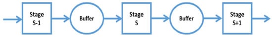
Figure 1.
A three-stage production system with two buffer stocks.
The intention of the managers is to cut down inventory levels at each production stage, decrease the IHC, and overcome unnecessary costs, including those due to defective products, excessive transportation, remanufacturing, and over-production. Sometimes an investment can reduce the total system cost. There are two types of investment that can be performing; one is continuous and another is discrete. In this model, one can easily find that discrete investment for reducing SC is more profitable. Thus, a discrete investment is introduced to reduced production SC along with minimized total system cost. The novelty of the model is that an investment is discretely used to reduce the production SC or finally the total system’s cost and autonomation policy is utilized to detect the imperfect items which make the process more smart with error-free inspection. To change the fixed production rate to controllable production rate, a huge investment is needed to change the whole production setup. Thus, using an investment to change the production setup and finally, reduce the shortages to more profit with the reduced SC each stage, this policy is nowadays taken by several industries. This model solves this problem to show the cost is purely reduced from the traditional production system with constant production rate. The imperfect items are completely inspected through the machine such that an error-free inspection is done that is the concept of autonomation policy is utilized for a serial production process, which is the pioneer attempt to make a SSPS model.
3.2. Basic Assumptions and Notation
To demonstrate the model, the following assumptions are made:
Assumptions
- (1)
- A multi-stage production system for a single-type of items (see Tayyab and Sarkar [24]) is considered with demand rate d and VPR , where . For the VPR, UPC is a function of the production rate (see Sarkar and Chung [2]).
- (2)
- SC at each stage is considered a variable and can be reduced through additional investment (see Dey et al. [13]). Production and remanufacturing are performed at the same production rate (see Sarkar et al. [26]).
- (3)
- The defective rate at all stages is a random variable and defective products are remanufactured (see Sarkar et al. [26]) to make as perfect as well as shortages are not allowed.
- (4)
- All defective products are inspected through a machine instead of human begins that is autonomation policy is adopted for inspection, which make the production process smarter (see Dey et al. [3]).
In addition, the following notation is used to formulate the problem.
3.3. Notation
| Index | |
| i | number of production batch |
| j | batch size |
| Decision variables | |
| Q | production lot size per production cycle (items) |
| n | number of shipments in a production cycle (integer) |
| production rate of stage-s per production cycle, where (items per unit time, where ) | |
| investment per production run required to achieve setup cost of stage S ($/stage/setup) | |
| Parameters | |
| unit production cost of stage-s ($/item) | |
| inventory holding cost per unit per unit time in the buffer stock ($/item/unit time) | |
| S | number of production stages (integer) |
| D | total demand in the planning period (units) |
| inspection cost of the production stage-s ($/item/stage) | |
| transportation costs per shipment at stage-s ($/shipment/stage) | |
| original setup cost before any investment is made at each stage ($/stage/setup) | |
| setup cost per production run, which is a strictly decreasing function of , with = , where is a known parameter ($/stage/setup) | |
| time component related to the inventory at stage s for i th production batch(time unit) | |
| production rate at stage s (unit/stage) | |
| shipment batch size at stage s (unit/batch) | |
| expected value for the random defectiveness, which follows a uniform distribution and , where, R is random defectiveness, , and are scaling parameters | |
| scaling parameters i.e., , , and are scaling parameters | |
3.4. Mathematical Model
This model represents an MSPS. A single-type of products is produced in this SPS. During the production process, defective products are produced at a random rate and are remanufactured to regenerated them as some good quality products. In this model, a discrete investment is utilized to diminished the SC for the MSPS and the production rate is assumed as controllable.
The target of the supplier is to minimize the total system costs, which consist of the following costs.
(1) Inventory holding cost (IHC)
Unequally gauged bundles are shifted to subsequent stages and the gauge of the j-th bundle bank on the gauge of the first parcel and production rate of batches 2 to n.
The size of each batch shipment is
The total quality of shipment lots per cycle is calculated as follows:
At stage s, time-weighted inventory can be expressed as [see for instance [16]
If , then the related inventory time design are shown in Figure 2, where the bold line indicates the original production rate and the dashed line indicates a reduced production rate.
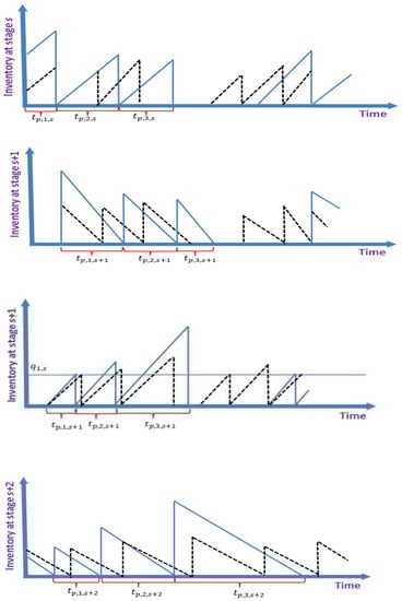
Figure 2.
Inventory versus time plots for unequally sized batch shipments.
Thus, the total inventory carrying cost can be calculated as
(2) Total production cost (TPC)
To produce an item some production related costs are involved. Thus, the UPC of the product is assumed to be convex in its production rate, which is treated as a decision variable. Thus, one can assume that the UPC is the function of production rate, specified by Eiamkanchanalai and Banerjee [49]; that is,
Therefore, in this model, the total production size Q multiplied by the UPC over all S stages in the planning period provides the total production cost as
(3) Online autonomated inspection cost per cycle (OAICPC)
Inspection cost is incurred through the inspection process. Each stage has the same inspection cost. is the unit inspection cost per item, the TIC for the stage-s is the summation of the IC of a batch with quantity Q and remanufactured products. It is assumed that, in each batch shipment, the defective rate is random and follows a uniform distribution (see Sarkar et al. [26]). Thus, one can conclude that the total inspection cost is as follows:
where, , and are the scaling parameters when defective rate follows a uniform distribution.
(4) Remanufacturing cost per cycle (RCPC)
It is assumed that, in each batch shipment, the defective rate is random and follows a uniform distribution (see Sarkar et al. [26]). The total remanufacturing cost is calculated as
(5) Transportation cost per cycle (TCPC)
In this model, an unequally sized batch policy is used to ship the products between subsequent stages. At each stage, the transportation cost is , and the total number of shipments is n. Thus, we calculate the total transportation cost as follows:
(6) Setup cost per cycle (SCPC)
Build-up is a basic concern for whole production process to produced raw materials for manufacture a perfect products. The reduction in SC for a production stage is . In this model, an added investment cost is considered to reduce the SC. Hence, , where is the investment cost at each stage. The total SC for an S-SPS can be obtained as
(7) Investment for setup cost reduction per cycle (ISCRPC)
By summing the investment cost over all S stages and multiplying by the planning period , one can obtain
The total system cost is given by
Substituting the values of these costs, one can have
4. Solution Methodology and Solution Algorithm
This section contained the solution procedure of this model. A brief description of solution methodology is discussed in this section. The combination of algebraic optimization technique and line search algorithm technique are used to solve this model. Some numerical examples also given in this section to test the global optimality of the solution. This section is subdivided as follows:
4.1. Solution Methodology
In this section the algebraic optimization technique describe briefly as follows:
Algebraic Optimization Technique
One can consider a quadratic equation as
where, A, and B are positive constant.
The Equation (13) can be rewritten as
Since, A is the positive constant and is always positive due to the square, thus, first term of the Expression (14) is positive and the Expression (14) is positive.
Now the Expression (14) provided the minimum value only when
Thus, the minimum value at is .
This process is known as the algebraic optimization technique.
Now, in this model, for given values of n, , and , Equation (12) can be written in the form
See Appendix A for the value of .
Now the expression
will be minimum when , and minimum cost is .
Therefore, is minimum when
The minimum cost is
For the value of , one can cover a line search algorithm within the intervals . Further, one can calculate a solution for n using the following condition:
4.2. Solution Algorithm
An algorithm SPDS is developed to find the optimum value of the decision values as follows:
SPDS Algorithm
| Step 1 | Input all parametric values. |
| Step 2 | For each . Set and search that minimizes . Set , , and . Set . |
| Step 3 | Search and that minimize . If , go to Step 4. |
| Step 4 | Set , , and , and . Go to Step 2. |
| Step 5 | Find from Equation (12) and finally obtain . |
5. Numerical Experiments
To demonstrate the effect of VPR on an ISPS with bundle parcels and investment cost, one can perform a numerical experiment. The following data are obtained from Glock [16] and Sarkar et al. [26], and the values are units/year, , , /unit. A set of solved test problems is provided in Table 2.
Table 2.
Test problems used for computational experiments.
From Table 2, for the original SC at each stage, one can have two cases: Case 1 and Case 2 . In addition, the parametric value of the maximum, and minimum production rate is provided in Table 2. Then, using optimization tools, one can find that original setup cost is reduced under the investment, which was provided in Table 3. Table 3 shows that the original SC can be reduced through added investment cost, and the SC reduction versus investment has three situations. From Table 3, initial setup cost, i.e., when there was no investment are , , , and , , , those initial setup costs are obtain from Table 2. When the investment is , then the cost reduced and the reduced costs are , , , , , and . That is setup cost reduced by , , , , , and when investment is .
Table 3.
Setup cost versus investment data.
Similarly, when the investment is , then the cost reduced and the reduced costs are , , , , , and . That is setup cost reduced by , , , , , and when investment is .
Again, when the investment is , then the cost reduced and the reduced costs are , , , , , and . That is setup cost reduced by , , , , , and when investment is . It is clear that 1st set of initial setup cost can be reduced by , , when investment is , and setup cost can be reduce by , , and when the added investment is and setup cost is reduce by , , for the added investment . Similarly, the second set of initial setup cost can be reduced by , , when investment is , can be reduced by , , and when the added investment is , and setup cost is reduced by , , for the added investment . The reduction in setup cost for two different sets of data are graphically presented in Figure 3.Thus, an added investment can reduce the total system setup cost, which is graphically shown in Figure 3. How investment of , , reduced total system setup cost for six different data sets are graphically presented in Figure 3.
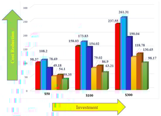
Figure 3.
Graphical representation of investment versus setup cost reduction.
Analysis of the Mathematical Model
Table 4 provides the optimum results of the model. From Table 4, one can obtain optimal production lot size, optimum shipment numbers, and optimum production rate for stage s. Table 4 shows 6 cases for optimal values. Case 1 is for real data, and Case 2 shows the effect of the IHC for VPR. Increasing the HC leads to higher IHC, which increases the convenience that reaction from the VPR.
Table 4.
Optimum result table.
In Case 3, if the transportation cost increases, the number of parcels n is reduced. Case 4 shows the effect of varying the SC, that also affects the number of parcels in the outlining cycle and the production rate. Cases 5 and 6 show the relationship between the UPC function and the production rate; expanding or depreciating the production rate tends to a stinging expand in production cost.
The optimum result along with optimum decision variable for different investments are provided in Table 5. How different investment can effect in total cost is graphically presented in Figure 4. Table 5 shows the reduction of SC through added investment, where leads to the lowest total system cost except for Case 4. The bold value of Table 5 proves that the total cost was minimum for Case 1, Case 2, Case 3, Case 5, Case 6, when investment is $100, and the costs are $10,449.3, $15,806.9, $11,645.9, $11,291.9, and $11,324.1.
Table 5.
The reduction of setup cost through added investment.
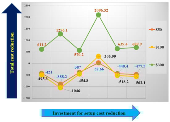
Figure 4.
Effect of investment on total cost.
An investment can reduce setup cost as well as total system cost to a certain limit, and a higher investment can also reduce setup cost (data are given in Table 3), but total system cost can be reduced for investment to a certain limit of investment. From Table 3 it is clear that total setup cost can be reduced by an investment. From Table 5, it is proved that investment can reduce total system cost to a certain limit. After that, total system cost is increased due to high investment. In our model, it is proved that when investment is or , the setup cost is reduced as well as system cost is reduced. When there is no investment, the total system costs for six different situations are , $16,852.9, $12,100.70, , $11,810.10, and 11,886.20 and in this case the setup costs are , , , and , , .
When the investment is , total system cost reduced along with setup cost. In this case the system costs are $10,523.6, $15,964.7, $11,713.70, , $11,369.70, and 11,408.70 and setup cost reduces to , , , and , , .
Again, when investment is , setup costs are reduced along with reduced system cost due to investment. The total system costs due to investment of are $ 10,449.3, $15,806.9, $11,645.9, , $11,291.90, and 11,324.10 and setup costs reduce to , , , and , , .
When investment is , setup costs are reduced but system cost is increased due to high investment. The total system cost due to investment of are $ 11,555.80, $18,129.00, $12,670.90, $11,769.60, $12,449.50, and 12,576.10 but reduced setup costs are , , , and , , .
Thus investment can reduced total system cost up to a certain limit, then again system cost is increased though setup cost is reduced due to high investment, which was proved by the result of Table 5. That mean how much to invest that also very crucial decision for any industry. Thats why, in this model, when the investment is or the setup cost is reduced as well as total system cost also reduced but when the investment is the setup cost is reduced but system cost is increased.
The total system cost is minimum for case 4 without investment. Thus, one can conclude that, in many cases, one can reduce the SC through an added investment. Thus, an investment is really helpful for a serial production system to reduced setup cost as well as reduced total system cost.
The managers of any multi-stage manufacturing industry can benefit from these findings based on random defective rates. Managers can use these findings to determine the optimal production lot size and number of shipments between subsequent stages. They can adjust the production rate in system to meet specific customer demands. It is also notable that adding capital investment cost for the setup decreases the total production system cost. Graphically, it is provided in Figure 4. From Figure 4, it is clear that added investment in setup cost reduced total system cost.
6. Managerial Insights
In this study, it is treated the case where a single-type of product is manufactured in an IMSSPS, with unequally sized bundle parcels. In this system, faulty items are prepared at an arbitrary rate. The production rate can be controlled by a flexible method, which means that the production rate can be motleys during production. In addition, SC is controllable through an added investment cost. The major insights of this study are as follows:
- A controlled production rate can reduce inventory and total system cost. A VPR can help to transfer inventory between stages, which permit the managers to utilize different inventory holding charges in the production system. It reduces the excess inventory for long-time holding.
- Managers can adjust the production rate, which depends on (1) the number of batch shipments, (2) the IHC applicable to the buffer stock, and (3) the transportation cost between stages. Managers can decide easily what should be the production rate during production to meet the customer’s demand on time.
- Setup cost can be controlled and reduced through added investment cost, which reduces the total system cost up to a certain limit. High investment can lead to a high system cost, though setup cost is reduced.
7. Conclusions
The multi-stage imperfect serial production was considered to make complex products with a controllable production rate. The controllable production rate was used to maintain the production in such a way that the shortages did not appear. The result proved that this idea could be easily admissible by any multi-stage production industry to obtain the minimum cost with no shortages. To make the controllable production rate from the traditional production rate, a huge amount of fund were needed to reducing the whole production system. Some discrete investment was used to reduce SC of the system. Results found that the discrete investment really reduced the initial SC and finally the total cost of the system up to a certain limit, but a huge investment again increases total system cost. Due to the combination of controllable production rate and reduced SC, the total cost of the model was minimized with respect to the decision variable at the optimum values.
The major contribution of this work is to inform managers that they can fulfill customer demands with lower total production costs by controlling productivity and how much to invest, for reducing setup cost as well as total system cost. Many companies face high inventory problems. As the results show, varying the production rate can control the inventory level and increase the flexibility of the supply chain management while also reducing the total cost in the production system. Most studies have considered SC to be constant; however, in reality, SC can be reduced by using an investment function. This paper proposed a simple solution procedure to determine the optimal SC, number of shipments, economic order quantity, and specify production rate.
The proposed model can be unfolded in different directions. For example, future research can study transportation disruption problems during shipments (see De et al. [50]). This model can also extended by considering a novel meta-heuristic or problem based heuristic or approximation algorithm for solving such problem while considering a large problem. The behavioral tendency of the managers plays a vital role in controlling the defective rate for any production process. In the future, this research can be extended by considering behavioral tendencies of the operations manager (see De et al. [51]). In this model, implementing unequally sized batch shipments created difficulties because, due to standard sized transportation equipment, delivered bundles of unequal size from one stage to the next can lead to increased costs. Future research should also consider the case of a RDR in an MSPS. This model also extended by considering different environment effect like carbon emission (see Ahmed and Sarkar [52], Mishra et al. [53], Sarkar and Sarkar [54]).
Author Contributions
Conceptualization, L.P., B.S., and M.S.; methodology, B.S., and L.P.; software and validation, B.S., L.P., and M.S.; formal analysis, L.P.; investigation, L.P., B.S., and M.S.; resources, M.S. and L.P.; data curation, M.S., B.S., and L.P.; writing—original draft preparation, L.P., and M.S.; writing—review and editing, M.S., B.S., B.K.D., L.P.; visualization, B.S., and B.K.D.; supervision, B.S., and M.S. All authors have read and agreed to the published version of the manuscript.
Funding
This research received no external funding.
Conflicts of Interest
The authors declare no conflict of interest.
Abbreviations
The following abbreviations are utilized through out the manuscript:
| SSPS | serial smart production system |
| SC | setup cost |
| UPC | unit production cost |
| VPR | variable production rate |
| SPL | serial production line |
| IPP | imperfect production process |
| HC | holding cost |
| IHC | Inventory hoarding cost |
| OC | ordering cost |
| PM | production model |
| IQ | imperfect quality |
| EPQ | economic production quantity |
| ISPS | imperfect serial production system |
| OPLS | optimal production lot size |
| IC | investment cost |
| IMSPS | imperfect multi-stage production system |
| MLCSS | multi-level consignment stock scheme |
| CLCS | close loop supply chain |
| MSMCPS | multi-stage multi-cycle production system |
| BIM | basic inventory model |
| LTD | lead time demand |
| ND | normal distribution |
| SCM | supply chain management |
| USBSP | unequal-sized batch shipment policy |
| ISSPS | imperfect s-stage serial production system |
| MSPS | multi-stage production system |
| SPS | serial production system |
| RDR | Random defective rate |
Appendix A
References
- Sana, S. Preventive maintenance and optimal buffer inventory for products sold with warranty in an imperfect production system. Int. J. Prod. Res. 2012, 50, 6763–6774. [Google Scholar] [CrossRef]
- Sarkar, M.; Chung, B.D. Flexible work-in-process production system in supply chain management under quality improvement. Int. J. Prod. Res. 2019, in press. [Google Scholar] [CrossRef]
- Dey, B.K.; Pareek, S.; Tayyab, M.; Sarkar, B. Autonomation policy to control work-inprocess inventory in a smart production system. Int. J. Prod. Res. 2020, in press. [Google Scholar] [CrossRef]
- Cárdenas-Barrón, L.E. Economic production quantity with rework process at a single-stage manufacturing system with planned backorders. Comput. Ind. Eng. 2009, 57, 1105–1113. [Google Scholar] [CrossRef]
- Cárdenas-Barrón, L.E. Optimal manufacturing batch size with rework in a single-stage production system—A simple derivation. Comput. Ind. Eng. 2008, 55, 758–765. [Google Scholar] [CrossRef]
- Cárdenas-Barrón, L.E. On optimal manufacturing batch size with rework process at single-stage production system. Comput. Ind. Eng. 2007, 53, 196–198. [Google Scholar] [CrossRef]
- Chiu, S.W.; Gong, D.C.; Wee, H.M. Effects of random defective rate and imperfect rework process on economic production quantity model. Jpn. J. Ind. Appl. Math. 2004, 21, 375. [Google Scholar] [CrossRef]
- Jamal, A.M.M.; Sarker, B.R.; Mondal, S. Optimal manufacturing batch size with rework process at a single-stage production system. Comput. Ind. Eng. 2004, 47, 77–89. [Google Scholar] [CrossRef]
- Maddah, B.; Jaber, M.Y. Economic order quantity for items with imperfect quality: Revisited. Int. J. Prod. Econ. 2008, 112, 808–815. [Google Scholar] [CrossRef]
- Cárdenas-Barrón, L.E.; Sarkar, B.; Treviño-Garza, G. An improved solution to the replenishment policy for the EMQ model with rework and multiple shipments. Appl. Math. Model. 2013, 37, 5549–5554. [Google Scholar] [CrossRef]
- Dey, K.; Roy, S.; Saha, S. The impact of strategic inventory and procurement strategies on green product design in a two-period supply chain. Int. J. Prod. Res. 2019, 57, 1915–1948. [Google Scholar] [CrossRef]
- Nobil, A.H.; Tiwari, S.; Tajik, F. Economic production quantity model considering warm-up period in a cleaner production environment. Int. J. Prod. Res. 2019, 57, 4547–4560. [Google Scholar] [CrossRef]
- Dey, B.K.; Sarkar, B.; Sarkar, M.; Pareek, S. An integrated inventory model involving discrete setup cost reduction, variable safety factor, selling price dependent demand, and investment. Rairo Oper. Res. 2019, 53, 39–57. [Google Scholar] [CrossRef]
- Huang, C.K.; Cheng, T.L.; Kao, T.C.; Goyal, S.K. An integrated inventory model involving manufacturing setup cost reduction in compound Poisson process. Int. J. Prod. Res. 2011, 49, 1219–1228. [Google Scholar] [CrossRef]
- Ouyang, L.Y.; Chen, C.K.; Chang, H.C. Quality improvement, setup cost and lead-time reductions in lot size reorder point models with an imperfect production process. Comput. Oper. Res. 2002, 29, 1701–1717. [Google Scholar] [CrossRef]
- Glock, C.H. Batch sizing with controllable production rates in a multi-stage production system. Int. J. Prod. Res. 2011, 49, 6017–6039. [Google Scholar] [CrossRef]
- Sarkar, B.; Saren, S. Product inspection policy for an imperfect production system with inspection errors and warranty cost. Eur. J. Oper. Res. 2016, 248, 263–271. [Google Scholar] [CrossRef]
- Khan, M.; Hussain, M.; Cárdenas-Barrón, L.E. Learning and screening errors in an EPQ inventory model for supply chains with stochastic lead time demands. Int. J. Prod. Res. 2017, 55, 4816–4832. [Google Scholar] [CrossRef]
- Diaby, M.; Cruz, J.M.; Nsakanda, A.L. Shortening cycle times in multi-product, capacitated production environments through quality level improvements and setup reduction. Eur. J. Oper. Res. 2013, 228, 526–535. [Google Scholar] [CrossRef]
- Jaber, M.Y.; Khan, M. Managing yield by lot splitting in a serial production line with learning, rework and scrap. Int. J. Prod. Econ. 2010, 124, 32–39. [Google Scholar] [CrossRef]
- Majumder, A.; Jaggi, C.K.; Sarkar, B. A multi-retailer supply chain model with backorder and variable production cost. RAIOR-Oper. Res. 2018, 52, 943–954. [Google Scholar] [CrossRef]
- Sarkar, B.; Chaudhuri, K.; Moon, I. Manufacturing setup cost reduction and quality improvement for the distribution free continuous-review inventory model with a service level constraint. J. Manuf. Syst. 2015, 34, 74–82. [Google Scholar] [CrossRef]
- Sarker, B.R.; Jamal, A.M.M.; Mondal, S. Optimal batch sizing in a multi-stage production system with rework consideration. Eur. J. Oper. Res. 2008, 184, 915–929. [Google Scholar] [CrossRef]
- Tayyab, M.; Sarkar, B. Optimal batch quantity in a cleaner multi-stage lean production system with random defective rate. J. Clean. Prod. 2016, 139, 922–934. [Google Scholar] [CrossRef]
- Sarkar, B.; Sana, S.S.; Chaudhuri, K.S. An imperfect production process for time varying demand with inflation and time value of money—An EMQ model. Expert Syst. Appl. 2011, 38, 13543–13548. [Google Scholar] [CrossRef]
- Sarkar, B.; Cárdenas-Barrón, L.E.; Sarkar, M.; Singgih, M.L. An economic production quantity model with random defective rate, rework process and backorders for a single stage production system. J. Manuf. Syst. 2014, 33, 423–435. [Google Scholar] [CrossRef]
- Wee, H.W.; Wang, W.T.; Yang, P.C. A production quantity model for imperfect quality items with shortage and screening constraint. Int. J. Prod. Res. 2013, 51, 1869–1884. [Google Scholar] [CrossRef]
- Tayyab, M.; Sarkar, B.; Yahya, B. Imperfect Multi-Stage Lean Manufacturing System with Rework under Fuzzy Demand. Mathematics 2019, 7, 13. [Google Scholar] [CrossRef]
- Tayyab, M.; Sarkar, B.; Ullah, M. Sustainable Lot Size in a Multistage Lean-Green Manufacturing Process under Uncertainty. Mathematics 2019, 7, 20. [Google Scholar] [CrossRef]
- Kim, M.S.; Kim, J.S.; Sarkar, B.; Sarkar, M.; Iqbal, M.W. An improved way to calculate imperfect items during long-run production in an integrated inventory model with backorders. J. Manuf. Syst. 2018, 47, 153–167. [Google Scholar] [CrossRef]
- Dey, O.; Giri, B.C. A new approach to deal with learning in inspection in an integrated vendor-buyer model with imperfect production process. Comput. Ind. Eng. 2019, 131, 515–523. [Google Scholar] [CrossRef]
- Tiwari, S.; Daryanto, Y.; Wee, H.M. Sustainable inventory management with deteriorating and imperfect quality items considering carbon emission. J. Clean. Prod. 2019, 192, 281–292. [Google Scholar] [CrossRef]
- Tiwari, S.; Ahmed, W.; Sarkar, B. Multi-item sustainable green production system under trade-credit and partial backordering. J. Clean. Prod. 2018, 204, 82–95. [Google Scholar] [CrossRef]
- Kim, M.S.; Sarkar, B. Multi-stage cleaner production process with quality improvement and lead time dependent ordering cost. J. Clean. Prod. 2016, 144, 572–590. [Google Scholar] [CrossRef]
- Taleizadeh, A.A.; Moshtagh, M.S. A consignment stock scheme for closed loop supply chain with imperfect manufacturing processes, lost sales, and quality dependent return: Multi Levels Structure. Int. J. Prod. Econ. 2019, 217, 298–316. [Google Scholar] [CrossRef]
- Sarkar, B. Mathematical and analytical approach for the management of defective items in a multi-stage production system. J. Clean. Prod. 2019, 218, 896–919. [Google Scholar] [CrossRef]
- Porteus, E.L. Investing in reduced setups in the EOQ model. Manag. Sci. 1985, 31, 998–1010. [Google Scholar] [CrossRef]
- Nori, V.S.; Sarker, B.R. Cyclic scheduling for a multi-product, single-facility production system operating under a just-in-time delivery policy. J. Oper. Res. Soc. 1996, 47, 930–935. [Google Scholar] [CrossRef]
- Hong, J.D.; Kim, S.L.; Hayya, J.C. Dynamic setup reduction in production lot sizing with nonconstant deterministic demand. Eur. J. Oper. Res. 1996, 90, 182–196. [Google Scholar] [CrossRef]
- Sarker, B.R.; Coates, E.R. Manufacturing setup cost reduction under variable lead times and finite opportunities for investment. Int. J. Prod. Econ. 1997, 49, 237–247. [Google Scholar] [CrossRef]
- Guchhait, R.; Dey, B.K.; Bhuniya, S.; Ganguly, B.; Mandal, B.; Bachar, R.; Sarkar, B.; Wee, H.M.; Chaudhuri, K.S. Investment for process quality improvement and setup cost reduction in an imperfect production process with warranty policy and shortages. Rairo-Oper. Res. 2020, 54, 251–266. [Google Scholar] [CrossRef]
- Buzacott, J.A.; Ozkarahan, I.A. One- and two-stage scheduling of two products with distributed inserted idle time: The benefits of a controllable production rate. Nav. Res. Logist. 1983, 30, 675–696. [Google Scholar] [CrossRef]
- Larsen, C. Using a variable production rate as a response mechanism in the economic production lot size model. J. Oper. Res. Soc. 1997, 48, 97–99. [Google Scholar] [CrossRef]
- Sharma, S. On the flexibility of demand and production rate. Eur. J. Oper. Res. 2008, 190, 557–561. [Google Scholar] [CrossRef]
- Moon, I.; Gallego, G.; Simchi-Levi, D. Controllable production rates in a family production context. Int. J. Prod. Res. 1991, 29, 2459–2470. [Google Scholar] [CrossRef]
- Elhafsi, M.; Bai, S.X. Optimal production control of a dynamic two-product manufacturing system with setup costs and setup times. J. Glob. Optim. 1996, 9, 183–216. [Google Scholar] [CrossRef]
- Sarkar, B.; Majumder, A.; Sarkar, M.; Kim, N.; Ullah, M. Effects of variable production rate on quality of products in a single-vendor multi-buyer supply chain management. Int. J. Adv. Manuf. Technol. 2018, 99, 567–581. [Google Scholar] [CrossRef]
- Glock, C.H. Batch sizing with controllable production rates. Int. J. Prod. Res. 2010, 48, 5925–5942. [Google Scholar] [CrossRef]
- Eiamkanchanalai, S.; Banerjee, A. Production lot sizing with variable production rate and explicit idle capacity cost. Int. J. Prod. Econ. 1999, 59, 251–259. [Google Scholar] [CrossRef]
- De, A.; Wang, J.; Tiwari, M.K. Fuel Bunker Management Strategies Within Sustainable Container Shipping Operation Considering Disruption and Recovery Policies. IEEE Trans. Eng. Manag. 2019, 99, 1–23. [Google Scholar] [CrossRef]
- De, A.; Mogale, G.D.; Zhang, M.; Pratap, S.; Kumar, K.S.; Huang, Q.G. Multi-period Multi-echelon Inventory Transportation Problem considering Stakeholders Behavioural Tendencies. Int. J. Prod. Econ. 2019, 225, 107566. [Google Scholar] [CrossRef]
- Ahmed, W.; Sarkar, B. Management of next-generation energy using a triple bottom line approach under a supply chain framework. Resour. Conserv. Recycl. 2019, 150, 104431. [Google Scholar] [CrossRef]
- Mishra, U.; Wu, J.Z.; Sarkar, B. A sustainable production-inventory model for a controllable carbon emissions rate under shortages. J. Clean. Prod. 2020, 256, 120268. [Google Scholar] [CrossRef]
- Sarkar, M.; Sarkar, B. How does an industry reduce waste and consumed energy within a multi-stage smart sustainable biofuel production system? J. Clean. Prod. 2020, 262, 121200. [Google Scholar] [CrossRef]
© 2020 by the authors. Licensee MDPI, Basel, Switzerland. This article is an open access article distributed under the terms and conditions of the Creative Commons Attribution (CC BY) license (http://creativecommons.org/licenses/by/4.0/).