A Numerical Method for a System of Fractional Differential-Algebraic Equations Based on Sliding Mode Control

Abstract

Fractional calculus is widely used in engineering fields. In complex mechanical systems, multi-body dynamics can be modelled by fractional differential-algebraic equations when considering the fractional constitutive relations of some materials. In recent years, there have been a few works about the numerical method of the fractional differential-algebraic equations. However, most of the methods cannot be directly applied in the equations of dynamic systems. This paper presents a numerical algorithm of fractional differential-algebraic equations based on the theory of sliding mode control and the fractional calculus definition of Grünwald–Letnikov. The algebraic equation is considered as the sliding mode surface. The validity of the present method is verified by comparing with an example with exact solutions. The accuracy and efficiency of the present method are studied. It is found that the present method has very high accuracy and low time consumption. The effect of violation corrections on the accuracy is investigated for different time steps.

1. Introduction

Fractional calculus (FC) means non-integer order derivative or integral of the variable function, which as an extension of the classical calculus theory, has become an important branch of differential equations [1]. It has been confirmed that many physical phenomena can be described more accurately by using fractional calculus than classical integer-order derivative [2]. Recently, the research and application of fractional calculus theory have become more and more popular in several fields of mathematics, physics, mechanics, control, electrochemistry and engineering, etc. For example, fractional calculus has been successfully applied in viscoelastic material [3,4,5], heat conduction [6], electrical spectroscopy impedance [7] and control strategies [8,9,10,11].

Fractional differential-algebraic equations (FDAEs) are used to describe many physical and engineering problems, which consist of fractional differential equations and algebraic equations. In complex mechanical systems, multi-body dynamics are usually described by differential-algebraic equations (DAEs) [12,13,14]. However, if some physical characteristics of viscoelastic damping materials are modeled by the fractional constitutive relationship, a group of FDAEs are set up for the system. In control theory, if a fractional chaotic system is controlled by the sliding mode method, the control equations of motion are FDAEs and the sliding surface corresponds to the algebraic equations. FDAEs are also applied in other fields such as electrochemistry, fractional controller, biochemistry and so on [15]. Among the FDAEs in various fields, the form of FDAEs in mechanical systems is different from others, which contains not only fractional order differential equations, but also integral order differential equations. This class of FDAEs is of significance in an engineering background and will be investigated in this paper.

Due to fractional calculus, the exact solutions of FDAEs are usually too difficult to find. Therefore, the numerical methods for solving FDAEs become important and worth studying. In the past, the numerical methods for fractional differential equations are studied extensively. Theoretically, these methods can be used for FDAEs by equivalent conversation, but at the same time, it will bring some shortcomings, such as unclear physical meaning, not satisfying the constraints, long calculation time and so on. In recent years, some numerical methods have been proposed for solving FDAEs. Researchers investigated the numerical solutions of FDAEs by using various methods [15,16,17,18,19,20,21,22]. However, most of the methods cannot be used directly for solving the FDAEs modelled for mechanical systems or established with an engineering background.

Differential-algebraic systems mainly come from engineering applications. As mentioned before, DAEs is usually used to describe dynamic problems. In recent decades, with the application of fractional order theory in engineering, it is more and more common to use FDAEs to describe dynamic problems in mechanical systems or the fields with engineering background. For example, viscoelastic materials are widely used in complex mechanical systems due to their special damping characteristics, and have achieved an excellent vibration isolation effect. Although the constitutive relation of viscoelastic materials can be described by higher-order integer equation, the fractional-order equation can describe its characteristics more accurately. Therefore, when the fractional-order constitutive relation of viscoelastic damping material is considered, the multi-body dynamic equation becomes an FDAE. This kind of FDAE contains both fractional derivative terms caused by viscoelastic materials and integer derivative terms caused by conventional materials. At present, there are few studies on numerical algorithms for this kind of FDAE. With the combination of fractional calculus and engineering technology, the numerical algorithm of FDAEs will play a crucial role as that of DAEs in aerospace, robot, structural mechanics and other engineering fields. This defines the motivation of the study in this paper.

Nowadays, control theory has mature applications in nonlinear dynamic systems of engineering. Some nonlinear control technologies also have been successfully used for solving FDAEs. Wang et al. [20] proposed a numerical method of FDAEs based on the sliding mode control theory, and they derived the numerical algorithm by the predictor-corrector method [23]. Based on Wang’s sliding mode method, this paper proposes a new numerical algorithm using the Grünwald–Letnikov definition, which has higher precision and more efficient calculation.

This paper is organized as follows. Section 2 introduces the form of FDAEs and the Grünwald–Letnikov definition of fractional calculus. Section 3 gives the equivalent fractional differential equation converted from the FDAEs by using sliding mode control theory. Section 4 presents the framework of the numerical algorithm proposed in this paper. Section 5 derives the violation corrections for the present method. Section 6 verifies the validity of the present method, compares the present method with other methods, and discusses the effect of violation corrections. The final section contains the concluding remarks.

2. Fractional Differential-Algebraic Equations

Fractional calculus can more accurately describe the physical properties of some viscoelastic components in complex mechanical systems than classical integer-order theory. The application of fractional calculus in these systems leads to the generation of a class of FDAEs, which has an important engineering background and is formally an integer-order differential-algebraic equation with fractional derivatives added. Consider an affine nonlinear fractional differential-algebraic equation, given by

$$\{\begin{array}{l}\dot{x}(t)=Ax(t)+B_1{x}^{\left(\alpha \right)}(t)+f(x,t)+B_{2}w(t)\\ s(x)=0\end{array}$$

(1)

where x = (x₁, x₂, …, x_n)^T is the state vector, x^(α)(t) is the fractional derivatives of order α, f(x, t) is the nonlinear part, w(t) is the external input, s(x) is the algebraic equation (constraint equation), and A, B₁ and B₂ are the coefficient matrices. Equation (1) is the state equation, which is widely representative in dynamic systems. Because many dynamic systems are second-order differential equations with multiple degrees of freedom, they need to be converted into the form of state equations for analysis and numerical calculation, while the independence of state variables can still be ensured when they are converted into integer type state equations. Here, we set the range of α from 0 to 1. In fact, in the fractional-order dynamic equation or control equation, the range of fractional order is usually related to the physical characteristics of the research object. For example, the order of viscoelastic material is between 0 and 1; when the order tends towards 0, it is linear stiffness; when the order tends towards 1, it is linear damping; and the order of the control parameter may be greater than 1. However, when α is greater than 1, it is easy to reduce the order of the fractional-order equation by using the state equation, and limit α to 0 to 1.

Among various definitions of fractional derivatives, the Riemann–Liouville definition is more reasonable in the dynamic description of natural science problems. However, there is a certain correlation between the discrete Grünwald–Letnikov definition and the continuous Riemann–Liouville definition. The Grünwald–Letnikov definition will degenerate to the Riemann–Liouville definition when time step tends towards 0. In this paper, we choose the Grünwald–Letnikov definition to solve the above equation, which is the most straightforward definition and convenient for numerical calculation [24]. According to the Grünwald–Letnikov definition [24], x^(α)(t) can be expressed as

$$\begin{array}{cc}{x}^{\left(\alpha \right)}(t)& =\frac{1}{h^{\alpha }}{\displaystyle \sum _{j=0}^N{(-1)}^j\frac{\Gamma (\alpha +1)}{j!\Gamma (\alpha -j+1)}}x(t-jh)\hfill \\ & =\frac{1}{h^{\alpha }}x(t)+C(x,t)\hfill \end{array}$$

(2)

where h is the time step, Γ() is the Gamma function and C(x, t) is given by

$$C(x,t)=\frac{1}{h^{\alpha }}{\displaystyle \sum _{j=1}^N{(-1)}^j\frac{\Gamma (\alpha +1)}{j!\Gamma (\alpha -j+1)}}x(t-jh)$$

(3)

3. Transformation Based on Sliding Mode Control Theory

Sliding mode control is a variable structure control method, which can switch the structure of the nonlinear system from one structure to another along the sliding mode surface and consequently make the system asymptotically stable. To solve Equation (1), an equivalent conversion is performed for FDAEs according to the sliding mode control theory. Consider the algebraic equation s(x) = 0 as the sliding mode surface, and then convert Equation (1) into fractional differential equation, given by

$$\dot{x}(t)=Ax(t)+B_1{x}^{(\alpha )}(t)+B_{2}w(t)+f(x,t)+g(x)u$$

(4)

where u is the control vector added to Equation (1) and g(x) is the control matrix. g(x)u is the control term, which ensures that the state is on or close to the sliding mode surface.

Typically, Equation (4) can be integrated directly by numerical methods. Meanwhile, the control matrix g(x) must satisfy the following two conditions.

• Based on nonlinear control theory, g(x) should satisfy the necessary and sufficient condition of the controllability for the nonlinear system Equation (4), namely

  $$rank\left[\begin{array}{cccccc}g& a{d}_{f}g& a{d}_f^{2}g& \cdots & a{d}_f^{n-2}g& a{d}_f^{n-1}g\end{array}\right]=n$$

  (5)

  where, ad_f·g is Lie bracket operation of vectors f =$\dot{x}$ and g.
• In order to obtain control vector u, J_s g(x) should be invertible, where J_s is the Jacobi matrix of s(x).

According to the theory of sliding mode control, we need to design the reaching law and the control law. The reaching law approach is adopted to make the state move towards and reach the surface s(x) = 0, which is given by [25]

$$\dot{s}=-\epsilon s^2\mathrm{sgn}\left(s\right)-\lambda s$$

(6)

where ε and λ are diagonal matrices with positive elements and sgn is the sign function. The control law can be directly solved from the reaching law. Using Equation (6), the derivative of s with respect to time can be expressed as

$$\dot{s}=\frac{\partial s}{\partial x}\dot{x}(t)=-\epsilon s^2\mathrm{sgn}\left(s\right)-\lambda s$$

(7)

Substituting Equation (4) into Equation (7), the control vector u can be obtained as

$$u={\left[J_{s}g(x)\right]}^{-1}\left[-\epsilon s^2\mathrm{sgn}(s)-\lambda s-J_s\left(Ax(t)+B_1{x}^{(\alpha )}(t)+B_{2}w(t)+f(x,t)\right)\right]$$

(8)

Note that only if J_s·g(x) is invertible can u be obtained.

4. The Numerical Algorithm

In this section, a numerical algorithm is proposed to solve fractional differential equation Equation (4). Using discrete time domain and the Grünwald–Letnikov definition Equation (2), an approximation differential equation is obtained as a series, given by

$$\dot{x}(t)=\overline{A}x(t)+B_{1}C(x,t)+B_{2}w(t)+f(x,t)+g(x)u\begin{array}{cc},& t\in \left[t_k,t_{k+1}\right]\end{array}$$

(9)

where $\overline{A}$ = A + B₁/h^α and t_k = kh.

By solving the above equation, the approximation solution of Equation (9) is obtained,

$$x(t_{k+1})=e^{\overline{A}h}x(t_k)+{\displaystyle {\int }_0^h{e}^{\overline{A}\tau }\left[B_{1}C(x,t)+B_{2}w(t)+f(x,t)+g(x)u\right]d\tau }$$

(10)

In order to directly integrate the second term on the right side of the above equation, C, w and f need to be transformed appropriately. For $t\in \left[t_k,t_{k+1}\right]$, C and w can be expressed as first-order Newton interpolation polynomials, given by

$$C(x,t)=C(x,t_k)+\frac{C(x,t_{k+1})-C(x,t_k)}{h}t$$

(11)

$$w(x,t)=w(x,t_k)+\frac{w(x,t_{k+1})-w(x,t_k)}{h}t$$

(12)

The nonlinear part f(x, t) is expanded to Taylor series at t = kh and x = x(t_k), given by

$$f\left(x,t\right)={\displaystyle \sum _{j=0}^{\infty }\frac{{\left(t-t_k\right)}^j}{j!}{f}^{\left(j\right)}\left(x,t_k\right)},t\in \left[t_k,t_{k+1}\right]\mathrm{and}j=0,1,2,\cdots$$

(13)

where

$$f\left(x,t_k\right)=f\left(x\left(t_k\right),t_k\right)$$

(14)

$$f^{\left(j\right)}\left(x,t_k\right)={\left(\frac{\partial f^{\left(j-1\right)}}{\partial t}\right)}_{t=t_k}+{\displaystyle \sum _{i=1}^n{\left(\frac{\partial f^{\left(j-1\right)}}{\partial x_i}{\dot{x}}_i\right)}_{t=t_k}}\mathrm{when}j>0$$

(15)

Finally, using Equations (11)–(13), Equation (10) can be expressed as

$$\begin{array}{cc}x(t_{k+1})& =e^{\overline{A}h}x(t_k)+\left(H_0-\frac{1}{h}{H}_1\right)\left[B_{1}C(x,t_k)+B_{2}w(t_k)\right]\hfill \\ & +\frac{1}{h}{H}_1{B}_{1}C(x,t_{k+1})+\frac{1}{h}{H}_1{B}_{2}w(t_{k+1})+{\displaystyle \sum _{j=0}^{\infty }\frac{1}{j!}{T}_j{f}^{(j)}(t_k)}+H_{0}g(x)u\hfill \end{array}$$

(16)

where the parameters H₀, H₁ and T_j are

$$\begin{array}{l}{H}_0={\overline{A}}^{-1}(e^{\overline{A}h}-I)\\ H_1=-{\overline{A}}^{-1}\left(H_0-h{e}^{\overline{A}h}\right)\\ T_0=H_0\\ T_j={\overline{A}}^{-1}\left(j{T}_{j-1}-h^{j}I\right)\mathrm{when}j>0\end{array}$$

(17)

5. Violation Corrections

The existence of numerical integration error results in violation, and hence, the algebraic equation will do not hold. In order to ensure the accuracy of calculation, it is necessary to modify the results of numerical calculation.

Assuming that the value of integration in step k is x_k, the constraint violation will occur due to the integration error, that is s(x_k) ≠ 0. In order to improve the calculation accuracy, the value of x_k needs to be corrected. Let the corrected term be ∆x_k, and then the corrected value and the algebraic equation are

$${\widehat{x}}_k=x_k+\Delta x_k$$

(18)

$$s\left({\widehat{x}}_k\right)=0$$

(19)

Expanding the above equation in Taylor series at x_k up to first order, yields

$$s\left({\widehat{x}}_k\right)=s\left(x_k\right)+J_s\left(x_k\right)\Delta x_k=0$$

(20)

Because the Jacobi matrix J_s is usually not a square matrix, the solution of the above equation is not unique. Since the constraint equations are independent of each other, the generalized inverse of matrix J_s is

$$J_s^{+}=J_s^{{\rm T}}{\left(J_s{J}_s^{{\rm T}}\right)}^{-1}$$

(21)

The minimum norm solution is

$$\Delta x_k=-J_s^{+}\left(x_k\right)s\left(x_k\right)$$

(22)

Therefore, the corrected value can be written as

$${\widehat{x}}_k=x_k-J_s^{+}\left(x_k\right)s\left(x_k\right)$$

(23)

6. Results

In this section, we first use the present method to calculate an example with an exact solution to verify its validity, and then examine the accuracy and efficiency of the present method by comparing it with other methods. The effect of violation corrections is discussed at last.

6.1. An Example with Exact Solutions

Consider a nonlinear fractional order differential-algebraic equation

$$\{\begin{array}{l}{\dot{x}}_1=-x_1+\frac{3}{2}{x}_2-x_3+\frac{1}{\Gamma (2.5)}{x}_1{}^{(0.5)}+x_3^{1.5}\\ {\dot{x}}_2=x_2+\frac{1}{2}\frac{1}{x_2}-x_3^{0.5}\\ {\dot{x}}_3=\frac{1}{2}{x}_1+1-\frac{1}{2}{x}_3^{1.5}\\ x_1-x_2{x}_3=0\end{array}$$

(24)

Its exact solutions are

$$\{\begin{array}{l}{x}_1=t^{1.5}\\ x_2=t^{0.5}\\ x_3=t\end{array}$$

(25)

According to Equations (1) and (24), this can be expressed in the matrix form, then we get

$$A=\left[\begin{array}{ccc}-1& \frac{3}{2}& -1\\ 0& 1& 0\\ \frac{1}{2}& 0& 0\end{array}\right],B_1=\left[\begin{array}{ccc}\frac{1}{\Gamma (2.5)}& 0& 0\\ 0& 0& 0\\ 0& 0& 0\end{array}\right],f\left(x,t\right)=\left[\begin{array}{c}{x}_3^{1.5}\\ \frac{1}{2}\frac{1}{x_2}-x_3^{0.5}\\ 1-\frac{1}{2}{x}_3^{1.5}\end{array}\right]$$

(26)

Using the sliding mode control theory, we convert the fractional order differential-algebraic equation into an equivalent fractional differential equation, and obtain the sliding mode surface, given by

$$\dot{x}(t)=Ax(t)+B_1{x}^{(0.5)}(t)+f(x,t)+g(x)u$$

(27)

$$s\left(x\right)=x_1-x_2{x}_3=0$$

(28)

Considering the controllability condition, the control matrix is chosen as g(x) = (0, 1, 0)^T. The parameters of sliding mode are set to be ε = 5 and λ = 5. The control vector u is consistent with the control law, Equation (8).

We start with the initial condition x(τ) = (0.001, 0.1, 0.01)^T, (τ ≤ 0). Equation (27) is solved numerically by using the present method, and the numerical solutions are studied by comparing with the exact solutions in the following.

First, the numerical solutions are obtained by the present method with time step h = 0.001. Figure 1 shows the numerical solution calculated by the present method and the exact solution obtained by Equation (25). As shown in the figure, the numerical results have a good agreement with the exact results. Figure 2 shows the percentage difference between the numerical solutions and exact solutions. As shown in Figure 2, the difference is very small and decreases monotonically with the increase in t. Note that the maximum occurs at t = 1 when 1 ≤ t ≤ 20, and its magnitude is less than 7%. The range 0 ≤ t < 1 is not taken into consideration, because the exact solution tends towards 0 when t → 0, which results in very large percentage difference, even for a small error.

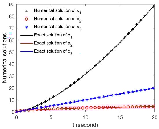
Figure 1. Comparison between the exact solutions and the numerical solutions obtained by the present mothed.

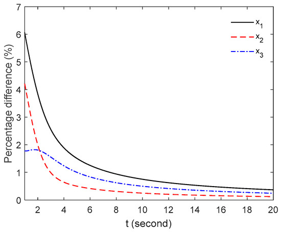
Figure 2. Percentage differences between the exact solutions and the present method.

Next, the effect of time step on the accuracy of the present method is studied. Figure 3, Figure 4 and Figure 5 show the percentage difference between the numerical solutions and the exact solutions for different time steps, h = 0.001, 0.005, 0.01 and 0.02. As shown in the figures, for all cases of time steps, the percentage difference increases when t → 1, but within 5% when 5 < t < 35. For the case of t > 25, the percentage difference increases with the increase in t. Note that for all solutions, the larger the step is, the larger the error is. For the case of t > 35, the accuracy of small step is still good (when h = 0.001, the maximum error at t = 50 is about 1%), while the accuracy of large step drops sharply.

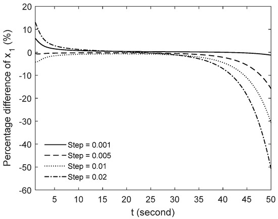
Figure 3. Percentage difference of x₁ between the exact solutions and the present method for different time steps h.

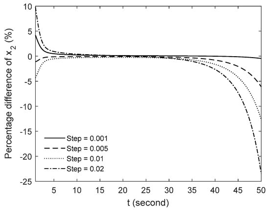
Figure 4. Percentage difference of x₂ between the exact solutions and the present method for different time steps h.

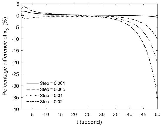
Figure 5. Percentage difference of x₃ between the exact solutions and the present method for different time steps h.

6.2. Comparisons with Other Methods

Chen et al. [26] proposed a numerical method for solving fractional differential equations by using the Grünwald–Letnikov definition. Wang et al. [20] introduced the sliding mode control method to the FDAEs, and obtained the numerical solution by using the predictor-corrector method [23]. In this section, we aim to study the characteristics of the present method by comparing with the two numerical methods.

Consider a numerical example, given by

$$\{\begin{array}{l}{\dot{x}}_1=-x_1+x_2-x_1^{(\alpha )}+x_2{x}_3\\ {\dot{x}}_2=0.5x_1-x_2\\ {\dot{x}}_3=x_1-x_3\\ x_2-x_1{x}_3=0\end{array}$$

(29)

Assume that the initial condition is x(τ) = (1, 1, 1)^T, (τ ≤ 0) and the order of fractional calculus is α = 0.25. According to Equation (1), the above equation can be expressed in matrix form, and hence, the coefficient matrices and the nonlinear part are

$$A=\left[\begin{array}{ccc}-1& 1& 0\\ 0.5& -1& 0\\ 1& 0& -1\end{array}\right],B_1=\left[\begin{array}{ccc}-1& 0& 0\\ 0& 0& 0\\ 0& 0& 0\end{array}\right],f\left(x,t\right)=\left[\begin{array}{c}{x}_2{x}_3\\ 0\\ 0\end{array}\right].$$

(30)

Note that Equation (29) has no external input, hence w(t) = 0 and B₂ = 0. According to the sliding mode theory, we convert Equation (29) into fractional differential equation as Equation (4). The control matrix g(x) should satisfy two conditions as mentioned above, and then we let g(x) = (0, 1, 0)^T. The sliding mode surface is s = x₂ − x_1×3 = 0, and we set the parameters of sliding mode ε = λ = 2.

First, for comparison, we calculate Equation (29) using the numerical method [26], the predictor-corrector method [20] and the present method, respectively. However, the numerical method [26] cannot solve Equation (29) directly, since there is an algebraic equation. Therefore, we convert Equation (29) by substituting the algebraic equation x₂ − x₁x₃ = 0 into the fractional differential equations, and obtain

$$\{\begin{array}{l}{\dot{x}}_1=-x_1-x_1^{(\alpha )}+x_1{x}_3+x_1{x}_3^2\\ {\dot{x}}_3=x_1-x_3\end{array}$$

(31)

The above equations are equivalent to Equation (29) and suitable for the numerical method [26].

Next, we compare the solutions calculated by the numerical method [26], the predictor-corrector method [20] and the present method. Figure 6 shows the numerical results of three methods with the time step h = 0.01. As shown in this figure, the curves of results are not in good agreement when t = 1 to 10. The results of the present method are basically smaller than those of other method. Figure 7 shows the numerical results of three methods with time step h = 0.001. From the figure, the results of three methods are in good agreement for the case of h = 0.001. Therefore, the validity of the present method can be proved. Note that the results of the two methods [20,26] are very close, even for different h. However, Figure 6 and Figure 7 cannot examine the accuracy of the present method since there is no exact solutions for comparison.

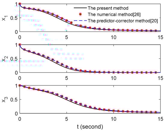
Figure 6. Numerical solutions of x₁, x₂ and x₃ for the case of h = 0.01.

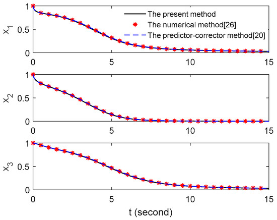
Figure 7. Numerical solutions of x₁, x₂ and x₃ for the case of h = 0.001.

Next, in order to illustrate the accuracy of the present method, we compare its results with those obtained by extremely small step h. Figure 8 shows the relative error of the present method and the numerical method [26] comparing to the solution of the numerical method [26] with h = 0.0001. Because there is no exact solutions for Equation (29), the results calculated by the numerical method [26] with a sufficiently small step (h = 0.0001) are regarded as high-precision solutions. In this section, we only consider the value of x₁ and examine its accuracy. Note that for the both cases of h = 0.01 and 0.001, the present method has higher precision than the numerical method [26].

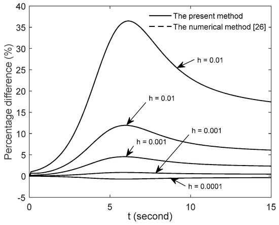
Figure 8. Percentage difference of x₁ obtained by the present method and the numerical method [26] comparing to the numerical method [26] with h = 0.0001.

Table 1 lists the maximum percentage differences of three methods for different steps h. It clearly indicates that the accuracy of the numerical method [26] and the predictor-corrector method [20] is equivalent. However, the present method is much more accurate than the other two methods. For the case of h = 0.001, the maximum percentage difference of the present method is less than 1%, while those of the other methods are about 4.5%. For the case of h = 0.0005, the accuracy of the present method is sufficiently high, and the error is less than 0.07%.

Table 1. The maximum percentage differences for three methods by comparing with the results of the numerical method [26] of h = 0.0001.

No.	Method	Maximum Difference (%)
		h = 0.01	h = 0.001	h = 0.0005	h = 0.0001
1	The numerical method [26]	36.47	4.56	2.31	0
2	The predictor-corrector method [20]	36.94	4.57	2.31	0
3	The present method	11.93	0.85	0.066	−0.70

Table 2 lists the time consumptions of the three methods for different time steps. Note that the numerical method [26] takes the longest time for the same case of h, which is about twice as long as the predictor-corrector method [20]. This illustrates that the computing efficiency is low when solving FDAEs using the numerical method of fractional differential equations. For all cases of h, the predictor-corrector method is the most efficient algorithm, and the present method is very close to it. In fact, the time differences between the two methods can be negligible in most cases. However, according to Table 1, the present method with h = 0.001 is much more accurate than the predictor-corrector method with h = 0.0005. It only takes 1.60 s for the present method to yield solutions with maximum error about 0.85%. From this point of view, the present method is the most efficient one, because it takes the shortest CPU time but obtains the highest precision.

Table 2. Time consumptions of numerical computing for different methods.

No.	Method	CPU Time (s)
		h = 0.01	h = 0.001	h = 0.0005	h = 0.0001
1	The numerical method [26]	0.10	2.23	7.16	190.95
2	The predictor-corrector method [20]	0.05	1.10	3.66	96.16
3	The present method	0.12	1.60	4.36	102.25

6.3. The Effect of Violation Corrections

The violation corrections can extremely improve the accuracy of the present method. In this section, we study the effect of violation corrections on the accuracy of the present method by using the example Equation (29). Additionally, we consider only the value of x₁ for comparison in this section. Figure 9 shows the comparison between the present method with violation correction and that without violation correction for different time steps. As shown in the figure, the percentage difference increases with increasing h. It illustrates that the violation corrections are more effective for large step h. Figure 10 shows the percentage difference of four methods with h = 0.01 comparing to the numerical method [26] with h = 0.0001. As shown in the figure, the present method has the highest precision under such conditions. Moreover, it can be seen that even without violation correction, the accuracy of the present method is higher than that of the other two methods.

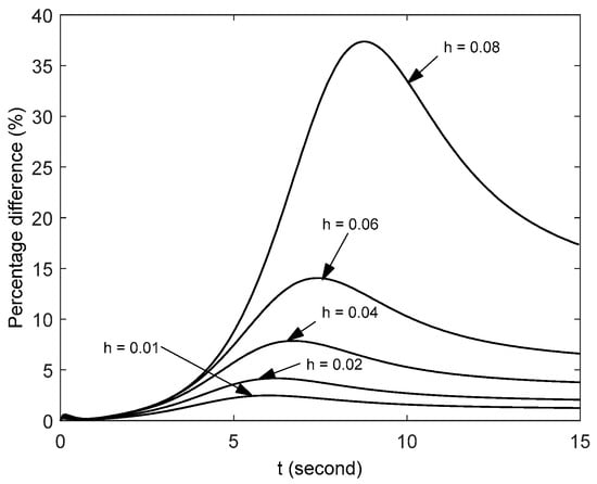
Figure 9. Percentage difference between the present method with violation correction and that without violation correction for different time steps h.

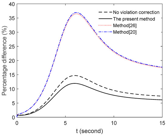
Figure 10. Percentage difference of four methods with h = 0.01 comparing to the numerical method [26] with h = 0.0001.

7. Conclusions

This paper presents a numerical algorithm of FDAEs based on the theory of sliding mode control. The direct violation correction method is used to improve the accuracy of the present method. An example with exact solutions is given to illustrate the validity and precision of the present method. It proves that the solution technology of this paper can be applied in a wide range and possesses a very high accuracy. Additionally, the present method is compared to other two numerical methods. It is found that for the same time step, the present method is more accurate, and its time consumption of computing is close to the fastest method. The effect of violation corrections is investigated for the representative example of FDAEs and is found to be very effective for improving the accuracy of the present method.

References

- Podlubny, I.; Chechkin, A.; Skovranek, T.; Chen, Y.Q.; Jara, B.M.V. Matrix approach to discrete fractional calculus II: Partial fractional differential equations. J. Comput. Phys. 2009, 228, 3137–3153. [Google Scholar] [CrossRef]
- Moshrefi-Torbati, M.; Hammond, J.K. Physical and geometrical interpretation of fractional operators. J. Frankl. Inst. 1998, 335, 1077–1086. [Google Scholar] [CrossRef]
- Xu, J.; Chen, Y.; Tai, Y.; Xu, X.; Shi, G.; Chen, N. Vibration analysis of complex fractional viscoelastic beam structures by the wave method. Int. J. Mech. Sci. 2020, 167, 105204. [Google Scholar] [CrossRef]
- Giona, M.; Cerbelli, S.; Roman, H.E. Fractional diffusion equation and relaxation in complex viscoelastic materials. Phys. A Stat. Mech. Appl. 1992, 191, 449–453. [Google Scholar] [CrossRef]
- Ingman, D.; Suzdalnitsky, J. Application of differential operator with servo-order function in model of viscoelastic deformation process. J. Eng. Mech. 2005, 131, 763–767. [Google Scholar] [CrossRef]
- Povstenko, Y. Fractional heat conduction in a space with a source varying harmonically in time and associated thermal stresses. J. Therm. Stresses 2016, 39, 1442–1450. [Google Scholar] [CrossRef]
- Sun, H.G.; Zhang, Y.; Baleanu, D.; Chen, W.; Chen, Y.Q. A new collection of real world applications of fractional calculus in science and engineering. Commun. Nonlinear Sci. Numer. Simul. 2018, 64, 213–231. [Google Scholar] [CrossRef]
- Podlubny, I. Fractional-order systems and PI/sup /spl lambda//D/sup /spl mu//-controllers. IEEE Trans. Autom. Control 1999, 44, 208–214. [Google Scholar] [CrossRef]
- Vinagre, B.; Petráš, I.; Podlubny, I.; Chen, Y.Q. Using fractional order adjustment rules and fractional order reference models in model-reference adaptive control. Nonlinear Dyn. 2002, 29, 269–279. [Google Scholar] [CrossRef]
- Chen, N.; Tai, Y.; Chen, N. Nonlinear suspension of fractional order calculus in the application of the variable structure sliding mode control. Dyn. Control 2009, 7, 258–263. [Google Scholar]
- Gad, S.; Metered, H.; Bassuiny, A.; Ghany, A.M.A. Multi-objective genetic algorithm fractional-order PID controller for semi-active magnetorheologically damped seat suspension. J. Vib. Control 2017, 23, 1248–1266. [Google Scholar] [CrossRef]
- Mehrmann, V.; Wunderlich, L. Hybrid systems of differential-algebraic equations—Analysis and numerical solution. J. Process. Control 2009, 19, 1218–1228. [Google Scholar] [CrossRef]
- Louca, L.S. Modal analysis reduction of multi-body systems with generic damping. J. Comput. Sci. 2014, 5, 415–426. [Google Scholar] [CrossRef]
- Carpinelli, M.; Gubitosa, M.; Mundo, D.; Desmet, W. Automated independent coordinates’ switching for the solution of stiff DAEs with the linearly implicit Euler method. Multibody Syst. Dyn. 2016, 36, 67–85. [Google Scholar] [CrossRef]
- Ghanbari, F.; Ghanbari, K.; Mokhtary, P. Generalized Jacobi-Galerkin method for nonlinear fractional differential algebraic equations. Comput. Appl. Math. 2018, 37, 5456–5475. [Google Scholar] [CrossRef]
- Ding, X.L.; Jiang, Y.L. Nonnegativity of Solutions of Nonlinear Fractional Differential-Algebraic Equations. Acta Math. Sci. 2018, 38, 756–768. [Google Scholar] [CrossRef]
- Liu, H.; Fu, Y.; Li, B. Discrete Waveform Relaxation Method for Linear Fractional Delay Differential-Algebraic Equations. Discret. Dyn. Nat. Soc. 2017, 2017, 6306570. [Google Scholar] [CrossRef]
- Ghanbari, F.; Mokhtary, P.; Ghanbari, K. Numerical solution of a class of fractional order integro-differential algebraic equations using Muntz-Jacobi Tau method. J. Comput. Appl. Math. 2019, 362, 172–184. [Google Scholar] [CrossRef]
- Ghanbari, F.; Mokhtary, P.; Ghanbari, K. On the numerical solution of a class of linear fractional integro-differential algebraic equations with weakly singular kernels. Appl. Numer. Math. 2019, 144, 1–20. [Google Scholar] [CrossRef]
- Wang, L.; Chen, N. The predictor-corrector solution for fractional order differential algebraic equation. In Proceedings of the 2014 International Conference on Fractional Differentiation and Its Applications (ICFDA 2014), Catania, Italia, 23–25 June 2014; pp. 1–6. [Google Scholar]
- Mortezaee, M.; Ghovatmand, M.; Nazemi, A. Solving variable-order fractional differential algebraic equations via generalized fuzzy hyperbolic model with application in electric circuit modeling. Soft Comput. 2020. [Google Scholar] [CrossRef]
- Ibis, B.; Bayram, M. Numerical comparison of methods for solving fractional differential-algebraic equations (FDAEs). Comput. Math. Appl. 2011, 62, 3270–3278. [Google Scholar] [CrossRef]
- Diethelm, K.; Ford, N.J.; Freed, A.D. A Predictor-Corrector Approach for the Numerical Solution of Fractional Differential Equations. Nonlinear Dyn. 2002, 29, 3–22. [Google Scholar] [CrossRef]
- Podlubny, I. Fractional Differential Equations; ACADEMIC PRESS: San Diego, CA, USA, 1999; p. 198. [Google Scholar]
- Hung, J.Y.; Gao, W.; Hung, J.C. Variable structure control: A survey. IEEE Trans. Ind. Electron. 1993, 40, 2–22. [Google Scholar] [CrossRef]
- Chen, N.; Chen, N.; Tai, Y. A Numerical Scheme for Nonlinear Dynamic System with Fractional Feedback Control. In Proceedings of the ENOC, Rome, Italy, 24–29 July 2011; Volume 7, pp. 24–29. [Google Scholar]
© 2020 by the authors. Licensee MDPI, Basel, Switzerland. This article is an open access article distributed under the terms and conditions of the Creative Commons Attribution (CC BY) license (http://creativecommons.org/licenses/by/4.0/).