Article

The Influences of Asymmetric Market Information on the Dynamics of Duopoly Game

1
Department of Statistics and Operations Research, College of Science, King Saud University, Riyadh 11451, Saudi Arabia
2
Department of Mathematics, Faculty of Science, Mansoura University, Mansoura 35516, Egypt
Mathematics 2020, 8(7), 1132; https://doi.org/10.3390/math8071132
Submission received: 29 June 2020 / Revised: 8 July 2020 / Accepted: 9 July 2020 / Published: 10 July 2020
(This article belongs to the Special Issue Mathematical Analysis in Economics and Management)

Abstract

:
We investigate the complex dynamic characteristics of a duopoly game whose players adopt a gradient-based mechanism to update their outputs and one of them possesses in some way certain information about his/her opponent. We show that knowing such asymmetric information does not give any advantages but affects the stability of the game’s equilibrium points. Theoretically, we prove that the equilibrium points can be destabilized through Neimark-Sacker followed by flip bifurcation. Numerically, we prove that the map describing the game is noninvertible and gives rise to several stable attractors (multistability). Furthermore, the dynamics of the map give different shapes of quite complicated attraction basins of periodic cycles.

1. Introduction

The Duopoly game has been increasingly studied in the literature because of the complex dynamic characteristics it possesses. Different kinds of this game arise based on the strategies adopted by its players (or firms). These strategies may be quantities (Cournot game) or prices (Bertrand game). In this paper, we deal with a quantity-based duopoly game. Because of the nature of competition among the players and the information available in the market players in such games have used different types of adjustment mechanisms in order to update their output productions. There are some popular adjustment mechanisms that have been reported in the literature such as the bounded rationality which is a gradient-based mechanism. In such mechanism players carry out estimation about their profits whether they increase or decrease in order to increase or decrease their productions in the next period of time. An intensive information about this mechanism has been reported in the literature [1,2,3,4,5,6]. Other reported adjustment mechanisms in the literature include naive mechanism, local monopolistic approximation (LMA) mechanism, and the tit-for-tat approach. All of those mechanisms have reported important dynamic characteristics of such games and have led different types of bifurcations that make the game’s equilibria be destabilized due to chaos. The routes to chaos in these games are because of Neimark-Sacker and flip bifurcations. In this introduction, we give some reported contributions on the complex dynamic characteristics of such games. There is no doubt that Puu with his work [1] opened the way to several studies in this research direction. He introduced a Cournot duopoly game whose players adopt prices derived from an isoelastic demand function obtained from the utility function of Cobb-Douglas. Puu analyzed the stability conditions of the game’s equilibrium and concluded that it has become unstable due to flip bifurcation. In [7], a simple adjustment process has been adopted by competed firms in an economic market problem. The adjustment process depended on the current amount sold versus prices in previous time. Elsadany [8] has analyzed the complex dynamics of a Cournot duopoly game whose players updated their outputs productions based on some estimation on the relative profits. The local monopolistic approximation approach has been applied by Cavalli et al. [9] on a duopoly game with quantities setting. They have proved that the game had a converging Nash point due to the adoption of such approach. In [10], Ahmed et al. have introduced a multi-team duopoly game with quantities setting and have investigated the stability conditions of the game’s equilibrium points. In [11], the authors studied a game of triopoly whose players are heterogeneous and their demand functions are isoelastic. Other important studied have been reported in the literature such as the works by, Zhang et al. [12], Ma et al. [13], Peng et al. [14], Tramontana et al. [15], Leonard and Nishimura [16], Askar [17], Ahmed et al. [18], Peng et al. [19], and Askar et al. [20].
The current paper follows the research direction of duopoly games whose players adopt gradient-based mechanism but one player knows some information about its competitor. The asymmetry of information possessed by one player about the other is important in microeconomics. This kind of information has not been applied for economic games whose players use gradient-based mechanism such as bounded rationality. The paper introduces a rich analysis of the dynamic characteristics of such games such as stability attractors(multistability) and basin of attractions. It generalizes the work studied in [21] however the model discussed in [21] may have a missing parameter which may affect the analysis done there. Our main results which are the core of this paper concentrate on the stability of the equilibrium points and especially on the stability of the interior equilibrium point. We show that the asymmetric information possessed by one player about the other affects the stabilization behavior of the equilibrium point. For different set of parameters’ values we show that the region of stability of each player in 1D bifurcation diagram is the same for both player even though the second player has known some information about his/her competitor. Instead different types of quite complicated attraction basins are emerged for some periodic cycles. Furthermore, the analysis performed about the map describing the game shows that the map is noninvertible and this may the main reason for rising quite complicated basin of attractions.
Now we summarize the parts of the paper as follows. In Section 2, we introduce the model describing the game discussed in this paper. Section 3 is divided into three parts which are the main results in the paper. The first part calculates the equilibria of the game and investigates their stability. The second part discusses the local and global analysis of the dynamic behavior of the game’s map via numerical simulation. The last part calculates the critical curves of the map and discusses its invertibility. The last section concludes the obtained results.

2. The Model

The market structure we assume here consists of two competed players (or firms). Such competition between two players is known in the literature as a duopoly game. Both firms advertise differentiated products in the market so that they attract consumers who are focusing on such kind of products. The outputs of both firms are quantities produced by each firm and are denoted by q 1 and q 2 . Indeed, each firm wants to achieve its optimum of production and this is accomplished by maximizing their profits as follows.
M a x q i π i ( q i , q i ) = q i p i C i ( q i )
where q i refers to the omitted component. Since the products are differentiated then they adopt different prices. To achieve different prices we recall the utility function suggested by Singh and Vives [22]. It takes the following form,
U ( q 1 , q 2 ) = a ( q 1 + q 2 ) 1 2 ( q 1 2 + q 2 2 + 2 b q 1 q 2 ) ; q 1 , q 2 > 0
This utility has some important properties that are:
  • It is a concave function 2 U q i 2 = 1 < 0 ; i = 1 , 2 that means the marginal utility of each good is decreasing.
  • The marginal utility of good 1 is not independent of good 2. This means 2 U q 1 q 2 = b 0 .
  • It is not homogeneous, U ( θ q 1 , θ q 2 ) θ U ( q 1 , q 2 ) . It means that utility rises by a scalar if each good is multiplied by the same scalar.
  • Under the budget constraint i = 1 2 p i q i m we have the following maximization problem,
M a x U ( q 1 , q 2 ) s . t i = 1 2 p i q i m
where m is a constant and p i is the price of good i. Solving (3) gives the following inverse demand functions.
p 1 = a q 1 b q 2 , p 2 = a q 2 b q 1
where a is a constant price in case market is not supported by quantities. The parameter b has some advantages. It refers to a degree of horizontal differentiation. Taking b = 0 yields a market that is dominated by two monopoly firms. While b = 1 we get two identical firms with less differentiated products. Negative values for this parameter achieve complementarity between the firms and hence we restrict it on the interval ( 1 , 1 ) . Assuming that both firms adopt linear costs, C i ( q i ) = c q i where c refers to a constant marginal cost. Using (4) with this cost we have the profit of each firm as follows.
π 1 = ( a c q 1 b q 2 ) q 1 , π 2 = ( a c q 2 b q 1 ) q 2
Now each firm wants to detect its optimum output to get a maximized profit. This occurs at q ¯ 1 , q ¯ 2 which is obtained at setting π i q i = 0 , i = 1 , 2 as follows.
π 1 q 1 = a c 2 q 1 b q 2 = 0 π 2 q 2 = a c 2 q 2 b q 1 = 0
Solving (6) gives q ¯ 1 , q ¯ 2 = a c 2 + b , a c 2 + b which is positive provided that a > c . We consider now two bounded rational players who adjust their production at discrete time step based on a gradient-based mechanism given by,
q 1 ( t + 1 ) = q 1 ( t ) + k q 1 ( t ) π 1 ( q 1 ( t ) , q 2 ( t ) ) q 1 , q 2 ( t + 1 ) = q 2 ( t ) + k q 2 ( t ) π 2 ( q 1 ( t + 1 ) , q 2 ( t ) ) q 2
The second equation in (7) reveals that the second player knows the quantity produced by the first firm at time t + 1 . This kind of asymmetric information changes the second equation in (7) as follows. Substituting (6) in (7) gives the discrete dynamical map that describes the game at hand.
T q 1 , q 2 : q 1 ( t + 1 ) = q 1 ( t ) + k q 1 ( t ) a c 2 q 1 ( t ) b q 2 ( t ) , q 2 ( t + 1 ) = q 2 ( t ) + k q 2 ( t ) a c 2 q 2 ( t ) b q 1 ( t ) b k 2 q 1 ( t ) q 2 ( t ) a c 2 q 1 ( t ) b q 2 ( t )
The next section gives rise to the complex dynamic characteristics of the map (8). This includes the routes making the map’s fixed points get destabilized.

3. Main Results

3.1. Fixed Points and Stability

The map (8) admits the following fixed points:
E 0 = ( 0 , 0 ) , E 1 = 0 , a c 2 , E 2 = a c 2 , 0 , E 3 = a c b + 2 , a c b + 2
The first three points are called corner points and the last one corresponds to the Nash equilibrium point. They are all positive provided that a > c . The local stability of these points is governed by calculating the Jacobian matrix of the map (8) as follows.
J m = J 11 J 12 J 21 J 22
where
J 11 = 1 + k a c 4 q 1 b q 2 , J 12 = b k q 1 , J 21 = k b q 2 b k 2 q 2 a c 2 q 1 b q 2 + 2 b k 2 q 1 q 2 , J 22 = 1 + k a c 4 q 2 b q 1 + 2 b 2 q 1 q 2 a b q 1 + b c q 1 + 2 b q 1 2 k 2
The trace τ and determinant δ of the Jacobian (9) are,
τ = 2 + k 2 ( a c ) ( 4 + b ) q 1 ( 4 + b ) q 2 b k 2 q 1 a c ( 1 + b ) q 2 2 q 1 , δ = 1 k a c + b q 2 4 q 1 1 + k ( a c b q 1 4 q 2 ) b q 1 k 2 ( a c b q 2 2 q 1 )
The map (8) is characterized according to the following cases:
  • If δ < 1 it is a dissipative map,
  • If δ = 1 it is a conservative map,
  • Otherwise it is called an undissipative map.
In addition, the local stability of any fixed point q ¯ 1 , q ¯ 2 depends on the eigenvalues λ 1 and λ 2 of the Jacobian (9) as follows.
  • If λ 1 , 2 < 1 the fixed point q ¯ 1 , q ¯ 2 is locally asymptotically stable and is called an attracting node.
  • If λ 1 , 2 > 1 the fixed point q ¯ 1 , q ¯ 2 is unstable repelling node.
  • If λ 1 < 1 and λ 2 > 1 (or λ 1 > 1 and λ 2 < 1 ) the fixed point q ¯ 1 , q ¯ 2 is a saddle point.
  • If λ 1 = 1 and λ 2 1 (or λ 1 1 and λ 2 = 1 ) the fixed point q ¯ 1 , q ¯ 2 is a non-hyperbolic point.
Proposition 1.
The fixed point E 0 is an unstable repelling point.
Proof. 
The Jacobian at this point has two equal real eigenvalues, λ 1 , 2 = 1 + k ( a c ) that have λ 1 , 2 > 1 . This completes the proof. □
Proposition 2.
Both E 1 and E 2 are unstable saddle points.
Proof. 
The Jacobian at the point E 1 has two equal real eigenvalues, λ 1 = 1 k ( a c ) and λ 2 = 1 + k 2 ( a c ) ( 2 b ) . Since we have a > c and b < 1 we get λ 1 < 1 and λ 2 > 1 and then E 1 is unstable saddle fixed point. The same proof is for E 2 . □
Proposition 3.
The fixed point E 3 is locally asymptotically stable provided that k < 2 + b a c .
Proof. 
The Jacobian at this point becomes
J m = 1 2 A k b A k b A k ( 2 A k 1 ) 1 2 A k + A 2 b 2 k 2
where A = a c 2 + b . The trace and determinant of J m become,
τ = 2 4 A k + A 2 b 2 k 2 , δ = ( 1 2 A k ) 2
Now we have,
1 τ + δ = ( 2 + b ) ( 2 b ) A 2 k 2 , 1 + τ + δ = 4 ( 1 A k ) 2 + A 2 b 2 k 2 , 1 δ = 4 A k ( 1 A k )
It clear that 1 τ + δ > 0 is always satisfied and 1 δ > 0 if k < 2 + b a c . □
Proposition 4.
The fixed point E 3 is unstable due to Neimark-Sacker bifurcation only if k > 2 + b a c .
Proof. 
It is clear that 1 δ < 0 if k > 2 + b a c . □

3.2. Local and Global Analysis via Numerical Simulation

In this subsection, we study the impact of the parameter k on the dynamics of map (8) as it is selected to be the bifurcation parameter. We start our numerical simulation by setting the following parameters set, a = 0.7 , b = 0.3 , k = 3.8 and c = 0.1 with the initial datum ( q 1 , q 2 ) = ( 0.11 , 0.12 ) . As this set, the fixed point E 3 = 0.2608695652 , 0.2608695652 and the Jacobian becomes,
J m = 0.98261 0.29739 0.29222 0.89417
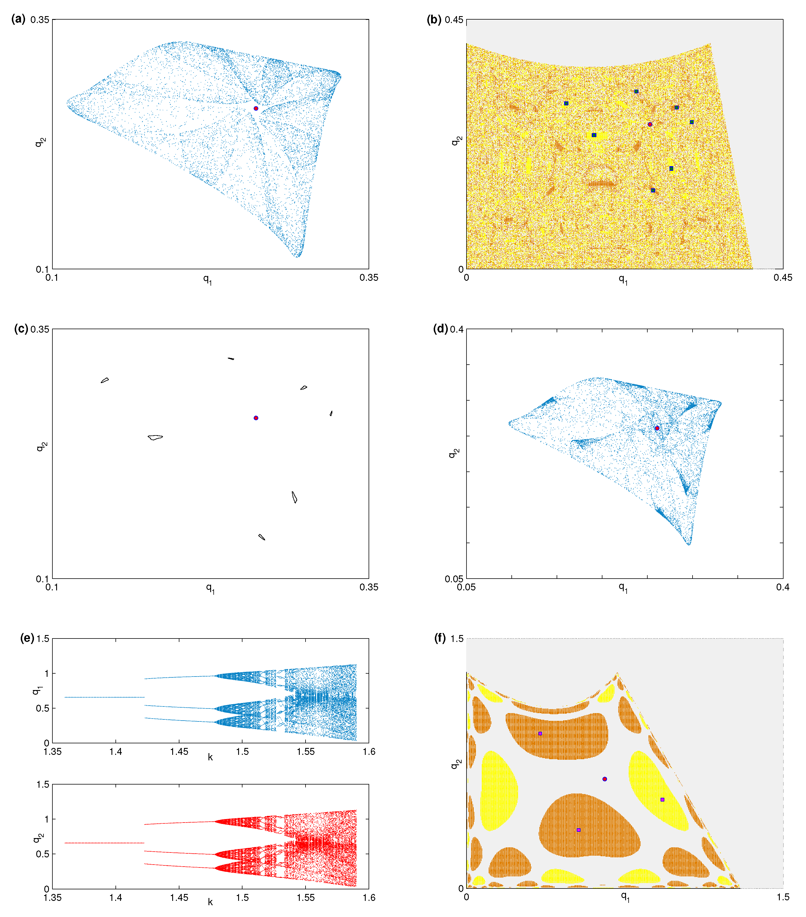
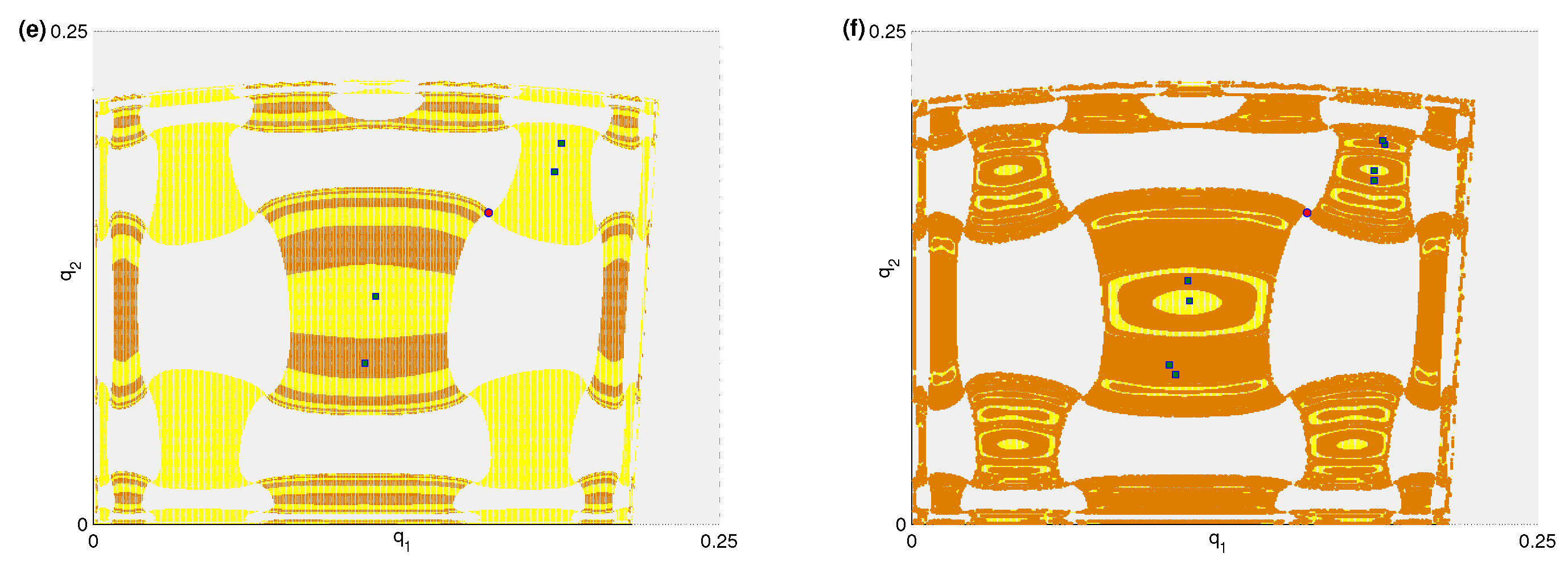
with two complex eigenvalues, λ 1 , 2 = 0.93839 ± 0.29146 i whose modulus, λ 1 , 2 = 0.98261 . Simple calculations show that the stability triangle at E 3 , S = 1 τ + δ > 0 , 1 + τ + δ > 0 , 1 δ > 0 is satisfied. This means that the fixed point E 3 is locally asymptotically stable. As the bifurcation parameter k increases the fixed point E 3 can be destabilized because of the coexistence of Neimark-Sacker bifurcation. Figure 1a displays that the fixed point becomes stable for all k until k approaches 3.8 on where a Neimark-Sacker bifurcation takes place and then it gets unstable. Increasing k above 3.8 gives rise to closed invariant curves. For example, Figure 1b,c depict different dynamical situations around the fixed point represented by red circle. They show spirals that are changed in closed invariant curves then closed rings at different values of the parameter k as written top of each figure. The other parameters’ values are keep fixed. Increasing k to 4.4 and keeping the other parameters’ values fixed a period-9 cycle is emerged. It has a complicated attraction basin as plotted in Figure 1d. This cycle is denoted by squares in the figure with orange and yellow colors while the grey color denotes divergent and infeasible points. Increasing k to 4.45 a period-18 cycle is born with a quite complicated attraction basin as shown in Figure 1e. Further increasing in k results in a complicated chaotic attractor around the fixed point. This chaotic attractor is given in Figure 1f and it continues to occur as k increases further until it becomes more complicated at k = 4.59 as depicted in Figure 2a. The chaotic behavior then turns into a period-7 cycle with more complicated basin of attraction as given in Figure 2b. It is born at k = 4.6436 with the other parameters fixed. Further increase in the bifurcation parameter k gives rise to a seven closed chaotic areas plotted in Figure 2c. They are coexisted at k = 4.6 and the other parameters’ values are fixed. Any other increase results in a one piece of chaotic attractor as shown in Figure 2d which is plotted at k = 4.66 . Now, we assume another set of parameters’ values, a = 2 , b = 0.9 , c = 0.1 . It assumes high values for a and b keeping the marginal cost low. This set presents a different dynamic situation for the map (8). At this set, E 3 = 0.6551724138 , 0.6551724138 and the Jacobian becomes,
J m = 0.86069 0.83731 0.72066 0.15960
with two complex eigenvalues, λ 1 , 2 = 0.51014 ± 0.69321 i whose modulus, λ 1 , 2 = 0.86069 . It is easy to see that the stability triangle at E 3 is satisfied. This means that the fixed point E 3 is locally asymptotically stable. Figure 2e shows that the fixed point gets unstable due to Neimark-Sacker bifurcation starting to appear after three discontinuous period-3 cycle. The period-3 cycle is displayed in Figure 2f with its attraction basin at k = 1.43 . As in the previous attraction basins, the grey color denotes the divergent and infeasible points while the other two colors refer to the period-3 basin. Increasing k to 1.4 9 gives rise to three closed invariant curves as plotted in Figure 3a. These closed curves become larger as k increases until k reaches 1.516 on where a period-15 is emerged. Its attraction basin that is quite complicated is given in Figure 2b at k = 1.516 . At k = 1.525 the dynamic situation is converted into three closed rings as shown in Figure 3c. A complicated basin of attraction for a period-18 cycle is displayed in Figure 3d at k = 1.5288 . Any further increase in k gives more complicated attractors for the map (8). In Figure 3e,f we display two complex chaotic attractors for the map at k = 1.558 and k = 1.59 , respectively.
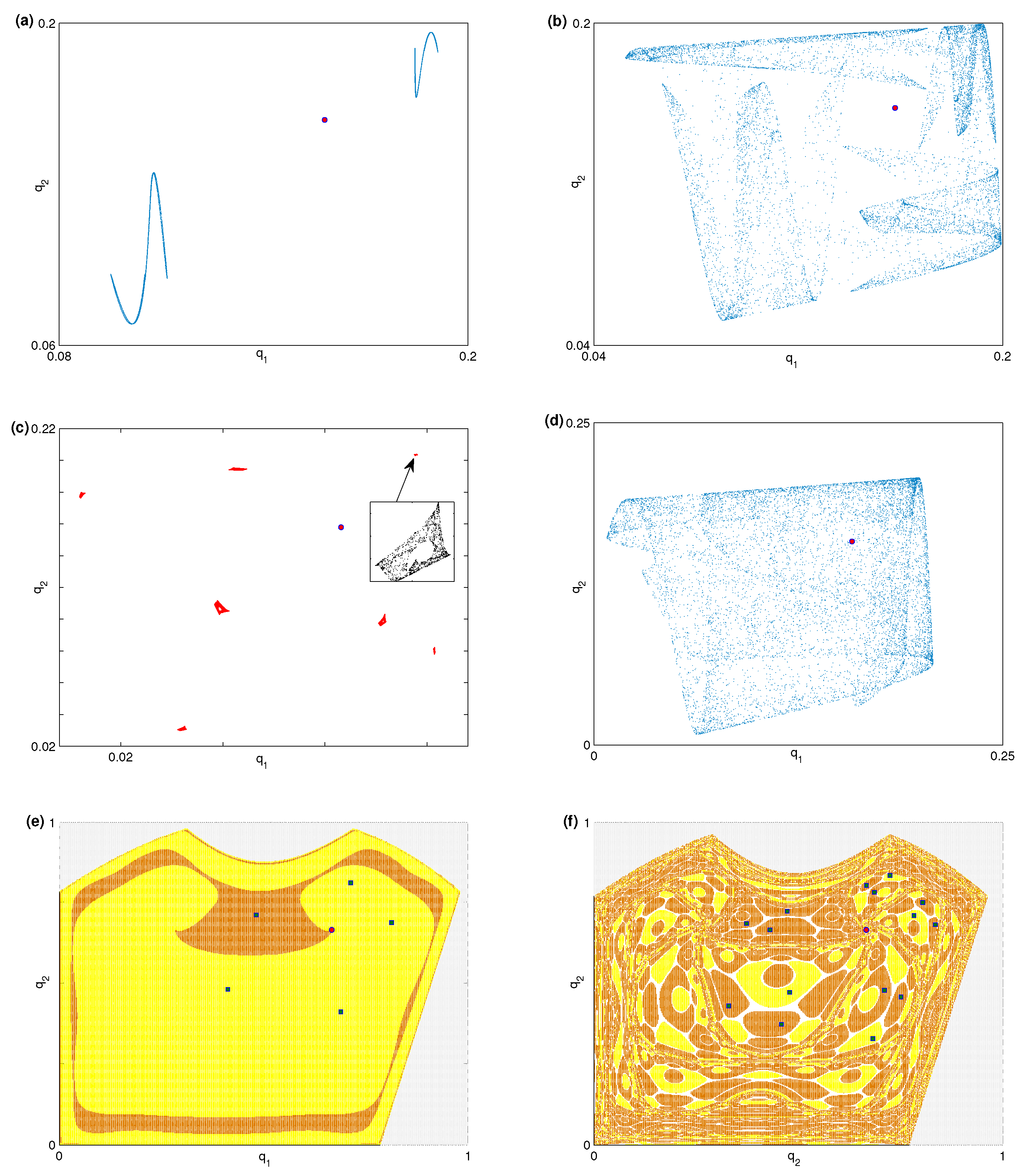
There is another set of parameters’ values that gives interesting dynamic characteristics for the map (8). In this set, we assume high marginal cost c with high constant price a and with negative value for b. We assume the following set, a = 2.3 , b = 0.1 and c = 2 . At this set, E 3 = 0.157894737 , 0157894737 becomes locally stable for all the values of k until k = 6.33 on where a spiral around it arises. Using this set of parameters’ values gives rise to a Neimark-Sacker that is followed by a flip bifurcation as k increases. Figure 4 and Figure 5 show different dynamic situations for the map at this set.

3.3. Critical Curves and Noninvertibility

The obtained results on the basin of attraction show that it is quite complicated due to some periodic cycles. Such structure of the attraction basin makes us to investigate some features of the map such as critical curves and noninvertibility property. Setting q 1 , t + 1 = q ´ 1 and q 2 , t + 1 = q ´ 2 in the map (8) where indicates time evolution we get,
T : q ´ 1 = q 1 + k q 1 a c 2 q 1 b q 2 , q ´ 2 = q 2 + k q 2 ( a c 2 q 2 b q 1 ) b k 2 q 1 q 2 a c 2 q 1 b q 2
Let ( q ´ 1 , q ´ 2 ) R and solving algebraically the map (12) with respect to q 1 and q 2 , we get 0 , 2 and 4 real rank-1 preimages. For simplicity, we assume the following, a = 0.7 , c = 0.1 , b = 0.3 , k = 4.59 , q ´ 1 = 0 and solving algebraically the map (12) we get,
q 1 + = 0.37826 + 4.5 × 10 15 4.6452 × 10 25 1.2104 × 10 26 q ´ 2 , q 1 = 0.37826 4.5 × 10 15 4.6452 × 10 25 1.2104 × 10 26 q ´ 2
and then we have,
q 2 + = 0.071077 + 0.016340 q ´ 2 1.0428 × 10 14 4.6452 × 10 25 1.2104 × 10 26 q ´ 2 0.37826 + 4.5 × 10 15 4.6452 × 10 25 1.2104 × 10 26 q ´ 2 , q 2 = 0.071077 + 0.016340 q ´ 2 + 1.0428 × 10 14 4.6452 × 10 25 1.2104 × 10 26 q ´ 2 0.37826 4.5 × 10 15 4.6452 × 10 25 1.2104 × 10 26 q ´ 2
This means we have two real preimages q 1 + , q 2 + and q 1 , q 2 if q ´ 2 < 0.38377 and hence we are in zone Z 2 in the phase plane, otherwise we do not have real preimages and in this case we are in zone Z 0 . On the other hand, we assume a = 0.7 , c = 0.1 , b = 0.3 , k = 4.59 , q ´ 2 = 0 and solving algebraically the map (12) gives,
q 1 + , 1 = 0.20447 ± 1.10893 × 10 4 3.5231 × 10 6 9.18 × 10 6 q ´ 1 , q 1 + + , 1 = 0.011250 q ´ 1 + 0.17380 ± 0.27233 × 10 5 1.7065 × 10 7 q ´ 1 1.4161 × 10 10 q ´ 1 + 4.0727 × 10 9 )
and then we have,
q 2 + , 2 = 1.4892 × 10 5 0.32825 × 10 4 q ´ 1 5.4742 × 10 6 3.5231 9.18 q ´ 1 0.20447 ± 0.10893 3.5231 9.18 q ´ 1 , q 2 + + , 2 = 0.071076 0.021462 q ´ 1 0.0016875 q ´ 1 2 ± 1.1135 0.40849 q ´ 1 × 10 3 × 17.065 q ´ 1 2 + 14161 q ´ 1 + 4072.7 0.17380 + 0.011250 q ´ 1 0.27233 × 10 2 × 17.065 q ´ 1 2 + 14161 q ´ 1 + 4072.7
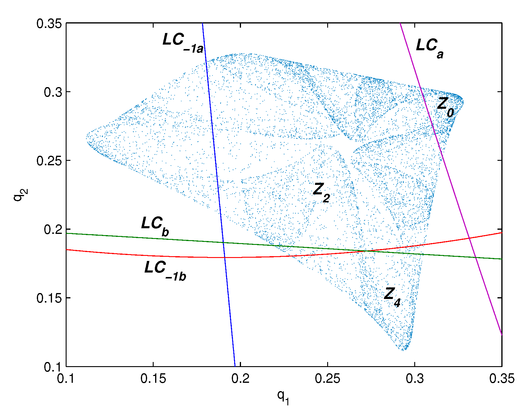
This means we have four real preimages q 1 + , q 2 + , q 1 , q 2 , q 1 + + , q 2 + + and q 1 , q 2 provided that q ´ 1 < 0.28771 and then we are in zone Z 4 . If 0.28771 < q ´ 1 < 0.38377 we have only two real preimages which means we are in zone Z 2 . If q ´ 1 > 0.38377 we have no preimages and so we are in Z 0 . This concludes that the map is noninvertible and the phase plane of the map (12) may be divided into three zones that are Z 0 , Z 2 and Z 4 . Since we have three zones we have to get the critical curves that separate those zones. To calculate the critical curve L C we evaluate L C 1 first by putting δ = 0 ,
1 k a c + b q 2 4 q 1 1 + k ( a c b q 1 4 q 2 ) b q 1 k 2 ( a c b q 2 2 q 1 ) = 0
So we have L C 1 = L C 1 a L C 1 b where,
L C 1 a : q 1 = 1 + k ( a c b q 2 ) k b L C 1 b : q 2 = 1 + k ( a c b q 1 ) b k 2 ( a c 2 q 1 ) q 1 k ( 4 k b 2 q 1 )
Then the critical curve L C = T ( L C 1 ) can be written as L C = L C a L C b where,
L C a : q 1 = 1 8 k b k q 2 + k ( a c ) 1 3 b k q 2 + k ( a c ) + 3 , L C b : q 2 = 2 1 k ( a c b q 1 ) b k 2 ( a c 2 q 1 ) q 1 2 k ( 4 k b 2 q 1 ) 2
In Figure 6 we plot both L C and L C 1 at the parameters’ values, a = 0.7 , c = 0.1 , b = 0.3 , k = 4.59 . It is obvious that L C separates the phase plane into three zones as discussed above.

4. Conclusions

A duopoly game whose players have asymmetric information about each other has been modelled and studied. The equilibrium points of this game have been calculated and their stability conditions have been discussed. The discussion has shown that the asymmetric information does not have any advantages for the player who adopted but it affects the stability of game. It has been analyzed that the interior equilibrium point of the game can be destabilized due to the coexistence of Neimark-Sacker directly followed by flip bifurcation. Our obtained results have investigated the occurrence of quite complicated basin of attractions for high periodic cycles. We have shown the appearance of different types of complicated basins for the map described the game at different sets of parameters’ values. Furthermore, we have analyzed the phase plane of the map that has been divided into three zones, Z 0 , Z 2 and Z 4 which are formed due to the nonlinear and noninvertible game’s map. The obtained results in this paper are rich and generalize some work in the literature [21]; however the model discussed in [21] has a missing parameter which may affect the analysis carried out in that paper. Our future contributions to develop such research direction are to study the influences of asymmetric information on the dynamic behavior of games whose players are heterogenous. Indeed, this also requires to study its effects on triopoly games with different heuristics.

Funding

Research Supporting Project number (RSP-2020/167), King Suad University, Riyadh, Saudi Arabia.

Acknowledgments

Research Supporting Project number (RSP-2020/167), King Suad University, Riyadh, Saudi Arabia.

Conflicts of Interest

The authors declare no conflict of interest.

References

  1. Puu, T. Chaos in duopoly pricing. Chaos Solitons Fractals 1991, 1, 573–581. [Google Scholar] [CrossRef]
  2. Askar, S.S.; Al-khedhairi, A. Dynamic investigations in a duopoly game with price competition based on relative profit and profit maximization. J. Comput. Appl. Math. 2020, 367, 112464. [Google Scholar] [CrossRef]
  3. Naimzada, A.K.; Raimondo, R. Chaotic congestion games. Applied Math. Comput. 2018, 321, 333–348. [Google Scholar] [CrossRef]
  4. Askar, S.S.; Al-khedhairi, A. On complex dynamic investigations of a piecewise smooth nonlinear duopoly game. Chaos Solitons Fractals 2020, 139, 110001. [Google Scholar] [CrossRef]
  5. Askar, S.S.; Al-khedhairi, A. The dynamics of a business game: A 2D-piecewise smooth nonlinear map. Phys. A Stat. Mech. Its Appl. 2020, 537, 122766. [Google Scholar] [CrossRef]
  6. Ma, J.; Sun, L.; Hou, S.; Zhan, X. Complexity study on the Cournot-Bertrand mixed duopoly game model with market share preference. Chaos 2018, 28, 023101-10. [Google Scholar] [CrossRef] [PubMed]
  7. Tuinstra, J. A price adjustment process in a model of monopolistic competition. Int. Game Theory Rev. 2004, 6, 417–442. [Google Scholar] [CrossRef]
  8. Elsadany, A.A. Dynamics of a Cournot duopoly game with bounded rationality based on relative profit maximization. Appl. Math. Comput. 2017, 294, 253–263. [Google Scholar] [CrossRef]
  9. Cavalli, F.; Naimzada, A.; Tramontana, F. Nonlinear dynamics and global analysis of a heterogeneous Cournot duopoly with a local monopolistic approach versus a gradient rule with endogenous reactivity. Commun. Nonlinear Sci. Numer. Simul. 2015, 23, 245–262. [Google Scholar] [CrossRef] [Green Version]
  10. Ahmed, E.; Hegazi, A.S.; Elettreby, M.F.; Askar, S.S. On multi-team games. Phys. A Stat. Mech. Its Appl. 2006, 369, 809–816. [Google Scholar] [CrossRef]
  11. Tramontana, F. Heterogeneous duopoly with isoelastic demand function. Econ. Model. 2010, 27, 350–357. [Google Scholar] [CrossRef]
  12. Zhang, J.; Da, Q.; Wang, Y. Analysis of nonlinear duopoly game with heterogeneous players. Econ. Model. 2007, 24, 138–148. [Google Scholar] [CrossRef]
  13. Ma, J.; Si, F. Complex Dynamics of a Continuous Bertrand Duopoly Game Model with Two-Stage Delay. Entropy 2016, 18, 266. [Google Scholar] [CrossRef]
  14. Peng, Y.; Lu, Q. Complex dynamics analysis for a duopoly Stackelberg game model with bounded rationality. Appl. Math. Comput. 2015, 271, 259–268. [Google Scholar] [CrossRef]
  15. Tramontana, F.; Elsadany, A.E.A. Heterogeneous triopoly game with isoelastic demand function. Nonlinear Dyn. 2012, 68, 187–193. [Google Scholar] [CrossRef]
  16. Leonard, D.; Nishimura, K. Nonlinear dynamics in the Cournot model without information. Ann. Oper. Res. 1999, 89, 165–173. [Google Scholar] [CrossRef]
  17. Askar, S.S. Tripoly Stackelberg game model: One leader versus two followers. Appl. Math. Comput. 2018, 328, 301–311. [Google Scholar] [CrossRef]
  18. Ahmed, E.; Elettreby, M.F. Controls of the complex dynamics of a multi-market Cournot model. Econ. Model. 2014, 37, 251–254. [Google Scholar] [CrossRef]
  19. Peng, J.; Miao, Z.; Zheng, L. Study on dynamical properties and simulation of a four-dimensional nonlinear discrete dynamics. In Proceedings of the 2011 IEEE International Conference on Industrial Engineering and Engineering Management, Singapore, 6–9 December 2011. [Google Scholar] [CrossRef]
  20. Askar, S.S.; Alnowibet, K. Nonlinear oligopolistic game with isoelastic demand function: Rationality and local monopolistic approximation. Chaos Solitons Fractals 2016, 84, 15–22. [Google Scholar] [CrossRef]
  21. Ueda, M. Effect of information asymmetry in Cournot duopoly game with bounded rationality. Appl. Math. Comput. 2019, 362, 124535. [Google Scholar] [CrossRef] [Green Version]
  22. Singh, N.; Vives, X. Price and quantity competition in a differentiated duopoly. Rand J. Econ. 1984, 15, 546–554. [Google Scholar] [CrossRef]
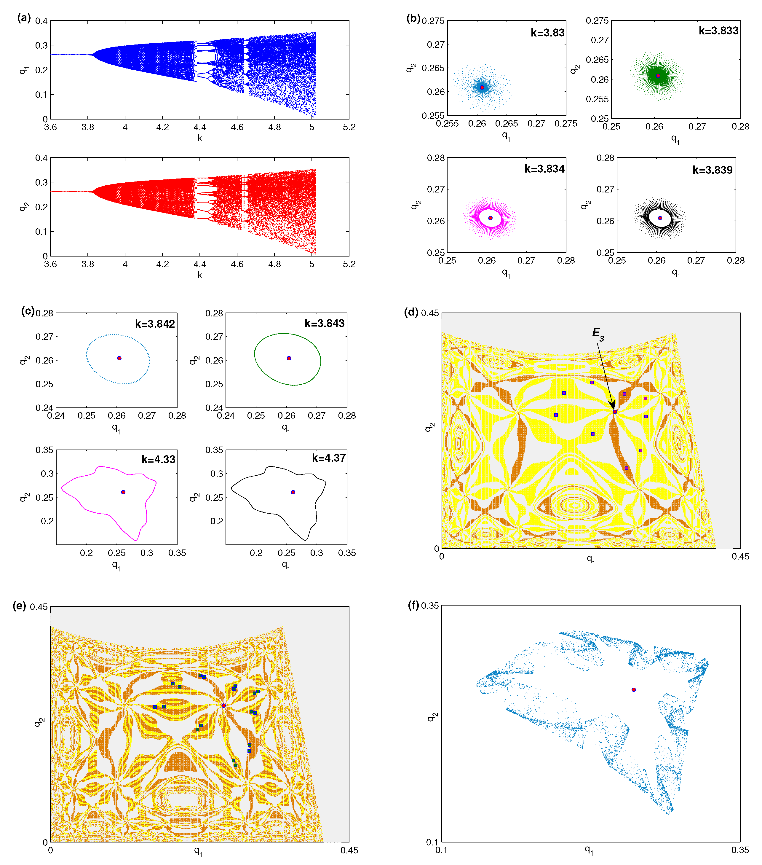
Figure 1. (a) Neimark-Sacker bifurcation on varying k. (b,c) Different dynamical situations at different values of k. (d) The basin of attraction of the period-9 cycle at k = 4.4 . (e) The basin of attraction of the period-18 cycle at k = 4.45 . (f) Chaotic attractor at k = 4.50 . The other parameters’ values are, a = 0.7 , b = 0.3 and c = 0.1 with the initial datum ( q 1 , q 2 ) = ( 0.11 , 0.12 ) .
Mathematics 08 01132 g001
Figure 2. (a) The phase plane of the chaotic attractor at k = 4.59 . (b) The basin of attraction of period-7 cycle at k = 4.6436 . (c) The phase plane of seven closed chaotic areas at k = 4.65 . (d) The phase plane of the chaotic attractor at k = 4.66 . (e) Neimark-Sacker bifurcation on varying k and a = 2 , b = 0.9 , c = 0.1 . (f) The basin of attraction of the period-3 cycle at k = 1.43 and a = 2 , b = 0.9 , c = 0.1 .
Mathematics 08 01132 g002
Figure 3. (a) The phase plane of three closed invariant curves at k = 1.49 . (b) Basin of attraction of period-15 cycle at k = 1.516 . (c) The phase plane of three closed chaotic areas at k = 1.525 . (d) Basin of attraction of period-18 cycle at k = 1.5288 . (e) The phase plane of a chaotic attractor at k = 1.558 . (f) The phase plane of a chaotic attractor at k = 1.59 . Other parameters’ values are a = 2 , b = 0.9 , c = 0.1 .
Mathematics 08 01132 g003aMathematics 08 01132 g003b
Figure 4. (a) Neimark-Sacker bifurcation on varying k. (b) Spiral and closed invariant curves at different values of k. (c) The phase plane of a chaotic attractor at k = 7.23 . (d) The basin of attraction of period-2 cycle at k = 7.43 . (e) The basin of attraction of period-4 cycle at k = 7.66 . (f) The basin of attraction of period-8 cycle at k = 7.77 .
Mathematics 08 01132 g004aMathematics 08 01132 g004b
Figure 5. (a) The phase plane of two unconnected chaotic attractors at k = 7.9 . (b) The phase plane of a chaotic attractor at k = 8.2 . (c) The phase plane of seven unconnected chaotic attractors at k = 8.566 . (d) The phase plane of a chaotic attractor at k = 8.86 . (e) The basin of attraction of period-5 cycle at k = 1.75 . (f) The basin of attraction of period-15 cycle at k = 1.98 . The data set is a = 2.3 , b = 0.1 and c = 2 for (ad). The data set is a = 2 , b = 0.5 and c = 1 for (e,f).
Mathematics 08 01132 g005
Figure 6. The critical curves at the parameters’ values a = 0.7 , c = 0.1 , b = 0.3 and k = 4.59 .
Mathematics 08 01132 g006