A Highly Efficient Neural Network Solution for Automated Detection of Pointer Meters with Different Analog Scales Operating in Different Conditions

Abstract

We investigate a neural network–based solution for the Automatic Meter Reading detection problem, applied to analog dial gauges. We employ a convolutional neural network with a non-linear Network in Network kernel. Presently, there is a significant interest in systems for automatic detection of analog dial gauges, particularly in the energy and household sectors, but the problem is not yet sufficiently addressed in research. Our method is a universal three-level model that takes an image as an input and outputs circular bounding areas, object classes, grids of reference points for all symbols on the front panel of the device and positions of display pointers. Since all analog pointer meters have a common nature, this multi-cascade model can serve various types of devices if its capacity is sufficient. The model is using global regression for locations of symbols, which provides resilient results even for low image quality and overlapping symbols. In this work, we do not focus on the pointer location detection since it heavily depends on the shape of the pointer. We prepare training data and benchmark the algorithm with our own framework a3net, not relying on third-party neural network solutions. The experimental results demonstrate the versatility of the proposed methods, high accuracy, and resilience of reference points detection.

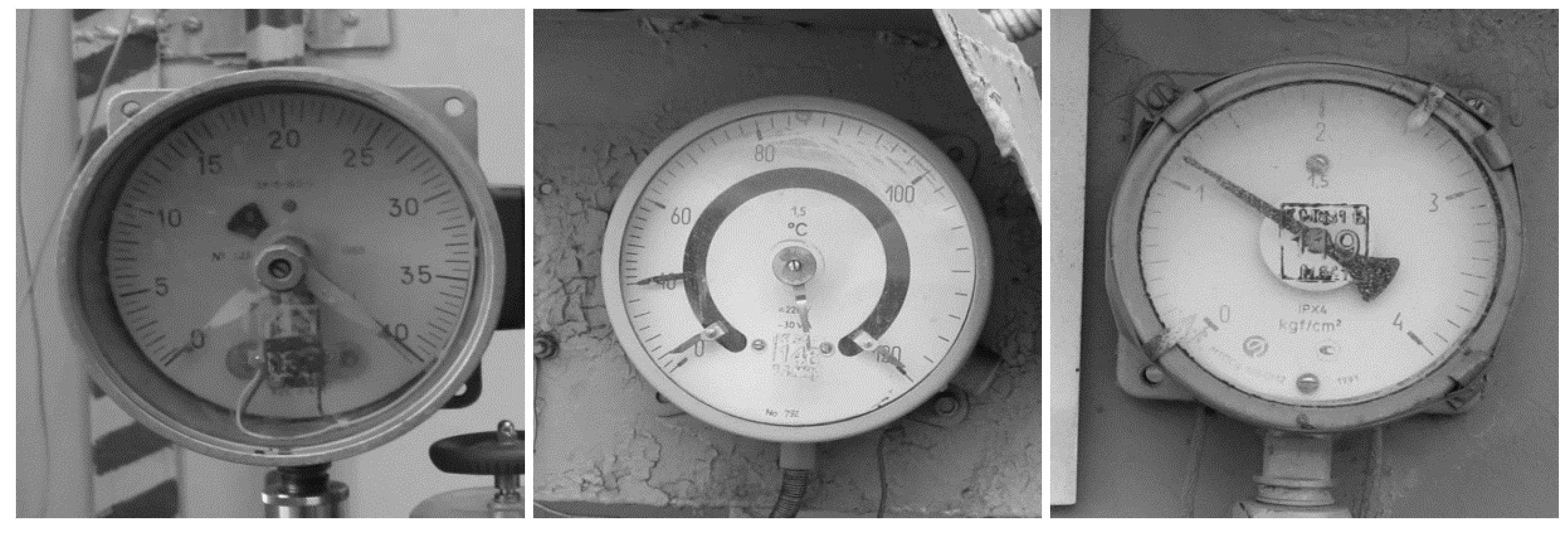
1. Introduction

Recent successes in object detection with convolutional neural networks (CNNs) suggest an opportunity to employ them for analog dial gauges detection (Figure 1). Dial gauges are analog measurement devices with pointers indicating the measured quality with its position. There are a great many objects that come with pointer meters, some of critical importance for safety. Often, such meters can not be simply replaced by a digital device and that requires a means of automated reading from the analog meters. This work aims not only to solve the problem but also to explore the abilities of neural networks to achieve resilient object detection for complex objects composed of simple parts. Specifically, analog dial gauges are comprised of dials, pointers and symbols. The achievements of this work could be translated to other types of objects, for example when a regressive generation of a grid of reference points is needed for facial landmark detection [1,2].

Resilient generation of an object’s grid is also important for other problems and in this work we describe our procedures for training data preparation; the structure of the neural networks, which are combined in a cascade; and the training procedure. The main interests in object detection for analog dial gauges are similar to any other automatic meter readings: automated data acquisition; elimination of a human factor for reading data; and elimination of the risk factors for reading data from dangerous cites, such as power plants.

Our experience in looking for datasets for this problem is similar to Gabriel Salomon et al. [3]—we were not able to find suitable datasets of meaningful volume. The dataset in Reference [3] is small and too specific and also does not have labels for reference symbols, that is why we prepare a dataset ourselves. The dataset is created from real data, acquired during the process of automation of a power plant. The particularly important for the success of the solution choices are convolutional neural networks with non-linear convolution kernels and unit-initialization.

There is a variety of object detection solutions today. Regarding objects for automatic meter reading, most works look at reading data from gauges with cyclometer and electronic displays. When detection produces correct results, the readings are virtually perfectly accurate. This is not the case for analog pointer meters, for which it is essentially impossible to produce precise readings. That can explain the lack of research for reading from analog dial gauges, particularly via neural networks.

In Reference [4], the image processing procedure is divided into four steps including image preprocessing, target region positioning, character segmentation and character recognition. Only for this last step, the authors use a neural network. Even though the authors work with a dataset that has images with variations of viewing angles, scale and lighting, this method does not produce sufficiently resilient results since the segmentation of indiscriminate symbols on an image does not produce accurate output.

Bao et al. [5] work with inverse perspective mapping, binarization and Hough transformation method to align the image of a meter improving the pointer location detection. However, the research does not mention complex images and also the suggested method for training data preparation seems excessively labor-intensive.

The same can be said about the approach from Reference [6], also employing binarization and Hough transformation. In Reference [7], SURF method was utilized to match with a template image and then Hough transformation was used to detect the pointer.

In Reference [8], a neural network works as the first cascade for meter localization. Fang et al. [9] suggest to use the neural network Mask R-CNN [10] for key points detection; we follow the idea of using a neural network for key points detection, however, our implementation is different.

Zuo et al. [11] also use Mast R-CNN but prefer PrRoIPooling over RoiAlign. The work is focusing on the pointer detection and localization while the position of the meter is assumed fixed, which reduces the applicability of the method in a real-world environment. The authors present a community dataset for testing, but we were not able to get access to it since their publication is rather recent, however, this is not a very significant issue since our dataset appears to be competitive to it and also presents data acquired in a real-world environment, not in a lab.

Gabriel Salomon et al. [3] compute bounding boxes of pointer meter dials via the neural network-based methods YOLO [12] and Faster-RCNN [13]. However, in their work, they do not detect key points for symbols.

Most of the listed methods are tied to specific devices limiting their general applicability. It is important to point out that the presented analysis seems to suggest that neural network-based methods are superior to traditional image processing methods. Most of the modern neural network-based methods in this field rely on convolutional (CNN) networks [14,15], for example, detectors [12,13,16,17,18,19]. There are variations in the number of layers and filters, the sizes of filters, the choices of hyperparameters, and the methods of optimization.

A standard CNN has a set of standard linear filters with an $k\in {\mathbb{R}}^{M,M}$ kernel. Increasing the stride induces interlacing, which reduces the accuracy of the output. Pooling, required to reduce the dimensions of the network, has a negative impact on the preservation of the spacial information about the objects and spacial information is key for the regression of the coordinates of the objects. Another factor is residual blocks [20] which are often accompany neural network-solutions, but the presence of such blocks is commonly implemented by assemblies of shallow networks [21], which in turn limits the capacity C of the network [22].

To set the scope of this work more clearly, it is important to point out that the aim is not to recognize symbols, recognition of symbols is needed in the case of local detection. But with global detection, the aim is to localize the whole grid of symbols centers on the face of the device simultaneously. So, if even a few symbols would not be recognizable at all, the algorithm should still have good chances to detect centers of symbols correctly. And this is one of the main ideas of the approach; to do it globally. As for symbols recognition—it is possible to identify symbols exclusively by matching them with a template that was provided beforehand for each type of device. First, the type of the device must be detected (to select the proper template), and after that global regression is performed and, finally, the template is matched to the symbols.

2. Materials and Methods

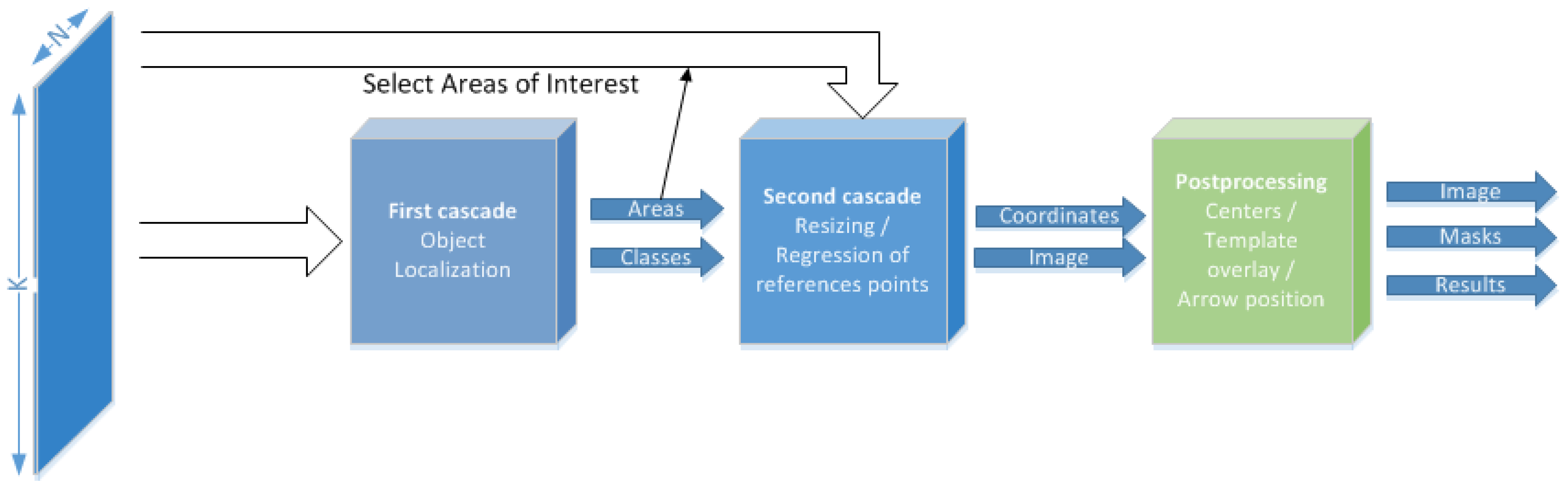
2.1. AMR Detector

The suggested architecture contains non-linear classifiers type NiN [23,24,25], more specifically the solution a3net [26], which follows a particular approach to identitying matrix initialization for building a deep network [27]. The initialization of the identity matrix occurs at the start of the process with the weight (including the weights for the unitary diagonal) changing during the training process. This procedure, similar to ResNet [20], builds an assembly of shallow networks [21], but later, due to the partial destruction of the unitary connections, it transforms into a monolithic structure efficiently utilizing the capacity C of the network. An example of a typical neural network–based solution is illustrated in Figure 2.

In our particular case we do not use transposed convolution. Also, even for deep-architectures we do not use skip-connections. Non-linear classifiers perform exceptionally well for preserving spacial information until the final convolution layers comparing to linear classifiers with pooling, commonly used in CNN, and at the same time, larger stride allows, in spite of the use of the non-linear kernel, to improve performance for the same degree of the capacity C of the neural network [28].

The detector is comprised of three cascades (Figure 3). The first cascade, traditionally for multi-cascade systems, performs localization of the sought-for objects and cropping the areas of interest. No additional preprocessing, for example brightness histogram balancing, is performed.

The second cascade normalizes the sizes of the cropping areas and performs regression of the coordinates of the key points for the centers of the symbols. In this case, a global optimization regression is chosen. The global regression for all key points produces more resilient results for each symbol’s coordinates localization and key points grid generation even when some of the symbols are indiscriminate or even non-observable. The first two cascades are built as multi-level deep convolutional neural networks with non-linear convolution kernels.

The third cascade computes the position of the pointer. It was rather difficult to prepare training data for this task, so, instead of a neural network, we employed a set of different contrast–correlation–based methods. Here, we do not describe the internal composition of the third cascade and methods for the pointer’s position determination since it can vary from case to case and also because we are mostly interested in the generation of a grid of the key points for the symbols.

2.1.1. Localization of the Objects

The composition of the neural network for three types of devices and base gray images 512 × 512 is listed in

Table 1. Composition of the neural network for localization of objects.

Layer Type	Window/Step/Output	Kernel	Number of Parameters
Conv1	$2\times 2$ / $2\times 2$ / $LRelu$	$4\times 4\times 4$	125
Conv2	$2\times 2$ / $2\times 2$ / $LRelu$	$8\times 8\times 8$	729
Conv3	$2\times 2$ / $2\times 2$ / $LRelu$	$16\times 16\times 16$	4913
Conv4	$2\times 2$ / $2\times 2$ / $LRelu$	$32\times 32\times 32$	36 K
Conv5	$2\times 2$ / $2\times 2$ / $LRelu$	$64\times 64\times 64$	275 K
Conv6	$2\times 2$ / $2\times 2$ / $LRelu$	$128\times 128\times 128$	2.1 M
Conv7	$2\times 2$ / $2\times 2$ / $LRelu$	$256\times 256\times 256$	17 M
Conv8	$2\times 2$ / $2\times 2$ / $LRelu$	$512\times 512\times 512$	135 M
Conv9	$2\times 2$ / $1\times 1$ / $LRelu$	$512\times 512\times 1536$	406 M
Total	−	−	560 M

. The neural network outputs 256 coordinate reference points RP (a rectangle of 16 × 16 points), represented by sets $\{x_0,y_0,d,N_{classes}\}$, where $N_{classes}=3$.

In training and detection, a square grid of coordinate reference points (RP) is overlaid across the input image of any size uniformly and a zero-point is selected randomly. The determination of the center is done by a regression of points, located within a circle with radius r from the center of the device; see Figure 4 where RPs are the blue points and the device centers are green.

The Figure 5 shows a grid of reference points (similar to anchors in well-known detection algorithms) and the result of their convergence to the center of the object. The points marked in gray are inactive agents and do not used further since the object is not included in their activation area, which in turn is determined by some given radius. In the work, it was defined as $\sqrt{{(x_i-x_{i+1})}^2+{(y_i-y_{i+1})}^2}$, where $x_i$ and $y_i$ are coordinates of points in the reference grid.

The reference points are evenly spread in a checkerboard pattern in the center of the detection area. If placed in a regular grid, then a situation may arise when an object, located between the other two objects close together, might be skipped.

Most often, neural network–based detectors work with bounding boxes (BB), not RP, and filtration after detection is executed by non-max suppression (NMS) algorithm. In our case, since we prefer RP instead of BB, for filtering and selection of corrected values we use iterative clustering mean-shift [29] with the tolerance set empirically.

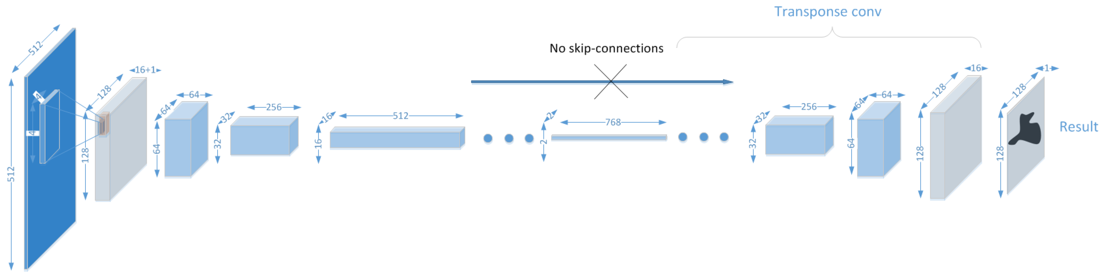
2.1.2. Resizing Cropped Images

After detection of the regions of the meters the algorithm performs resizing of the selected areas of images to the uniform size—a square with side length U = 256 (see Figure 6). This operation significantly simplifies calculations for symbols’ reference points.

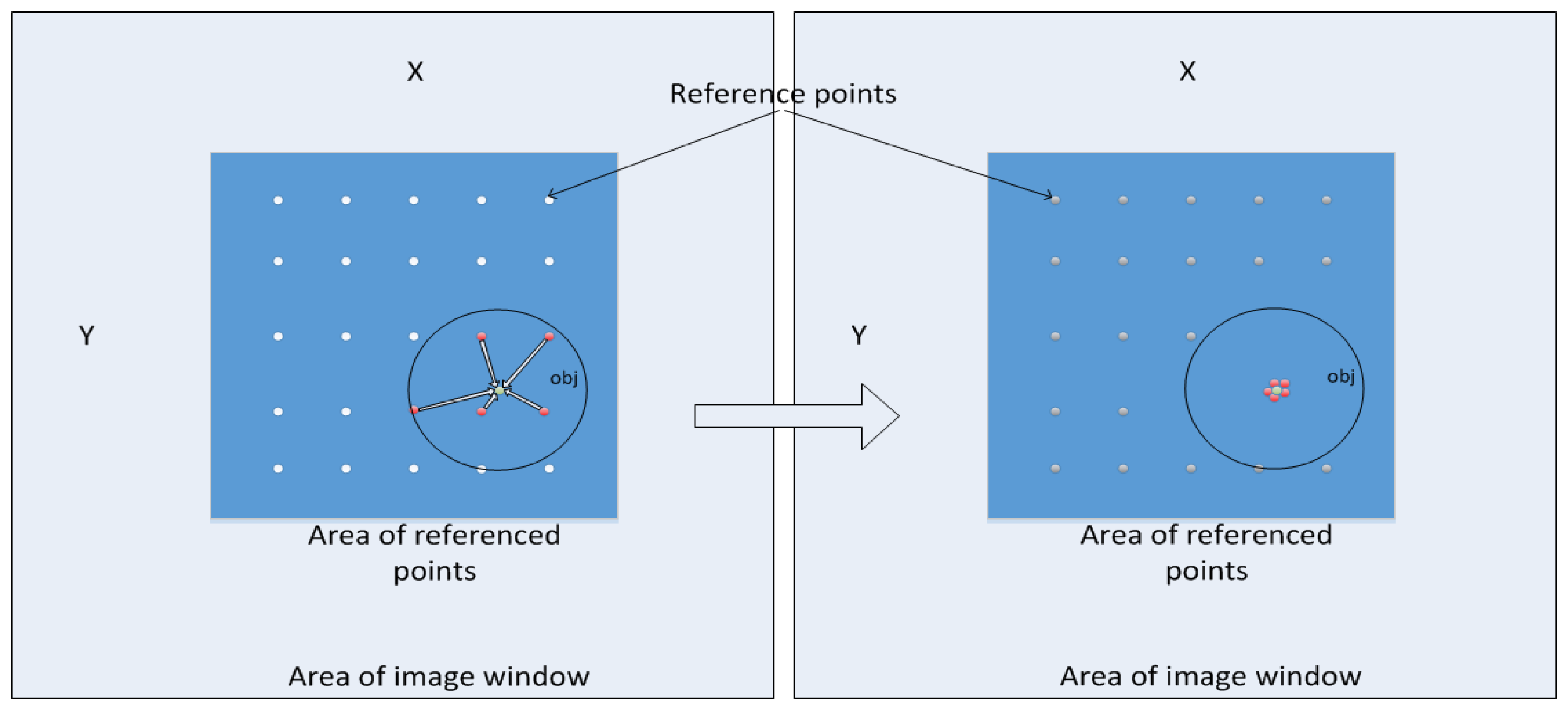
2.1.3. Regression of the Grid of Reference Points

The composition of the neural network for three types of devices and base gray images 256 × 256 is listed in

Table 2. Composition of the neural network for regression of a grid of reference points

Layer Type	Window / Step / Output	Kernel	Number of Parameters
Conv1	$2\times 2$ / $2\times 2$ / $LRelu$	$4\times 4\times 4$	125
Conv2	$2\times 2$ / $2\times 2$ / $LRelu$	$16\times 16\times 16$	4913
Conv3	$2\times 2$ / $2\times 2$ / $LRelu$	$64\times 64\times 64$	275 K
Conv4	$2\times 2$ / $2\times 2$ / $LRelu$	$256\times 256\times 256$	17 M
Conv5	$2\times 2$ / $2\times 2$ / $LRelu$	$256\times 256\times 256$	17 M
Conv6	$2\times 2$ / $2\times 2$ / $LRelu$	$256\times 256\times 256$	17 M
Conv7	$2\times 2$ / $2\times 2$ / $LRelu$	$256\times 256\times 256$	17 M
Conv8	$2\times 2$ / $1\times 1$ / $LRelu$	$256\times 256\times 18$	1.2 M
Total	−	−	70 M

. The network outputs $MA{X}_{pointers}$ reference points with coordinates $\{x0,y0\}$, where $MA{X}_{pointers}$ is determined by the number of symbols (9 in the demonstrated example). The number of output reference points is determined by the type of the device and so localization of the symbols is performed globally for each type.

2.1.4. Characteristics of the Network

To accelerate the training time we use ADAM optimizer ([30]). The batch is 32 and the initial learning rate is 0.0001, decreasing to 0.000001 by the 100th epoch. Initialization of weight is as following:

$$w_{ij}=0.00001\sqrt[2]{\frac{2}{N_{l-1}}}N(\mu ,{\sigma }^2).$$

(1)

The main diagonal is initialized as ${w_1}_{ii}=\lambda$ for each i, where $\lambda$ –> 1, as in [27]. This allows building efficiently trained deep neural network architectures (see also Section 2.1).

The non-linear activation function for all layers is leaky relu:

$$f\left(x\right)=\left\{\begin{array}{cc}x& \mathrm{if}x>0\\ 0.01x& \mathrm{if}x\le 0\end{array}\right.$$

(2)

That allows us to decrease the impact of vanishing gradient and reduce the requirements for computation resources. The error-function is based on MSE (Mean squared error) ${(y-t)}^m$, where $m=3$:

$$L_j\left(i\right)=\frac{1}{3}{(y_j\left(i\right)-t_j\left(i\right))}^2|y_j\left(i\right)-t_j\left(i\right)|{\alpha }_j=C_j{\alpha }_j,$$

(3)

and the derivative:

$$(y_j\left(i\right)-t_j\left(i\right))|y_j\left(i\right)-t_j\left(i\right)|{\alpha }_j,$$

(4)

where L is the current loss for the class j at the i-th iteration, C is the current error for the class j at the i-th iteration, ${\alpha }_j$ is a relaxation coefficient for the class j, $y_j\left(i\right)$ is the output value of the sample i for the class j, and $t_j\left(i\right)$ is the target value of the sample i for the class j.

This type of curve allows, similar to the Focal Loss algorithm [17], to decrease the impact of the less meaningful, but very frequent background class, and to increase the impact of the target class. The same applies to the regression of coordinates.

The complete loss function (Equation (5)) is calculated for all RP at classification and only for the active RP at regression. Active RP meaning the points, attached to the nearest objects on the image, in our case: to the center of the device for the first cascade and to the centers of the symbols for the second cascade.

$$L(\left\{p_{all}\right\},\left\{coor{d}_{all}\right\})=\sum _{i=0}^{N_{boxes}}({\alpha }_p{L}_{cls}(p_i,\stackrel{*}{{c_i}_{0,1}})+\stackrel{*}{{c_i}_{0,1}}{\alpha }_x{L_{reg}}_x{(x_i-\stackrel{*}{x_i})}^2+\stackrel{*}{{c_i}_{0,1}}{\alpha }_y{L_{reg}}_y{(y_i-\stackrel{*}{y_i})}^2),$$

(5)

where the i is the index of a RP, $p_i$ is a predicted probability that the RP is associated with the center of the object, $c_i^{*}$ is a label for positive (1) or negative (0) RP, $L_{cls}$ is the classification loss, and $L_{reg}$ is the regression error.

2.2. Preparation of Training Data

All images for training only have brightness components without any color information. To simplify the labeling of symbols, required to create a dataset, we suggest three methods, each intended to accelerate the preparation.

2.2.1. Labeling and Preparation of the Dataset

The first approach is based on the recurrence and similarity of devices’ images. That allows to only label each N-th image in a row. Specifically, in 10,000 images we only have to label 300–500 before training the network and the rest of the images were labeled later. Typically, following the after-labeling, the remaining non-labeled symbols numbered no more than 5% of the total. Incorrectly labeled images were removed. The architecture of the neural network for the preparation of the dataset is the same as for the detection.

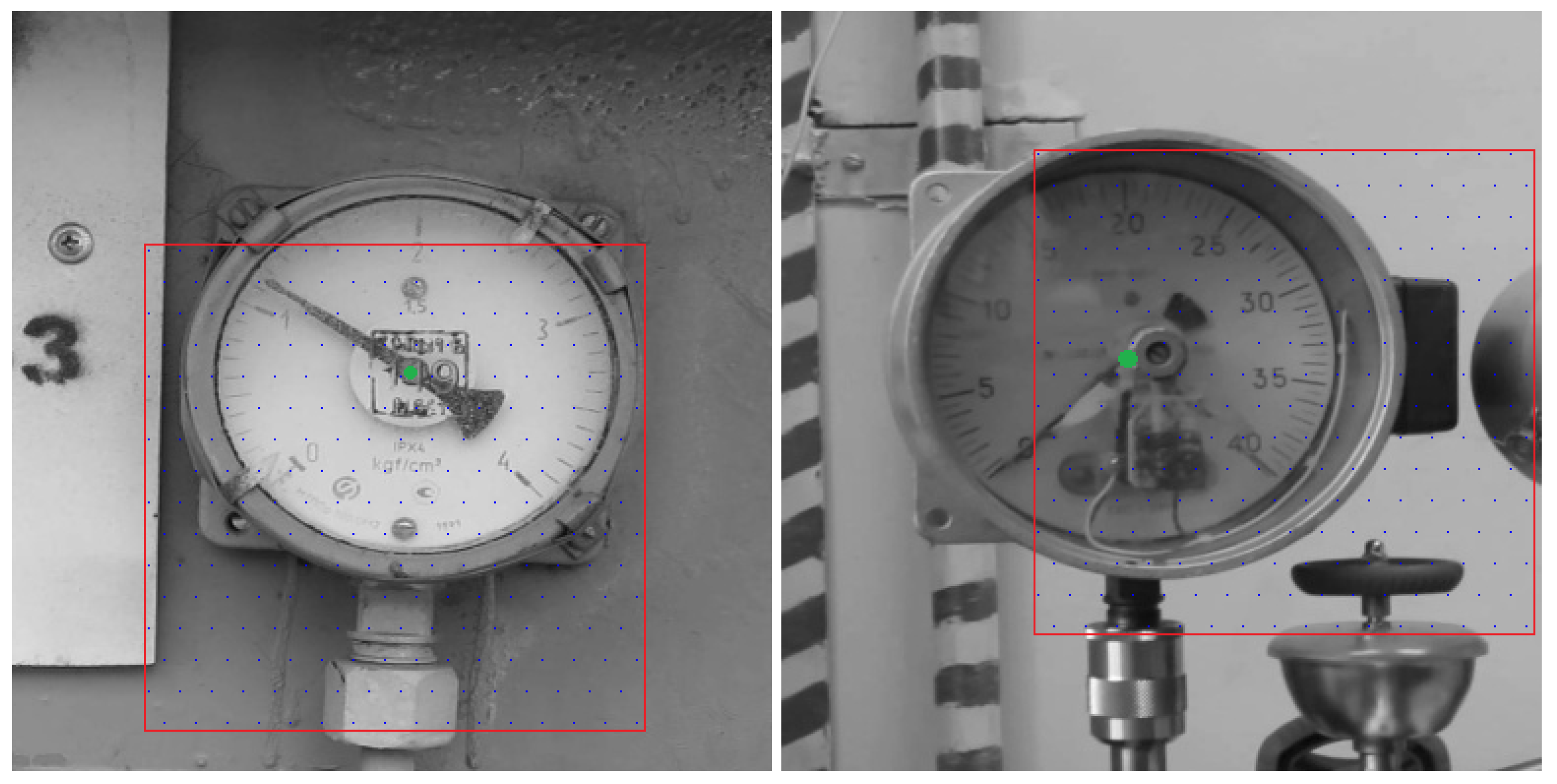
2.2.2. Localization of the Centers of the Devices

The second method computes the centers of the devices and that assists detection. For this approach we assume that symbols are placed approximately in a circle, but not uniformly. To find the center of the circle we use iterative gradient descent. Since the convergence function is not convex, to limit it to a convex segment we set initial coordinates roughly within an imaginary circle. The coordinates of the center can be approximately calculated as a mean $C={\sum }_i\left(S_i\right)$ of the sum of all coordinates of all symbols, where C are the coordinates of the center and $S_i$ are the coordinates of the symbol i. Next, for each pair of radiuses from the current center we calculate a sum of squares of pairwise differences. Keeping in mind the equation of a circle $R^2={(X0-X)}^2+{(Y0-Y)}^2$, the correction function for coordinates is:

$$X{0}_{n+1}=X{0}_n-\alpha {\nabla }_{x}Jx$$

(6)

$$Y{0}_{n+1}=Y{0}_n-\alpha {\nabla }_{y}Jy,$$

(7)

where

$$Jx=\sum _i\left({(({(x0-x1)}^2+{(y0-y1)}^2)-({(x0-x2)}^2+{(y0-y2)}^2))}^2\right)$$

(8)

$$Jy=\sum _i\left({(({(x0-x1)}^2+{(y0-y1)}^2)-({(x0-x2)}^2+{(y0-y2)}^2))}^2\right)$$

(9)

the total sum of differences between each pair of distances, and $\alpha$ is 0.00000000005. Accordingly, the equations with derivatives are:

$$X{0}_{n+1}=X{0}_n-\alpha \sum _i(-4(x1-x2)(-2x0(x1-x2)+x{1}^2-x{2}^2-2y0y1+2y0y2+y{1}^2-y{2}^2))$$

(10)

$$Y{0}_{n+1}=Y{0}_n-\alpha \sum _i(-4(y1-y2)(-2y0(y1-y2)+y{1}^2-y{2}^2-2x0x1+2x0x2+x{1}^2-x{2}^2)).$$

(11)

Expressions (10) and (11) are evaluated until convergence achieved. When the devices have a more pronounced elliptical shape, it might be possible to use the ellipses fitting algorithm [31]. The automated calculation, comparing to manual labeling, allows for more accurate and fast detection of the centers and fewer errors.

2.2.3. Enumeration of the Symbols

The third method relies on the fact that the arc between the first and the last symbol is the longest. This fact enables labeling of symbols after the center of the device is found. This approach for automated matching of symbols to reference points significantly simplifies labeling of symbols. An operator is only required to mark the centers of symbols on an image and the enumeration is then automatically acquired my matching to the type of the device.

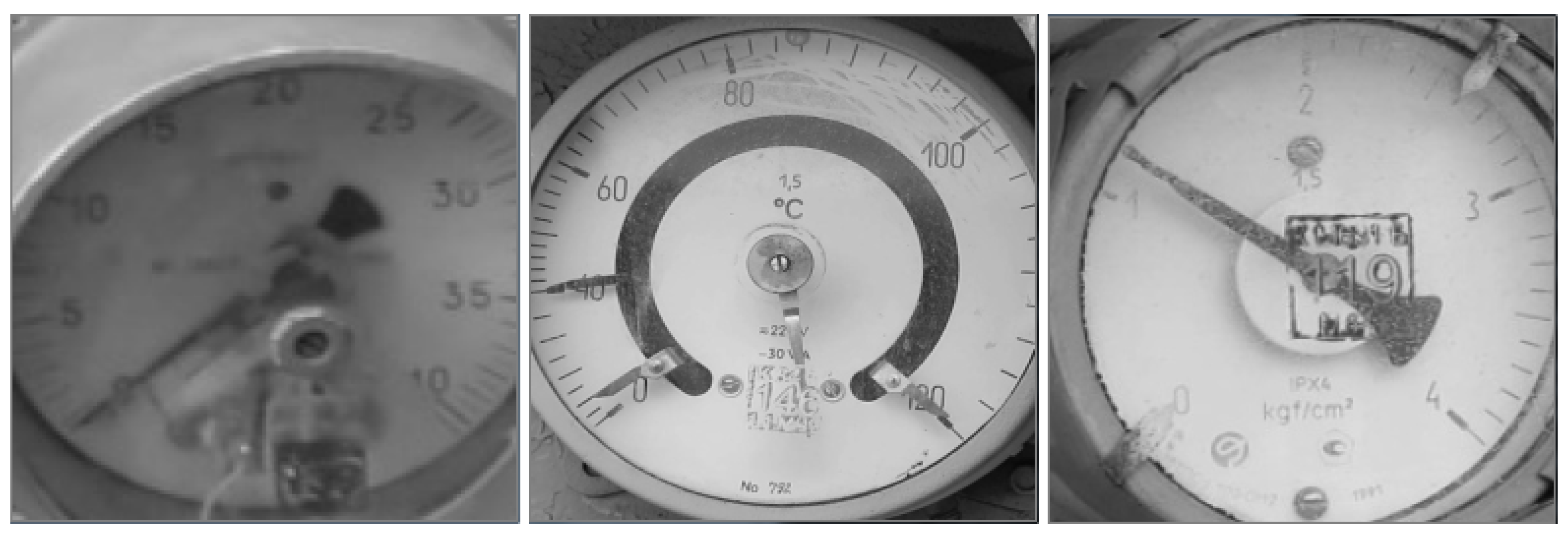
2.3. Experiments

We tested our algorithms and applications on a PC with Intel(R) Xeon(R) E5-2658 v3 CPU @ 2.20 GHz, RAM 32 GB. The programming code was optimized for matrix calculations with SSE2 and GPU. The training was performed with GPU NVIDIA GEFORCE GTX1080 TI 11 GB GDDR5x. We performed testing with the a3net framework [26]. Full detection of the two used in the work cascades on average took about 3 ms for a gray image of 1024 × 512 size.

2.3.1. Type of Device Detection

The goal of the detection is to find sets $\{x_0,y_0,d,N_{classes}\}$, where $N_{classes}=3$. For the 10,000 images each type of device was correctly identified. Since the rest of the parameters do not directly affect the accuracy of the RP grid generation, we do not test their accuracy.

2.3.2. Symbols’ Coordinates Detection

We have not used any of the open datasets because, as we had mentioned above, we have not found any of them in open access. For training and testing we have used our own datasets described in above.

Figure 7 demonstrates detection results for some images taken in different environments and with variations in viewing angles. The bottom row contains some of the more difficult cases. These results confirm that often individual characteristics of a device can not be relied upon and only global regression can produce resilient output.

For many similar problems, in practice, the accuracy of symbols localization is of secondary importance, however, for this research, from the scientific and practical points of view it is the foremost quality. The evaluation of the accuracy of localization of symbols and pointers was performed on the base of 500 manually annotated images from each category. The accuracy of localization was measured by the standard deviation of the difference between coordinates of neighboring symbols. For example, the 100% deviation is the average distance between current and nearest symbols. In this work we achieved a $\sigma =2\%$ deviation. It can be compared to the declared innate precision for the placement of symbols for this type of devices which is 3%. The deviation depends on the distance between symbols—the less the distance the more the deviation. During training, it is possible to arrange the environment for increasing the impact of the precision for devices that have smaller distances between symbols (see $\alpha$ parameter in Equation (5)). The whole distribution can be approximated by a normal distribution. The maximum deviation is around 10%, so it satisfies the maximum declared precision of 15%. As mentioned above, we do not focus here on the pointer detection and so we do not evaluate the precision, recall or accuracy of it since even not precise symbols detection generally does not impact pointer detection.

3. Conclusions

In this work, we researched the simultaneous automatic measure detection for a variety of different analog dial gauges for pointer metes used in different environments. We analyzed the previous research in this field and concluded that this problem is not sufficiently researched and requires more accurate and resilient solutions. It appears, our solution based on multi-cascade detection with global regression of a grid of reference points for all symbols achieves notable results in accuracy and resilience. This approach is invariant to scale, rotation and viewing angle, and also resilient to partial or complete overlapping of symbols, which is key for difficult exploitation environments. This solution can be also applied to other similar problems for detection where a grid of reference points can be generated for a consequent regression of coordinates. For example, the applied global regression for coordinates of symbols can be similarly applied to facial landmark detection.

The central idea for this solution is the architecture of the convolutional neural network with a non-linear convolution kernel allowing to preserve spacial information, which is critical for regression, and the initialization principle that has the same aim as in ResNet—to decrease the effect of vanishing gradient descent for deep neural networks.

Additionally, we suggested a number of simplifications for the preparation of a training dataset.

The solution along with the methods for the preparation of data successfully aided in solving a very practical technical problem—automation of the process of collecting data from the devices, commonly used in many infrastructure objects and which might not be replaced with digital devices in the foreseeable future.

From the experimental results, examples of which are illustrated by Figure 7, comparing the visual data and the manual labeling, it is clear that the detection results are practically significant, accurate and valid. Though we can only subjectively compare our solution to other detection systems, there is a ground to conclude that this system competes in performance with the best solutions for reference points localization, which is the key for analog dial meters.

One of the potential limitations of the algorithm may be the use of devices with equally spaced characters. Since the starting character is determined by the arc with the largest distance between the characters, in the case of equally spaced characters it will not be possible to find the beginning of the numbering, which may lead to incorrect matching of the character pattern saved for every device.

References

- Wu, Y.; Ji, Q. Facial Landmark Detection: A Literature Survey. arXiv 2018, arXiv:1805.05563. [Google Scholar] [CrossRef]
- Kukharev, G.; Kamenskaya, E.; Matveev, Y.; Shchegoleva, N. Metody Obrabotki i Raspoznavanija Izobrazhenij lic v Zadachah Biometrii; Khitrov, M., Ed.; SPb.: Politechnika, Poland, 2013; pp. 88–132. [Google Scholar]
- Salomon, G.; Laroca, R.; Menotti, D. Deep Learning for Image-based Automatic Dial Meter Reading: Dataset and Baselines. arXiv 2020, arXiv:2005.03106. [Google Scholar]
- Ocampo, R.; Sanchez-Ante, G.; Falcon, L.; Sossa, H. Automatic Reading of Electro-mechanical Utility Meters. In Proceedings of the 2013 12th Mexican International Conference on Artificial Intelligence, Mexico City, Mexico, 24–30 November 2013; pp. 164–170. [Google Scholar] [CrossRef]
- Bao, H.; Tan, Q.; Liu, S.; Miao, J. Computer Vision Measurement of Pointer Meter Readings Based on Inverse Perspective Mapping. Appl. Sci. 2019, 9, 3729. [Google Scholar] [CrossRef]
- Tian, E.; Zhang, H.; Hanafiah, M. A pointer location algorithm for computer visionbased automatic reading recognition of pointer gauges. Open Phys. 2019, 17, 86–92. [Google Scholar] [CrossRef]
- Gao, J.W.; Xie, H.T.; Zuo, L.; Zhang, C.H. A robust pointer meter reading recognition method for substation inspection robot. In Proceedings of the 2017 International Conference on Robotics and Automation Sciences (ICRAS), Hong Kong, China, 26–29 August 2017; pp. 43–47. [Google Scholar]
- Xing, H.; Du, Z.; Su, B. Detection and recognition method for pointer-type meter in transformer substation. Yi Qi Yi Biao Xue Bao/Chin. J. Sci. Instrum. 2017, 38, 2813–2821. [Google Scholar]
- Fang, Y.; Dai, Y.; He, G.; Qi, D. A Mask RCNN based Automatic Reading Method for Pointer Meter. In Proceedings of the 2019 Chinese Control Conference (CCC), Guangzhou, China, 27–30 July 2019; pp. 8466–8471. [Google Scholar]
- He, K.; Gkioxari, G.; Dollár, P.; Girshick, R.B. Mask R-CNN. In Proceedings of the 2017 IEEE International Conference on Computer Vision (ICCV), Venice, Italy, 22–29 October 2017; pp. 2980–2988. [Google Scholar]
- Zuo, L.; He, P.; Zhang, C.; Zhang, Z. A Robust Approach to Reading Recognition of Pointer Meters Based on Improved Mask-RCNN. Neurocomputing 2020, 388, 90–101. [Google Scholar] [CrossRef]
- Redmon, J.; Divvala, S.K.; Girshick, R.B.; Farhadi, A. You Only Look Once: Unified, Real-Time Object Detection. arXiv 2015, arXiv:1506.02640. [Google Scholar]
- Ren, S.; He, K.; Girshick, R.; Sun, J. Faster R-CNN: Towards Real-Time Object Detection with Region Proposal Networks. arXiv 2015, arXiv:1506.01497. [Google Scholar] [CrossRef] [PubMed]
- Agarwal, S.; Terrail, J.O.D.; Jurie, F. Recent Advances in Object Detection in the Age of Deep Convolutional Neural Networks. arXiv 2018, arXiv:1809.03193. [Google Scholar]
- Zhao, Z.; Zheng, P.; Xu, S.; Wu, X. Object Detection with Deep Learning: A Review. arXiv 2018, arXiv:1807.05511. [Google Scholar] [CrossRef] [PubMed]
- Redmon, J.; Farhadi, A. YOLOv3: An Incremental Improvement. arXiv 2018, arXiv:1804.02767. [Google Scholar]
- Lin, T.Y.; Goyal, P.; Girshick, R.B.; He, K.; Dollár, P. Focal Loss for Dense Object Detection. In Proceedings of the 2017 IEEE International Conference on Computer Vision (ICCV), Venice, Italy, 22–29 October 2017; pp. 2999–3007. [Google Scholar]
- Liu, W.; Anguelov, D.; Erhan, D.; Szegedy, C.; Reed, S.E.; Fu, C.; Berg, A.C. SSD: Single Shot MultiBox Detector. arXiv 2015, arXiv:1512.02325. [Google Scholar]
- Wong, A.; Shafiee, M.J.; Li, F.; Chwyl, B. Tiny SSD: A Tiny Single-shot Detection Deep Convolutional Neural Network for Real-time Embedded Object Detection. arXiv 2018, arXiv:1802.06488. [Google Scholar]
- He, K.; Zhang, X.; Ren, S.; Sun, J. Deep Residual Learning for Image Recognition. In Proceedings of the 2016 IEEE Conference on Computer Vision and Pattern Recognition (CVPR), Las Vegas, NV, USA, 26 June 2016–1 July 2016; pp. 770–778. [Google Scholar] [CrossRef]
- Veit, A.; Wilber, M.J.; Belongie, S.J. Residual Networks are Exponential Ensembles of Relatively Shallow Networks. arXiv 2016, arXiv:1605.06431. [Google Scholar]
- Goodfellow, I.; Bengio, Y.; Courville, A. Deep Learning; MIT Press: Cambridge, MA, USA, 2016; Available online: http://www.deeplearningbook.org (accessed on 30 May 2020).
- Lin, M.; Chen, Q.; Yan, S. Network In Network. arXiv 2013, arXiv:1312.4400. [Google Scholar]
- Pang, Y.; Sun, M.; Jiang, X.; Li, X. Convolution in Convolution for Network in Network. arXiv 2016, arXiv:1603.06759. [Google Scholar] [CrossRef] [PubMed]
- Chang, J.; Chen, Y. Batch-normalized Maxout Network in Network. arXiv 2015, arXiv:1511.02583. [Google Scholar]
- Alexeev, A.; Matveev, Y.; Kukharev, G. Using a Fully Connected Convolutional Network to Detect Objects in Images. In Proceedings of the 2018 Fifth International Conference on Social Networks Analysis, Management and Security (SNAMS), Valencia, Spain, 15–18 October 2018; pp. 141–146. [Google Scholar] [CrossRef]
- Alexeev, A.; Matveev, Y.; Matveev, A.; Pavlenko, D. Residual learning for FC kernels of convolutional network. In Artificial Neural Networks and Machine Learning—ICANN 2019: Deep Learning. ICANN 2019; Lecture Notes in Computer Science (including subseries Lecture Notes in Artificial Intelligence and Lecture Notes in Bioinformatics); Springer: Cham, Switzerland, 2019; Volume 11728, pp. 361–372. [Google Scholar] [CrossRef]
- Alexeev, A.; Matveev, Y.; Matveev, A.; Kukharev, G.; Almatarneh, S. Detector of Small Objects with Application to the License Plate Symbols. In Advances in Computational Intelligence. IWANN 2019; Lecture Notes in Computer Science (including subseries Lecture Notes in Artificial Intelligence and Lecture Notes in Bioinformatics); Springer: Cham, Switzerland, 2019; Volume 11506, pp. 533–544. [Google Scholar] [CrossRef]
- Cheng, Y. Mean Shift, Mode Seeking, and Clustering. IEEE Trans. Pattern Anal. Mach. Intell. 1995, 17, 790–799. [Google Scholar] [CrossRef]
- Kingma, D.P.; Ba, J. Adam: A Method for Stochastic Optimization. arXiv 2014, arXiv:1412.6980. [Google Scholar]
- Fitzgibbon, A.; Pilu, M.; Fisher, R. Direct Least-squares fitting of ellipses. In Proceedings of the 13th International Conference on Pattern Recognition, Vienna, Austria, 25–29 August 1996; Volume 21, pp. 253–257. [Google Scholar] [CrossRef]