Numerical Scheme for Solving Time–Space Vibration String Equation of Fractional Derivative

Abstract

In this paper, we present a numerical scheme and alternating direction implicit scheme for the one-dimensional time–space fractional vibration equation. Firstly, the considered time–space fractional vibration equation is equivalently transformed into their partial integro-differential forms by using the integral operator. Secondly, we use the Crank–Nicholson scheme based on the weighted and shifted Grünwald–difference formula to discretize the Riemann–Liouville and Caputo derivative, also use the midpoint formula to discretize the first order derivative. Meanwhile, the classical central difference formula is applied to approximate the second order derivative. The convergence and unconditional stability of the suggested scheme are obtained. Finally, we present an example to illustrate the method.

1. Introduction

Recently, fractional partial differential equations have attracted the attention of many researchers and are used in an increasing number of fields of science and technology [1,2]. Scientists use them to model many physical, biological, and chemical phenomena and processes, waves in liquids and gases, and processes in the human brain [3,4,5]. The advantages of fractional derivatives are shown when modeling the mechanical and electrical properties of real materials, as well as when describing the rheological properties of rocks. Mathematical and simulation modeling of phenomena and processes based on the description of their properties in terms of fractional derivatives naturally leads to differential equations of fractional order and the need to solve such equations. Since the derivative of fractional order is non-local and has weakly singular kernels, it is preferred over the classical derivative of integer order when developing mathematical and simulation models [6]. According to publications, exact solutions of space–time differential equations with fractional derivatives are either difficult or impossible to obtain by using existing analytical methods. Developing numerical methods can be regarded as a solution to this problem [7,8]. The purpose of this work is to study the following space–time differential equations with partial and fractional derivatives of order $\alpha$ and $\beta$ in the domain $D=\{0<x<L$, $0<t<T\}$, describing the wave process.

$$a\frac{{\partial }^{2}u(x,t)}{\partial t^2}=\frac{{\partial }^{2}u(x,t)}{\partial x^2}+c_0{D}_{0t}^{\beta }u(x,t)+c_1{D}_{0x}^{\alpha }u(x,t),$$

(1)

satisfying boundary conditions

$$u(0,t)=u(L,t)=0,$$

(2)

and initial conditions

$$\begin{array}{ccc}\hfill u(x,0)& =& \phi \left(x\right),\hfill \\ \hfill u_t(x,0)& =& \psi \left(x\right),\hfill \end{array}$$

(3)

where $0<\alpha ,\beta <2$; $a,c_0$ and $c_1$-are arbitrary constants, $D_{0t}^{\beta }$ is the fractional derivative of Caputo for to t of order $\beta$ and $D_{0x}^{\alpha }$ is the Riemann–Liouville fractional derivative for x of order $\alpha$ which they discretize by weighted and shifted Grünwald–difference formula.

Here the Caputo fractional derivative of $f\in C_{-1}^m$ with order $\beta >0$, and the Riemann–Liouville fractional derivative of $g\in C_{-1}^m$ with order $\alpha >0,m\in N\cup \left\{0\right\}$, are respectively defined as (see [9]),

$$D_t^{\beta }f\left(t\right)=\frac{1}{\Gamma (m-\beta )}{\int }_0^t{(t-\tau )}^{m-\beta -1}{f}^{\left(m\right)}\left(\tau \right)d\tau ,m-1<\beta <m,m\in N,$$

(4)

$$D_x^{\alpha }g\left(t\right)=\frac{1}{\Gamma (m-\beta )}\frac{d^m}{d{x}^m}{\int }_0^x{(x-\xi )}^{m-\alpha -1}g\left(\xi \right)d\xi ,m-1<\alpha <m,m\in N.$$

(5)

Hence, the relation between the Riemann–Liouville and Caputo derivatives of fractional order holds

$${}^C{D}_t^{\gamma }f\left(t\right)={}^{Rl}{D}_t^{\gamma }f\left(t\right)-\sum _{k=0}^{n-1}\frac{f^{\left(k\right)}\left(0\right)t^{k-\gamma }}{\Gamma (k+1-\gamma )}$$

(6)

where in particular Equation (1) is used to describe a string vibration considering friction in a medium with fractal geometry. In this work, in Equation (1) we used two types of operators, which are the Riemann–Liouville and Caputo operators, because this is the equation that models the deformation and strength characteristics of polymer concrete, where this model is extended from [10].

The Caputo operator has advantages over the Riemann–Liouville operator. The most prominent advantage of Caputo is that it allows for the inclusion of conventional initial and boundary conditions in problem’s formulation. In addition, its fractional derivative, or Caputo derivative of a constant is zero, whereas, for the Riemann–Liouville, a constant’s derivative is not zero. While these fractional derivatives show significant advantages, they are not applicable in every situation. This will demonstrate some of the disadvantages, such as functions which do not have a first order derivative might have fractional derivatives of all orders less than one in the Riemann–Liouville sense. The derivative of Caputo requires higher conditions of regularity with respect to the differentiability of a function. Caputo’s derivative requires higher conditions of regularity with respect to the differentiability of a function. A Caputo derivative is known only for functions that are differentiable and in the classical sense, see [11].

Intrinsically, Equation (1) is a special form of multi-term time–space fractional wave equations. Up to now, there exist many works on numerical methods for multi-term time–space fractional wave equations, see [7].

In this paper, we deduce the solution of the time–space vibration string equation of fractional derivative numerically by finite difference scheme so, firstly, the considered equation is equivalently transformed into their partial integro-differential forms with the classical first order integrals and the Riemann–Liouville derivative. This transformation can weaken the smoothness requirement in time and space when discretizing the partial integro-differential problems. Secondly, we use the Crank Nicolson scheme combined with the midpoint formula, the weighted and shifted Grünwald– difference formula, and the second order convolution quadrature formula used to discretize the Riemann–Liouville and Caputo derivative. In addition, the classical central difference formula is applied to approximate the second order derivative. Furthermore, the proposed scheme is proved to be unconditionally stable and convergent with the second order accuracy in time and space.

The structure of the paper is organized as follows. In Section 2, we present some basic concepts and related lemmas. In Section 3, we apply a numerical scheme for the one-dimensional time–space fractional vibration equation. For Section 4, the convergence and unconditional stability are proved. In addition, Section 5 is devoted to illustrate some numerical examples on mentioned method. In Section 6, we give the conclusion.

2. Preliminaries

We insert some basic concepts and related lemmas, which will be used later throughout this paper.

Lemma 1

(see [12]). If $h\left(t\right)\in C^2\left(\left[0,T\right]\right)$, then it holds

$${}_0{J}_{t}h\left(t_{k+\frac{1}{2}}\right)=\frac{1}{2}\left[{}_0{J}_{t}h\left(t_{k+1}\right){+}_0{J}_{t}h\left(t_k\right)\right]+\mathcal{O}\left({\tau }^2\right),$$

where ${}_0{J}_t$ denotes the first order integral operator. In addition, $t_{k+\frac{1}{2}}=t_k+\frac{1}{2}\tau$ with step size τ and $t_k=k\tau$. Furthermore if $h\left(t\right)\in C^3\left(\left[0,T\right]\right)$ and $0<\gamma <1,$ then we have

$$h^{\prime }\left(t_{k+\frac{1}{2}}\right)=\frac{h\left(t_{k+1}\right)-h\left(t_k\right)}{\tau }+\mathcal{O}\left({\tau }^2\right),$$

and

$${}_0^{Rl}{D}_t^{\gamma }h\left(t_{k+\frac{1}{2}}\right)=\frac{1}{2}\left[{}_0^{Rl}{D}_t^{\gamma }h\left(t_{k+1}\right){+}_0^{Rl}{D}_t^{\gamma }h\left(t_k\right)\right]+\mathcal{O}\left({\tau }^2\right).$$

Lemma 2

(see [13]). Let ${\omega }_k$ be the weights from the generating function ${\left(\frac{3}{2}-2z+\frac{z^2}{2}\right)}^{-1},$ i.e., ${\omega }_k=1-3^{-(k+1)}.$ If $h\left(t\right)\in C^2\left(\left[0,T\right]\right)$ and $h\left(0\right)=h^{\prime }\left(0\right)=0,$ then we have the following second order approximation for the first order integral

$${|}_0{J}_{t}h\left(t_{k+1}\right)-\tau \sum _{k=0}^{n+1}{\omega }_{n+1-k}h\left(t_k\right)|\le C\underset{0\le t\le t_{k+1}}{max}|h^{\prime \prime }\left(t\right)|{\tau }^2,$$

(7)

where C denotes a generic constant, whose value may be different from one line to another.

Lemma 3

(see [14,15]). For $h\left(t\right)\in L^1\left(R\right),$ if we use the weighted and shifted Grünwald-difference operator to approximate the Riemann–Liouville derivative, then it holds

$${}_0^{Rl}{D}_t^{\gamma }h\left(t_{k+1}\right)={\tau }^{-\gamma }\sum _{k=0}^{n+1}{\lambda }_j^{\left(\gamma \right)}h\left(t_{k+1-j}\right)+\mathcal{O}\left({\tau }^2\right),0<\gamma <1,$$

(8)

where

$${\lambda }_0^{\left(\gamma \right)}=\frac{2+\gamma }{2}{c}_0^{\left(\gamma \right)},{\lambda }_j^{\left(\gamma \right)}=\frac{2+\gamma }{2}{c}_j^{\left(\gamma \right)}-\frac{\gamma }{2}{c}_{j-i}^{\left(\gamma \right)};j\ge 1,$$

and $c_j^{\left(\gamma \right)}={(-1)}^j\left(\genfrac{}{}{0pt}{}{\gamma }{j}\right)$ for $j\ge 0.$

Lemma 4

(see [16]). Suppose $u\left(x\right)\in C^4\left(\left[x_{i-1},x_{i+1}\right]\right)$, let $\xi \left(s\right)=u^{\left(4\right)}(x_i+sh)+u^{\left(4\right)}(x_i-sh),$ then

$${\delta }_x^{2}u\left(x_i\right)=\frac{u\left(x_{i+1}\right)-2u\left(x_i\right)+u\left(x_{i-1}\right)}{h^2}$$

Lemma 5.

Let ${\left\{{\omega }_j\right\}}_{j=0}^{\infty }$ and ${\left\{{\lambda }_j^{\gamma }\right\}}_{j=0}^{\infty }$ be the weights defined in Lemma 2 and Lemma 3, respectively. Then, for any positive integer k and any real vector ${(V_1,V_2,...,V_k)}^T\in R^k,$ the inequalities

$$\sum _{n=0}^{k-1}\left(\sum _{j=0}^n{\omega }_j{V}_{n+1-j}\right)V_{n+1}<0,$$

and

$$\sum _{n=0}^{k-1}\left(\sum _{j=0}^n{\lambda }_j^{\gamma }{V}_{n+1-j}\right)V_{n+1}<0,$$

hold.

Proof. 

the proof of the first inequality can be seen in [15]. Thus, we just prove the second inequality here. In order to prove that the above quadratic form is negative, we only need to prove that the following symmetric Toerplitz matrix E is negative definite,

$$E=\left(\begin{array}{ccccc}{\lambda }_1^{\left(\alpha \right)}& {\lambda }_0^{\left(\alpha \right)}& 0& 0& 0\\ {\lambda }_2^{\left(\alpha \right)}& {\lambda }_1^{\left(\alpha \right)}& {\lambda }_0^{\left(\alpha \right)}& 0& 0\\ ⋮& {\lambda }_2^{\left(\alpha \right)}& {\lambda }_1^{\left(\alpha \right)}& \ddots & 0\\ {\lambda }_{n-2}^{\left(\alpha \right)}& \cdots & \ddots & \ddots & {\lambda }_0^{\left(\alpha \right)}\\ {\lambda }_{n-1}^{\left(\alpha \right)}& {\lambda }_{n-2}^{\left(\alpha \right)}& \cdots & {\lambda }_2^{\left(\alpha \right)}& {\lambda }_1^{\left(\alpha \right)}\end{array}\right).$$

It is noted that the symmetric part of matrix E, is denoted as $A=\frac{E+E^T}{2}$, The generating functions of E and $E^T$, are

$$f_E\left(x\right)=\sum _{k=0}^{\infty }{\lambda }_k^{\left(\alpha \right)}{e}^{i(k-1)x},f_{E^T}\left(x\right)=\sum _{k=0}^{\infty }{\lambda }_k^{\left(\alpha \right)}{e}^{-i(k-1)x},$$

respectively. Then $f\left(\alpha ,x\right)=\frac{f_E\left(x\right)+f_{E^T}\left(x\right)}{2}$, is the generating function of A, which is a periodic continuous real-valued on $\left[-\pi ,\pi \right]$, where $f_E\left(x\right)$ and $f_{E^T}\left(x\right)$ are conjugated. So

$$\begin{array}{cc}\hfill f\left(\alpha ,x\right)& =\frac{1}{2}\left(\sum _{k=0}^{\infty }{\lambda }_k^{\left(\alpha \right)}{e}^{i(k-1)x}+\sum _{k=0}^{\infty }{\lambda }_k^{\left(\alpha \right)}{e}^{-i(k-1)x}\right)\hfill \\ \hfill & =\frac{1}{2}\left(\frac{2+\alpha }{2}{e}^{-ix}\sum _{k=0}^{\infty }{g}_k^{\left(\alpha \right)}{e}^{ikx}-\frac{\alpha }{2}\sum _{k=0}^{\infty }{g}_k^{\left(\alpha \right)}{e}^{ikx}+\frac{2+\alpha }{2}{e}^{ix}\sum _{k=0}^{\infty }{g}_k^{\left(\alpha \right)}{e}^{-ikx}-\frac{\alpha }{2}\sum _{k=0}^{\infty }{g}_k^{\left(\alpha \right)}{e}^{-ikx}\right)\hfill \\ \hfill & =\frac{2+\alpha }{4}\left(e^{-ix}{(1-e^{ix})}^{\alpha }+e^{ix}{(1-e^{-ix})}^{\alpha }\right)-\frac{\alpha }{4}\left({(1-e^{ix})}^{\alpha }+{(1-e^{-ix})}^{\alpha }\right).\hfill \end{array}$$

In the next step we will prove that $f\left(\alpha ,x\right)\le 0$, for $0<\alpha <2$. Since $f\left(\alpha ,x\right)$ is even and real-valued function, so let us consider its principal value on $\left[0,\pi \right]$ which yields to

$$e^{i\theta }-e^{i\varphi }=2isin\left(\frac{\theta -\varphi }{2}\right)e^{i\frac{(\theta +\varphi )}{2}},$$

then

$$f\left(\alpha ,x\right)={(2sin\left(\frac{x}{2}\right))}^{\alpha }\left(\frac{2+\alpha }{2}cos(\frac{\alpha }{2}(x-\pi )-x)-\frac{\alpha }{2}cos\left(\frac{\alpha }{2}(x-\pi )\right)\right),$$

therefore, $f\left(\alpha ,x\right)$ decreases with respect to $\alpha$, (i.e $f\left(\alpha ,x\right)\le 0$). □

3. A Scheme of the One-Dimensional Fractional Vibration Equation

For applying the Crank–Nicholson scheme for the one-dimensional time–space fractional vibration equation. Equations (1)–(3). Firstly, multiplied ${}_0{J}_t$ on both sides of Equation (1), then Equation (3) is equivalent to the following partial integro-differential equation

$$\frac{\partial u(x,t)}{\partial t}-c_0{D}_{0t}^{\beta -1}u(x,t)=J_t\frac{{\partial }^{2}u(x,t)}{\partial x^2}+c_1{J}_t{D}_{0x}^{\alpha }u(x,t),$$

(9)

where $J_t{D}_{0t}^{\beta }u(x,t)=D_{0t}^{\beta -1}u(x,t)$ is proved in [17].

To discretize Equation (9), let us define the temporal step size $\tau =\frac{T}{N}$ with a positive integer $N,$ and $t_n=n\tau ;n=0,1,..,N.$ In addition, we can define the spatial step size $h=\frac{L}{M}$ with a positive integer M, and the spatial grids are $x_i=ih;i=0,1,..,M$.

Let us consider Equation (9) at the point $(x_i,t_{n+\frac{1}{2}}),$ then we have

$$\frac{\partial u(x_i,t_{n+\frac{1}{2}})}{\partial t}-c_0{D}_{0t}^{\beta -1}u(x_i,t_{n+\frac{1}{2}})=J_t\frac{{\partial }^{2}u(x_i,t_{n+\frac{1}{2}})}{\partial x^2}+c_1{J}_t{D}_{0x}^{\alpha }u(x_i,t_{n+\frac{1}{2}}),$$

(10)

Now, we can apply the Crank–Nicholson scheme for the one-dimensional time–space fractional vibration equation. From Equation (9) and using Lemma 1. it yields to

$$\begin{array}{c}\hfill \frac{u(x_i,t_{n+1})-u(x_i,t_n)}{\tau }-\frac{c_0}{2}{D}_{0t}^{\beta -1}\left(u(x_i,t_{n+1})+u(x_i,t_n)-u(x_i,0)\right)=\\ \hfill \frac{1}{2}\left(J_t\frac{{\partial }^{2}u(x_i,t_{n+1})}{\partial x^2}+J_t\frac{{\partial }^{2}u(x_i,t_n)}{\partial x^2}\right)+\frac{c_1}{2}\left(J_t{D}_{0x}^{\alpha }u(x_i,t_{n+1})+J_t{D}_{0x}^{\alpha }u(x_i,t_n)\right)+\mathcal{O}\left({\tau }^2\right).\end{array}$$

(11)

Assume $u(x_i,t_n)=u_i^n,$ then for solving Equation (10), we use Lemma 3 to discretize the two Riemann–Liouville and Caputo derivatives, and we use Lemma 2 to discretize the four first order integrals and apply Lemma 5, to discretize the second order derivatives, then can obtain the following fully discrete system

$$\begin{array}{c}\hfill \frac{u_i^{n+1}-u_i^n}{\tau }-\frac{c_0}{2}{\tau }^{1-\beta }\left(\sum _{k=0}^{n+1}{\lambda }_k^{(\beta -1)}{u}_i^{n+1-k}+\sum _{k=0}^n{\lambda }_k^{(\beta -1)}{u}_i^{n-k}-u_i^0\right)=\\ \hfill \frac{\tau }{2}\left(\sum _{k=0}^{n+1}{\omega }_k{\delta }_x^2{u}_i^{n+1-k}+\sum _{k=0}^n{\omega }_k{\delta }_x^2{u}_i^{n-k}\right)+\frac{c_1}{2}\tau \left(\sum _{k=0}^{n+1}{\omega }_k{\delta }_x^{\alpha }{u}_i^{n+1-k}+\sum _{k=0}^n{\omega }_k{\delta }_x^{\alpha }{u}_i^{n-k}\right)+\mathcal{O}({\tau }^2+h^2),\end{array}$$

(12)

multiplying $\tau$ on both sides of the above equation, we have

$$\begin{array}{c}\hfill u_i^{n+1}-\frac{c_0}{2}{\tau }^{2-\beta }\left(\sum _{k=0}^{n+1}{\lambda }_k^{(\beta -1)}{u}_i^{n+1-k}+\sum _{k=0}^n{\lambda }_k^{(\beta -1)}{u}_i^{n-k}-u_i^0\right)=\\ \hfill u_i^n+\frac{{\tau }^2}{2}\left(\sum _{k=0}^{n+1}{\omega }_k{\delta }_x^2{u}_i^{n+1-k}+\sum _{k=0}^n{\omega }_k{\delta }_x^2{u}_i^{n-k}\right)+\frac{c_1}{2}{\tau }^2\left(\sum _{k=0}^{n+1}{\omega }_k{\delta }_x^{\alpha }{u}_i^{n+1-k}+\sum _{k=0}^n{\omega }_k{\delta }_x^{\alpha }{u}_i^{n-k}\right)+\mathcal{O}({\tau }^3+\tau h^2),\end{array}$$

(13)

replacing $u_i^n$ with its numerical solutioon $U_i^n,$ and neglecting the truncation error term $\mathcal{O}({\tau }^3+\tau h^2)$ one can get the following scheme for Equation (9)

$$\begin{array}{c}\hfill U_i^{n+1}-\frac{c_0}{2}{\tau }^{2-\beta }\left(\sum _{k=0}^{n+1}{\lambda }_k^{(\beta -1)}{U}_i^{n+1-k}+\sum _{k=0}^n{\lambda }_k^{(\beta -1)}{U}_i^{n-k}-U_i^0\right)=\\ \hfill U_i^n+\frac{{\tau }^2}{2}\left(\sum _{k=0}^{n+1}{\omega }_k{\delta }_x^2{U}_i^{n+1-k}+\sum _{k=0}^n{\omega }_k{\delta }_x^2{U}_i^{n-k}\right)+\frac{c_1}{2}{\tau }^2\left(\sum _{k=0}^{n+1}{\omega }_k{\delta }_x^{\alpha }{U}_i^{n+1-k}+\sum _{k=0}^n{\omega }_k{\delta }_x^{\alpha }{U}_i^{n-k}\right).\end{array}$$

(14)

4. Convergence and Stability Analysis of Scheme

In this section, the convergence and stability of the numerical scheme Equation (13) will be discussed. Let us define a grid function space

$${\Omega }_h=\left\{{\upsilon }_i|0\le i\le M,{\upsilon }_0={\upsilon }_M=0\right\}.$$

For any grid function $\upsilon ,u\in {\Omega }_h$, the following inner product and norms are introduced,

$$\langle \upsilon ,u\rangle =h\sum _{i=1}^{M-1}{\upsilon }_i{u}_i,\parallel \upsilon \parallel =\sqrt{\langle \upsilon ,\upsilon \rangle }.$$

Now we provide the following theorems, which will be used in our convergence and stability analysis.

Lemma 6

(see [18]). Let $0<\alpha <2$ and the operator ${\delta }_x^{\alpha }$, where exists a linear difference operator denoted by ${\delta }_x^{\alpha /2}$, such that

$$\langle {\delta }_x^{\alpha }u,\upsilon \rangle =\langle {\delta }_x^{\alpha /2}u,{\delta }_x^{\alpha /2}\upsilon \rangle ,$$

where $u,\upsilon \in {\Omega }_h.$

Theorem 1.

Suppose $u(x,t)$ is the exact solution of Equation (1) and $\left\{U_i^n|0\le i\le M,1\le n\le N\right\}$ is the solution of scheme Equation (13). Then for $1\le n\le N,$ it holds that

$$\parallel U^n-u^n\parallel \le C({\tau }^2+h^2)$$

Proof. 

Substracting Equation (13) from Equation (12), we have

$$\begin{array}{c}\hfill e_i^{n+1}-e_i^n-\frac{c_0}{2}{\tau }^{2-\beta }\left(\sum _{k=0}^{n+1}{\lambda }_k^{(\beta -1)}{e}_i^{n+1-k}+\sum _{k=0}^n{\lambda }_k^{(\beta -1)}{e}_i^{n-k}-e_i^0\right)=\\ \hfill \frac{{\tau }^2}{2}\left(\sum _{k=0}^{n+1}{\omega }_k{\delta }_x^2{e}_i^{n+1-k}+\sum _{k=0}^n{\omega }_k{\delta }_x^2{e}_i^{n-k}\right)+\frac{c_1}{2}{\tau }^2\left(\sum _{k=0}^{n+1}{\omega }_k{\delta }_x^{\alpha }{e}_i^{n+1-k}+\sum _{k=0}^n{\omega }_k{\delta }_x^{\alpha }{e}_i^{n-k}\right)+\mathcal{O}({\tau }^3+\tau h^2),\end{array}$$

(15)

where $e_i^n=u_i^n-U_i^n$. Multiplying the both sides of the above equation by $h(e_i^{n+1}+e_i^n)$ and summing over $1\le i\le M-1,$ we get

$$\begin{array}{cc}\parallel e^{n+1}{\parallel }^2-{\parallel e^n\parallel }^2=\hfill & \frac{c_0}{2}{\tau }^{2-\beta }\left(\sum _{k=0}^n{\lambda }_k^{(\beta -1)}\langle e^{n+1-k}+e^{n-k}-e^0,e^{n+1}+e^n\rangle +{\lambda }_{n+1}^{(\beta -1)}\langle e^0,e^{n+1}+e^n\rangle \right)\hfill \\ & +\frac{{\tau }^2}{2}\left(\sum _{k=0}^n{\omega }_k\langle {\delta }_x^2(e^{n+1-k}+e^{n-k}),e^{n+1}+e^n\rangle +{\omega }_{n+1}\langle {\delta }_x^2{e}^0,e^{n+1}+e^n\rangle \right)\hfill \\ \hfill & +\frac{c_1}{2}{\tau }^2\left(\sum _{k=0}^{n+1}{\omega }_k\langle {\delta }_x^{\alpha }(e^{n+1-k}+e^{n-k}),e^{n+1}+e^n\rangle +{\omega }_{n+1}\langle {\delta }_x^{\alpha }{e}^0,e^{n+1}+e^n\rangle \right)\hfill \\ \hfill & +\langle \mathcal{O}({\tau }^3+\tau h^2),e^{n+1}+e^n\rangle .\hfill \end{array}$$

(16)

Since $e_i^0=0$ with $i=0,1,..,M,$ then summing over n from 0 to $J-1$ for Equation (15), it is deduced

$$\begin{array}{cc}\parallel e^J{\parallel }^2=\hfill & \frac{c_0}{2}{\tau }^{2-\beta }\sum _{n=0}^{J-1}\sum _{k=0}^n{\lambda }_k^{(\beta -1)}\langle e^{n+1-k}+e^{n-k},e^{n+1}+e^n\rangle +\frac{{\tau }^2}{2}\sum _{n=0}^{J-1}\sum _{k=0}^n{\omega }_k\langle {\delta }_x^2\left(e^{n+1-k}+e^{n-k}\right),e^{n+1}+e^n\rangle \hfill \\ & +\frac{c_1}{2}{\tau }^2\sum _{n=0}^{J-1}\sum _{k=0}^n{\omega }_k\langle {\delta }_x^{\alpha }\left(e^{n+1-k}+e^{n-k}\right),e^{n+1}+e^n\rangle +\sum _{n=0}^{J-1}\langle \mathcal{O}({\tau }^3+\tau h^2),e^{n+1}+e^n\rangle .\hfill \end{array}$$

(17)

According to the decomposition property of operator ${\delta }_x^2$ (see [12] for example), Lemma 6, we have

$$\begin{array}{cc}\hfill \parallel e^J{\parallel }^2=& \frac{c_0}{2}{\tau }^{2-\beta }\sum _{n=0}^{J-1}\sum _{k=0}^n{\lambda }_k^{(\beta -1)}\langle e^{n+1-k}+e^{n-k},e^{n+1}+e^n\rangle -\frac{{\tau }^2}{2}\sum _{n=0}^{J-1}\sum _{k=0}^n{\omega }_k\langle {\delta }_x(e^{n+1-k}+e^{n-k}),{\delta }_x(e^{n+1}+e^n)\rangle \hfill \\ \hfill & +\frac{c_1}{2}{\tau }^2\sum _{n=0}^{J-1}\sum _{k=0}^n{\omega }_k\langle {\delta }_x^{\alpha /2}(e^{n+1-k}+e^{n-k}),{\delta }_x^{\alpha /2}(e^{n+1}+e^n)\rangle +\sum _{n=0}^{J-1}\langle \mathcal{O}({\tau }^3+\tau h^2),e^{n+1}+e^n\rangle .\hfill \end{array}$$

(18)

By Lemma 5, we deduced that the first three terms in the right hand side of Equation (18) are negative, thus we can obtain the following inequality

$$\parallel e^J{\parallel }^2\le \sum _{n=0}^{J-1}\langle C({\tau }^3+\tau h^2),e^{n+1}+e^n\rangle .$$

(19)

Assume,

$$\parallel e^P\parallel =\underset{0\le J\le N}{max}\parallel e^J\parallel ,$$

then, it achieves that

$$\parallel e^P\parallel \le C({\tau }^2+h^2).$$

(20)

 □

Theorem 2.

Suppose grid function $\left\{U_i^n|0\le i\le M,0\le n\le N,\right\}$ is the numerical solution of scheme Equation (13) then for $1\le K\le N,$ the following stability result holds

$$\parallel U^k\parallel \le C.$$

Proof. 

Multiplying the both sides of Equation (13) by $h(U_i^{n+1}+U_i^n)$ and summing over $1\le i\le M-1,$ we get

$$\begin{array}{cc}\langle U^{n+1-k}-\hfill & U^{n-k},U^{n+1}+U^n\rangle \hfill \\ \hfill =& \frac{c_0}{2}{\tau }^{2-\beta }\sum _{k=0}^n{\lambda }_k^{(\beta -1)}\langle U^{n+1-k}+U^{n-k}-U^0,U^{n+1}+U^n\rangle +\frac{c_0}{2}{\tau }^{2-\beta }{\lambda }_{n+1}^{(\beta -1)}\langle U^0,U^{n+1}+U^n\rangle \hfill \\ & +\frac{{\tau }^2}{2}\sum _{k=0}^n{\omega }_k\langle {\delta }_x^2(U^{n+1-k}+U^{n-k}),U^{n+1}+U^n\rangle +\frac{{\tau }^2}{2}{\omega }_{n+1}\langle {\delta }_x^2{U}^0,U^{n+1}+U^n\rangle \hfill \\ \hfill & +\frac{c_1}{2}{\tau }^2\sum _{k=0}^{n+1}{\omega }_k\langle {\delta }_x^{\alpha }(U^{n+1-k}+U^{n-k}),U^{n+1}+U^n\rangle +\frac{c_1}{2}{\tau }^2{\omega }_{n+1}\langle {\delta }_x^{\alpha }{U}^0,U^{n+1}+U^n\rangle .\hfill \end{array}$$

(21)

Note that, Equation (1) is equipped with the homogeneous initial conditions, thus it deduces

$$\begin{array}{cc}\parallel U^{n+1}{\parallel }^2-{\parallel U^n\parallel }^2=\hfill & \frac{c_0}{2}{\tau }^{2-\beta }\sum _{k=0}^n{\lambda }_k^{(\beta -1)}\langle U^{n+1-k}+U^{n-k},U^{n+1}+U^n\rangle \hfill \\ & +\frac{{\tau }^2}{2}\sum _{k=0}^n{\omega }_k\langle {\delta }_x^2(U^{n+1-k}+U^{n-k}),U^{n+1}+U^n\rangle \hfill \\ \hfill & +\frac{c_1}{2}{\tau }^2\sum _{k=0}^{n+1}{\omega }_k\langle {\delta }_x^{\alpha }(U^{n+1-k}+U^{n-k}),U^{n+1}+U^n\rangle .\hfill \end{array}$$

(22)

Summing Equation (21) over n from 0 to $K-1$, yields

$$\begin{array}{cc}\hfill \parallel U^K{\parallel }^2-{\parallel U^0\parallel }^2=& \frac{c_0}{2}{\tau }^{2-\beta }\sum _{k=0}^n{\lambda }_k^{(\beta -1)}\langle U^{n+1-k}+U^{n-k},U^{n+1}+U^n\rangle \hfill \\ \hfill & +\frac{{\tau }^2}{2}\sum _{k=0}^n{\omega }_k\langle {\delta }_x^2(U^{n+1-k}+U^{n-k}),U^{n+1}+U^n\rangle \hfill \\ \hfill & +\frac{c_1}{2}{\tau }^2\sum _{k=0}^{n+1}{\omega }_k\langle {\delta }_x^{\alpha }(U^{n+1-k}+U^{n-k}),U^{n+1}+U^n\rangle .\hfill \end{array}$$

(23)

Applying Lemma 5 and Lemma 6 and using the similar technique in the proof of Theorem 1, then, we have

$$\parallel U^K\parallel \le C.$$

 □

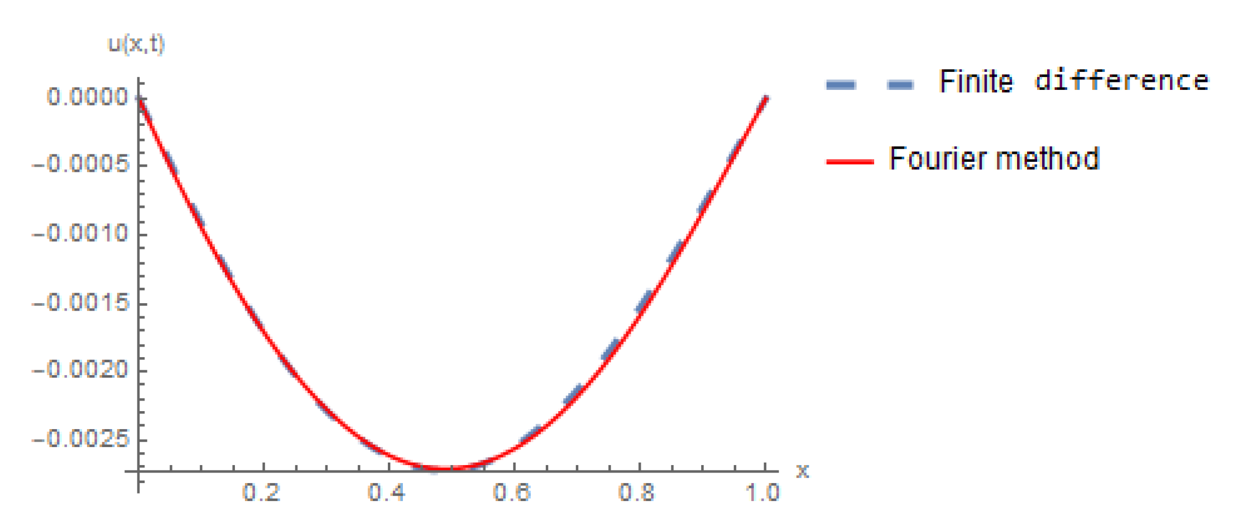
5. Numerical Results

In this section, a numerical example is presented to verify the computational performance and the theoretical results of our proposed schemes.

Example 1.

Consider the following one-dimensional time–space fractional vibration equation.

$$\begin{array}{ccc}\hfill a\frac{{\partial }^{2}u(x,t)}{\partial t^2}& =& \frac{{\partial }^{2}u(x,t)}{\partial x^2}+c_0{D}_{0t}^{\beta }u(x,t)+c_1{D}_{0x}^{\alpha }u(x,t),0<x<L,0<t<T,\hfill \\ \hfill u(0,t)& =& u(L,t)=0,\hfill \\ \hfill u(x,0)& =& 0.1x(1-x),\hfill \\ \hfill u_t(x,0)& =& -x^3,\hfill \end{array}$$

(24)

where $a=1,c_1=0.5,c_0=-1.8,T=1$ and $L=1$ when $0<\alpha ,\beta <2.$ The exact solution of the problem Equation (23) has the following form

$$\begin{array}{c}\hfill U(x,t)=\sum _{m=1}^{\infty }\frac{{\chi }_m\left(x\right)}{\langle {\chi }_m\left(x\right),{\tilde{\chi }}_m\left(x\right)\rangle }\left[Z_m\left(t\right)\langle \psi \left(x\right),{\tilde{\chi }}_m\left(x\right)\rangle +{\tilde{Z}}_m\left(t\right)\langle \phi \left(x\right),{\tilde{\chi }}_m\left(x\right)\rangle \right],\end{array}$$

(25)

hence,

$${\chi }_m\left(x\right)=x+\sum _{n=1}^{\infty }{(-1)}^n\sum _{k=0}^n\frac{\left(\genfrac{}{}{0pt}{}{n}{k}\right)c_1^k{\vartheta }_m^{n-k}}{\Gamma (2n+2-k\alpha )}{x}^{2n+1-k\alpha },$$

(26)

and,

$$Z_m\left(t\right)=t-\frac{{\vartheta }_m{t}^3}{6a}+\sum _{n=1}^{\infty }{(-1)}^{n+1}\sum _{k=0}^n\frac{\left(\genfrac{}{}{0pt}{}{n}{k}\right){(-c_0)}^k{\vartheta }_m^{n+1-k}}{a^{n+1}\Gamma (2n+4-k\beta )}{t}^{2n+3-k\beta },$$

(27)

$${\tilde{Z}}_m\left(t\right)=1-\frac{{\vartheta }_m{t}^2}{2a}+\sum _{n=1}^{\infty }{(-1)}^{n+1}\sum _{k=0}^n\frac{\left(\genfrac{}{}{0pt}{}{n}{k}\right){(-c_0)}^k{\vartheta }_m^{n+1-k}}{a^{n+1}\Gamma (2n+3-k\beta )}{t}^{2n+2-k\beta },$$

(28)

where, the parameter ϑ [19] is an eigenvalues of the Equation (23).

Figure 1 shows the numerical solution of Formula (13) for different $\alpha$ and $\beta$. And, Figure 2 and Figure 3 also show the comparison of the numerical solution with the exact solution when $\alpha =1.5$ and $\beta =1.47$, where we take step size $\tau =h=1/20$.

6. Conclusions

This article has constructed a numerical scheme and an alternating direction implicit scheme for a one-dimensional space-time differential equation with fractional derivatives. The proposed scheme turns out to be unconditionally stable and converges up with the second order accuracy for both variables. Theoretical results are tested using a numerical experiment. In the following works, the comparison of the proposed calculation technology with other existing methods will be continued, and the application of the equation in dynamic systems and optimal control will be considered.

References

1. Podlubny, I. Fractional Differential Equations; Academic Press: New York, NY, USA, 1999. [Google Scholar]
2. Davis, H.T. The Theory of Linear Operators; Myers Press: Bloomington, IN, USA, 2008. [Google Scholar]
3. Sabatier, J.; Agrawal, O.P.; Machado, A.T. Advances in Fractional Calculus. In Heoretical Developments and Applications in Physics and Engineering; Springer: Dordrecht, The Netherlands, 2007. [Google Scholar]
4. Martínez-García, M.; Gordon, T.; Shu, L. Extended Crossover Model for Human-Control of Fractional Order Plants. IEEE Access 2017, 5, 27622–27635. [Google Scholar] [CrossRef]
5. Martínez-García, M.; Zhang, Y.; Gordon, T. Memory Pattern Identification for Feedback Tracking Control in Human-Machine Systems. Hum. Factors 2019. [Google Scholar] [CrossRef] [Green Version]
6. Stamova, I.; Gani, S. Functional and Impulsive Differential Equations of Fractional Order: Qualitative Analysis and Applications; CRC Press: Boca Raton, FL, USA, 2017. [Google Scholar]
7. Luchko, Y. Subordination principles for the multi-dimensional space-time fractional diffusion wave equations. Theor. Probab. Math. Statist. 2019, 98, 127–147. [Google Scholar] [CrossRef] [Green Version]
8. Shallal, M.A.; Jabbar, H.N.; Ali, K.K. Analytical solution for the space-time fractional Klein-Gordon and coupled conformable Boussinesq equations. Results Phys. 2018, 8, 372–378. [Google Scholar] [CrossRef]
9. Luchko, Y.; Goren, R.F. An operationl method for solving fractional differential equations with the caputo derivatives. Acta Math. Vietnam. 1999, 2, 207–233. [Google Scholar]
10. Aleroev, T.S.; Kekharsaeva, E.R. Boundary value problems for differential equations with fractional derivatives. Integr. Transf. Spec. 2017, 12, 900–908. [Google Scholar] [CrossRef]
11. Atangana, A. Fractional Operators With Constant and Variable Order with Application to Geo-Hydrology; Academic Press: Cambridge, MA, USA, 2017. [Google Scholar]
12. Huang, J.F.; Arshad, S.; Jiao, Y.D.; Tang, Y.F. Convolution quadrature methods for time-space fractional nonlinear diffusion wave equations. East Asian J. Appl. Math. 2019, 9, 538–557. [Google Scholar] [CrossRef]
13. Lubich, C. Discretized fractional calculus. SIAM J. Math. Anal. 1986, 17, 704–719. [Google Scholar] [CrossRef]
14. Chen, H.; Lu, S.J.; Chen, W.P. A unified numerical scheme for the multi-term time fractional diffusion and diffusion wave equations with variable coefficients. J. Comput. Appl. Math. 2018, 330, 380–397. [Google Scholar] [CrossRef]
15. Tian, W.Y.; Zhou, H.; Deng, W.H. A class of second order difference approximations for solving space fractional diffusion equations. Math. Comput. 2015, 84, 1703–1727. [Google Scholar] [CrossRef] [Green Version]
16. Sun, Z.Z. The Method of Order Reduction and Its Application to the Numerical Solutions of Partial Differential Equations; Science Press: Beijing, China, 2009. [Google Scholar]
17. Li, C.P.; Zeng, F.Z. Numerical Methods for Fractional Calculu; Chapman and Hall/CRC: New York, NY, USA, 2015. [Google Scholar]
18. Wang, P.D.; Huang, C.M. An energy conservative difference scheme for the nonlinear fractional Schrödinger equations. J. Comput. Phys. 2015, 293, 238–251. [Google Scholar] [CrossRef]
19. Aleroeva, H.; Aleroev, T.S. Some applications of fractional calculus. IOP Conf. Ser. Mater. Sci. Eng. 2020, 747, 012046. [Google Scholar] [CrossRef]
Figure 1. The comparison of the solution (13) at , c 1 = 0.5 , c 0 = 1.8 for different α and β .
Mathematics 08 01069 g001
Figure 2. The exact and numerical solution at c 1 = 0.5 , c 0 = 1.8 when α = 1.5 and β = 1.47 .
Mathematics 08 01069 g002
Figure 3. The comparison of the numerical solution with the exact solution at t = 1 , c 1 = 0.5 and c 0 = 1.8 when α = 1.5 and β = 1.47 .
Mathematics 08 01069 g003