Estimation of Uncertainty in Mortality Projections Using State-Space Lee-Carter Model

Abstract

The study develops alternatives of the classical Lee-Carter stochastic mortality model in assessment of uncertainty of mortality rates forecasts. We use the Lee-Carter model expressed as linear Gaussian state-space model or state-space model with Markovian regime-switching to derive coherent estimates of parameters and to introduce additional flexibility required to capture change in trend and non-Gaussian volatility of mortality improvements. For model-fitting, we use a Bayesian Gibbs sampler. We illustrate the application of the models by deriving the confidence intervals of mortality projections using Lithuanian and Swedish data. The results show that state-space model with Markovian regime-switching adequately captures the effect of pandemic, which is present in the Swedish data. However, it is less suitable to model less sharp but more prolonged fluctuations of mortality trends in Lithuania.

1. Introduction

Mortality projections are used by insurance companies, pension providers and public policy makers for forecasting expected payments of benefits contingent on human lives (such as insurance benefits and pensions) as well as their distribution. Specifically, insurance companies use such projections for pricing of products, solvency calculations and risk assessments. With the upcoming new international insurance accounting standard, the allowance for risk will be required in the financial reporting as well.

Lee-Carter stochastic mortality model is one of the most popular models applied in practice for forecasting expected human mortality and its distribution. Lee and Carter [1] models mortality rates according to the following formula:

$$log\left(m_{x,t}\right)={\alpha }_x+{\kappa }_t{\beta }_x+{\mathcal{E}}_{x,t},$$

(1)

where $m_{x,t}$ is central mortality rate (ratio of the number of deaths to the exposed to risk) for age x in year t, ${\alpha }_x$, ${\kappa }_t$, ${\beta }_x$ are parameters depending on age x or on year t, and ${\mathcal{E}}_{x,t}$ are independent and identically distributed (i.i.d.) random residuals with zero means.

In its original form and according to the later modifications, see Brouhns et al. [2] or Lee and Miller [3] for instance, Lee-Carter model supposes two stage estimation procedure. First, parameters ${\alpha }_x$, ${\kappa }_t$ and ${\beta }_x$ are estimated using the matrix singular value decomposition (SVD) method or by fitting a Poisson bi-linear regression. Secondly, parameter ${\kappa }_t$, which might be interpreted as time varying index representing the general trend of human mortality improvements, is modelled separately as time series, most often as a simple random walk with drift (RWD):

$${\kappa }_t=\mu +{\kappa }_{t-1}+{\nu }_t,$$

(2)

where $\mu$ is the drift (or trend) parameter and ${\nu }_t$ are i.i.d. residuals with zero means.

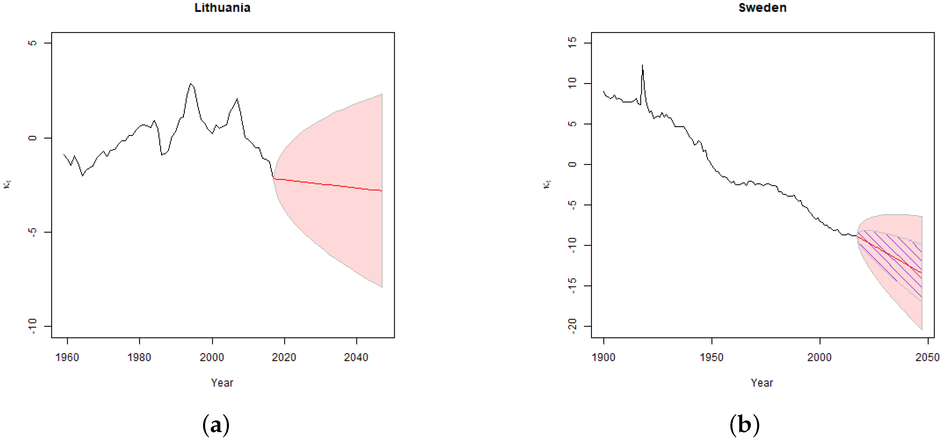
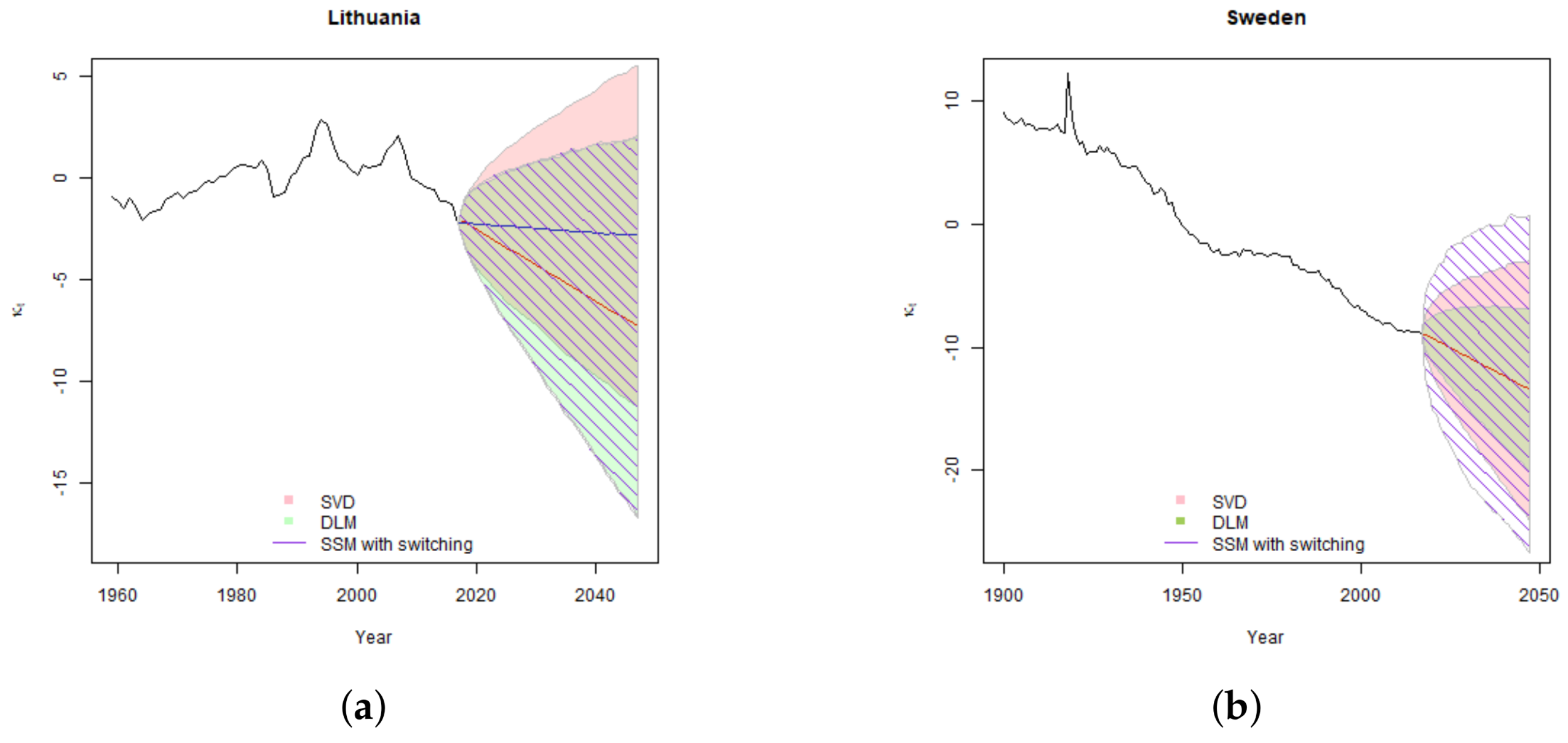
Despite its popularity Lee-Carter model has several limitations. The model ensures adequate fit only if the underlying data contains a stable mortality trend. For example, Figure 1 shows the results of fitting classical Lee-Carter model to mortality data which either has a volatile trend or includes an outlier.

In the Lithuanian case the standard Lee-Carter model produces projections with unacceptably wide confidence intervals due to volatile historic mortality experience which poorly fit a linear trend assumption. The country experienced a sharp increase in mortality rates after the collapse of the Soviet Union (that was experienced by many ex-USSR countries) which was followed by a gradual decline in mortality rates after the country’s independence and the accession to the EU. Consistent Swedish mortality improvement was distorted by the effect of 1918–1920 Spanish flu pandemic. Thus, the estimated variance of the Swedish projections averages the variance observed during the periods of usual mortality development and that of the pandemic period. Figure 1b shows that just one outlier of the year 1918 has a major effect on the estimated confidence intervals of the projected time varying index.

Standard Lee-Carter model has limited possibilities of dealing with such distortions and usually the key practical recipe of achieving adequate fit is to cut the data used for model-fitting to the latest stable mortality period, see Gylys and Šiaulys [4], Lee and Miller [3], Tuljapurkar et al. [5]. In addition, the classical Lee-Carter model projections do not allow for parameter uncertainty. Some authors, e.g., Brouhns et al. [6], Koissi et al. [7], applied bootstrap methods to estimate the effect of uncertainty in estimated parameters. However, the results of such analysis are affected by the general limitations of the Lee-Carter model as described above.

State-space time series models (SSMs) (see Durbin and Koopman [8], Harvey [9], West and Harrison [10]) defined by relations

$${\overline{\mathbf{y}}}_t\sim p\left({\overline{\mathbf{y}}}_t\right|{\overline{\mathbf{x}}}_t),{\overline{\mathbf{x}}}_t\sim p\left({\overline{\mathbf{x}}}_t\right|{\overline{\mathbf{x}}}_{t-1}),$$

where vector ${\overline{\mathbf{y}}}_t$ is observed, vector ${\overline{\mathbf{x}}}_t$ is unobserved state parameter vector, and p is an arbitrary distribution. SSM offers a natural opportunity to extend the Lee-Carter model both in terms of the alternative coherent fitting procedure and the possibility to flex the model by introducing additional parameters to ensure a better fit. A linear Gaussian state-space model, often called Dynamic Linear Model (DLM) is one the most popular SSM in applications This model can be represented by the following two equations:

$${\overline{\mathbf{y}}}_t={\mathbf{Z}}_t{\overline{\mathbf{x}}}_t+{\overline{\epsilon }}_t,{\overline{\mathbf{x}}}_t={\mathbf{U}}_t{\overline{\mathbf{x}}}_{t-1}+{\overline{\eta }}_t,$$

(3)

where ${\overline{\epsilon }}_t\sim N(\overline{0},{\mathbf{H}}_t)$ and ${\overline{\eta }}_t\sim N(\overline{0},{\mathbf{Q}}_t)$ are the Gaussian errors and ${\mathbf{Z}}_t$, ${\mathbf{H}}_t$, ${\mathbf{U}}_t$, ${\mathbf{Q}}_t$ are the parameter matrixes. Thus, we can express Lee-Carter model in state-space representation by treating Equation (1) as observation equation and Equation (2) of the time varying index ${\kappa }_t$ as an the state equation.

State-space models can be traced back to highly influential paper by Kalman [11]. Although initially these methods were applied predominantly in engineering and signal processing, over time it became a recognized statistical modelling technique. Examples of application of the SSMs in mortality analysis are presented by Fung et al. [12], Kogure and Kurachi [13] and Pedroza [14] among others.

As an extension, we applied SSM with regime-switching (SSM with switching). Such models are often referred to multi-process models and are DLMs conditionally on a sequence of indicator variables, which represent varying regimes. In the context of the mortality modelling such regimes may be interpreted as switching between stable and volatile socio-economic development conditions which positively or negatively affect the mortality development. Such models were successfully applied in economics for modelling of business cycles, see for instance Hamilton [15], Kaufmann [16] and Kim and Nelson [17] among others.

Thus, the aim of the paper is to explore the possibilities of SSMs to develop an alternative solution of dealing with the two common general problems, as illustrated above, encountered in practice when modelling mortality. We treat the pandemics, wars, other significant one-off fluctuations in mortality rates as a natural phenomenon to be considered in the projections. We also show how to use flexibility of SSMs to deal with one-time change in socio-economic development, which, for example, was experienced by many Central and Eastern European countries. The focus of the analysis is estimation of confidence intervals of the projected mortality rates, in particular at the tails of the distributions, which is important for insurers’ solvency and economic capital models, rather than just the central mortality forecast. The performance of the models is assessed by using the mortality data of Lithuania and Sweden, but the issues and possible application is not limited to these countries.

We estimate the model parameters using Gibbs sampler, which is the primary Markov chain Monte Carlo (MCMC) method for SSMs with switching. Output from the Gibbs sampler also allows us to take into account parameter uncertainty. For ensuring the comparability of results, we also use the Gibbs sampler for fitting DLMs. For model comparison we use marginal likelihoods estimated with sequential Monte Carlo technique based on auxiliary particle filter.

The study covers ages from 25 to 74 and is primary aimed at the assessment of mortality risk at insurance companies. However, the methods used can be extended to analysis of mortality of older ages and can be used for assessment of longevity risk, which is particular important for pension products providers. For the analysis we use the general population data from Human Mortality Database for ages 25–74 grouped in 5 year age groups for the following periods: Lithuania 1959–2017, Sweden 1900–2017. Human Mortality Database (https://www.mortality.org) is maintained by the University of California, Berkeley (USA), and the Max Planck Institute for Demographic Research (Germany). Data for our research was downloaded in February 2020.

The paper is organized as follows. Section 2 provides an overview of the models used, the Gibbs sampler as well as the methodology used for model comparison. Section 3 provides the detailed description of the algorithms. Section 4 deals with details of the MCMC diagnostics and the model-fitting and comparison results. Section 5 provides overview of the forecasting results. Section 6 concludes the paper with the discussion of the results, implications for the mortality modelling and areas for further research.

2. State-Space Lee-Carter Models

We develop two different specifications of state-space Lee-Carter model: based on DLM and SSM with switching. For comparison we use the results derived by the classical Lee-Carter method fitted using SVD, therefore, some details of the classical model are also provided.

2.1. DLM

By using the general expression (3) of DLM, we can formulate state-space Lee-Carter model by the following two equations:

$$\begin{array}{ccc}\hfill {\overline{\mathbf{y}}}_t& =& (\overline{0},\overline{0},\overline{\beta }){\overline{\mathbf{x}}}_t+{\overline{\epsilon }}_t,{\overline{\epsilon }}_t\sim N(\overline{0},{\mathbf{H}}_t),\hfill \end{array}$$

(4)

$$\begin{array}{ccc}\hfill {\overline{\mathbf{x}}}_t& =& \left(\begin{array}{c}{\mu }_t^{\left(I\right)}\\ {\mu }_t^{\left(II\right)}\\ {\kappa }_t\end{array}\right)=\left(\begin{array}{ccc}1& 0& 0\\ 0& 1& 0\\ 1& {𝟙}_{\{t>T_0\}}& 1\end{array}\right){\overline{\mathbf{x}}}_{t-1}+{\overline{\eta }}_t,{\overline{\eta }}_t\sim N(\overline{0},{\mathbf{Q}}_t).\hfill \end{array}$$

(5)

In the observation Equation (4), symbol ${\overline{\mathbf{y}}}_t$ denotes vector with N coordinates, where N is the total number of age groups. Each coordinate of this vector $x\in \{1,2,\dots ,N\}$ is the specific centered log-mortality rate

$$y_{x,t}=log\left(m_{x,t}\right)-\frac{1}{T}\sum _{t=1}^{T}log\left(m_{x,t}\right).$$

(6)

Parameter $\overline{\beta }$ is a column vector of N age specific parameters ${\beta }_x$, which determine the impact of the time varying index on log-mortality rates. Matrix ${\mathbf{H}}_t$ is a diagonal $N\times N$ matrix with all diagonal elements equal to ${\sigma }_H^2$.

In the state Equation (5), element ${\kappa }_t$ is the time varying index, which represents the general trend of changes in mortality rates with time, ${\mu }_t^{\left(I\right)}$ is the drift of ${\kappa }_t$ which continues for the whole fitting period. Coordinate ${\mu }_t^{\left(II\right)}$ represents the additional drift element in the time period $t>T_0$ and symbol $𝟙$ denote the standard indicator function. Thus, during the periods $t>T_0$ the model assumes that the total drift of parameter ${\kappa }_t$ is ${\mu }_t^{\left(I\right)}+{\mu }_t^{\left(II\right)}$. As in the classical Lee-Carter model, we assume that both drift parameters stay constant during the fitting period and we apply the following covariance matrix of errors of the state parameter ${\overline{\mathbf{x}}}_t$:

$${\mathbf{Q}}_t=\left(\begin{array}{ccc}0& 0& 0\\ 0& 0& 0\\ 0& 0& {\sigma }_Q^2\end{array}\right).$$

The above model maintains many of the features of the classical Lee-Carter model. The time varying index ${\kappa }_t$ follows a RWD. Contrary to the classical Lee-Carter model we allow a one-time change in drift at some time moment $T_0$ but otherwise drifts are not allowed to vary in time. Such structure ensures that the model is sufficiently rigid, which is important for making long-term forecasts. On the other hand, the feature of one-time change in drift allows us to model major changes in environment, which cannot be modelled in the classical model. As in the classical Lee-Carter model the general trend of mortality modelled with parameter ${\kappa }_t$ is translated to age specific log-mortality rates via the parameters ${\beta }_x$, and the random residuals ${\mathcal{E}}_{x,t}$, are assumed to be i.i.d.

In our model, we stochastically assess the deviations from the centered log-mortality rates, and the Lee-Carter parameters ${\alpha }_x$, which represent the general shape of changes in log-mortality rates with age, are expected to be fixed. We set

$${\alpha }_x=\frac{1}{T}\sum _{t=1}^{T}log\left(m_{x,t}\right)$$

for $x=1,\dots ,N$, as in the most of the classical Lee-Carter model’s applications, and deduct it from log-mortality rates before starting the fitting process, see Equation (6). Overall, in applications of the Lee-Carter model, parameter ${\alpha }_x$ has proved to be one of the most predictable model parameters. For example, in the bootstrap analysis performed by Koissi [7], variation in the estimates of parameter ${\alpha }_x$ was predominantly related to very young ages (below 20 years) and old ages above 80 years, and for the remaining ages was very stable. Therefore, we consider that the simplification of fixing ${\alpha }_x$ parameter does not have a significant effect on the results of the analysis.

As in the classical Lee-Carter model we apply the following identifiability constraint for parameters ${\beta }_x$:

$$\sum _{x=1}^N{\beta }_x=1.$$

The constraint is applied in step $\left(\mathrm{vi}\right)$ of algorithm $\mathcal{A}2$ presented in Section 3.2, where the estimated parameters ${\beta }_x$ are re-weighted with the corresponding adjustments made to the mean and scale of the estimates of ${\kappa }_t$. Thus, after the re-weighting the distribution of the term $(\overline{0},\overline{0},\overline{\beta }){\overline{\mathbf{x}}}_t$ is unchanged.

The key feature of the SSMs is that they enable estimation of the distribution of each of the unobservable parameters ${\overline{\mathbf{x}}}_t$, by using the observed data ${\overline{\mathbf{y}}}_1,\dots ,{\overline{\mathbf{y}}}_t$. The recursive algorithm, called Kalman filter, which is based on the method of orthogonal projections and uses the features of the conditional Normal distribution, updates the estimate of the mean and variance of ${\overline{\mathbf{x}}}_{t-1}$ with the new evidence contained in ${\overline{\mathbf{y}}}_t$ in order to derive the mean and variance of ${\overline{\mathbf{x}}}_t$. For the equation of the basic Kalman filter, see step $\left(\mathrm{i}\right)$ of algorithm $\mathcal{A}1$ described in Section 3.1. Thus, assuming that the collection of the model parameters $\psi =\{\overline{\beta },{\sigma }_Q^2,{\sigma }_H^2,\overline{\mu }\}$, $\overline{\mu }={\left({\mu }^{\left(I\right)},{\mu }^{\left(II\right)}\right)}^{⊺}$, is known, we can run the filter for all $t\in \{1,\dots ,T\}$ and derive the distribution of $\{{\overline{\mathbf{x}}}_1,\dots ,{\overline{\mathbf{x}}}_T\}$, which shall contain the mean and variance of time varying index ${\kappa }_t$ for $t\in \{1,\dots ,T\}$. The detailed description of the method used to estimate the parameter collection $\psi$ is presented in Section 2.3.

2.2. SSM with Switching

The basic equations of our state-space Lee-Carter model with switching remain (4) and (5). The key difference from the previous model is that we assume that the error terms ${\overline{\eta }}_t$, $t\in \{1,\dots ,T\}$, follow a mixture of two zero mean Normal distributions with the following covariance matrixes:

$${\mathbf{Q}}_t^{\left(0\right)}=\left(\begin{array}{ccc}0& 0& 0\\ 0& 0& 0\\ 0& 0& {\left({\sigma }_Q^{\left(0\right)}\right)}^2\end{array}\right),{\mathbf{Q}}_t^{\left(1\right)}=\left(\begin{array}{ccc}0& 0& 0\\ 0& 0& 0\\ 0& 0& {\left({\sigma }_Q^{\left(1\right)}\right)}^2\end{array}\right),$$

each of them corresponding to one of the two regimes. We restrict ${\left({\sigma }_Q^{\left(0\right)}\right)}^2⩽{\left({\sigma }_Q^{\left(1\right)}\right)}^2$ and use a binary index $s_t$: low variance regime $s_t=0$ and high variance regime $s_t=1$. Therefore, in SSM with switching the errors of the parameter ${\kappa }_t$

$$\sum _{i=0}^1\mathbb{P}(s_t=i)N\left(0,{\left({\sigma }_Q^{\left(i\right)}\right)}^2\right),$$

depending on its parametrization may have much heavier tails with respect to tail of standard Normal distribution.

The switching between the two regimes is assumed to follow the Markov process with constant transition probabilities as introduced by Hamilton [15]. We define two probabilities

$${\pi }^{\left(0\right)}=\mathbb{P}\left(s_t=0|s_{t-1}=0\right),{\pi }^{\left(1\right)}=\mathbb{P}\left(s_t=1|s_{t-1}=1\right),$$

which imply that:

$$\mathbb{P}\left(s_t=1|s_{t-1}=0\right)=1-{\pi }^{\left(0\right)},\mathbb{P}\left(s_t=0|s_{t-1}=1\right)=1-{\pi }^{\left(1\right)}.$$

Consequently, the parameter collection of the model with switching ${\psi }^{\left(s\right)}=\{\overline{\beta },{\overline{\sigma }}_Q,{\sigma }_H^2,\overline{\mu },\overline{\pi }\}$ contains three extra parameters: vector of variances ${\overline{\sigma }}_Q={\left({\left({\sigma }_Q^{\left(0\right)}\right)}^2,{\left({\sigma }_Q^{\left(1\right)}\right)}^2\right)}^{⊺}$ instead of one variance ${\sigma }_Q^2$ and vector of transition probabilities $\overline{\pi }={\left({\pi }^{\left(0\right)},{\pi }^{\left(1\right)}\right)}^{⊺}$.

Conditionally on values of ${\kappa }_t$, $t\in \{1,\dots ,T\}$, we can recursively estimate probabilities of $s_t=0$ and $s_t=1$, by taking into account the corresponding probabilities at the time moment $t-1$, as well as the likelihood of being in a particular state, which is driven by the deviation of the change ${\kappa }_t-{\kappa }_{t-1}$ from its expected value ${\mu }_t^{\left(I\right)}+{𝟙}_{\{t>T_0\}}{\mu }_t^{\left(II\right)}$: the higher the deviation is, the more likely is that the process has moved to high variance regime. For details see step $\left(\mathrm{ii}\right)$ of algorithm $\mathcal{A}3$ described in Section 3.3.

Conditionally on values of $s_t$, $t\in \{1,\dots ,T\}$, we can apply the basic Kalman filter as described in Section 2.1. The only difference is that the matrix ${\mathbf{Q}}_t$ can vary in different update steps of the filter; however, this does not change the basic operation of the algorithm.

The key benefit from using the SSM with switching is that it enables us to segregate the total variance of ${\kappa }_t$, which is generally recognized to be the key source of variability of mortality rates, into the variance during the periods of the “normal” socio-economic development and the variance during the periods such as epidemics, wars, changes economic and political systems, etc. As shown in Figure 1, the development of the general mortality trend may be far from constant, therefore, the classical Lee-Carter approach, which averages the variance of ${\kappa }_t$ over the fitting periods might miss important features of the real life development, especially when the purpose of the analysis is estimation of the confidence intervals of the mortality forecasts rather than just the central forecast.

2.3. Parameter Estimation with Gibbs Sampler

There are two main approaches to fitting of SSMs: maximum likelihood (MLE) and Bayesian Markov Chain Monte Carlo (MCMC). For estimation of the parameter collection $\psi$ of DLM Lee-Carter we can easily apply MLE, see e.g., [12]. However, as noted by Frühwirth–Schnatter [18], in case of SSM with switching the marginal likelihood where both latent processes $\overline{\mathbf{x}}$ and s are integrated out, is not available in the closed form. In addition, MLE does not explicitly allow for uncertainty in model parameters, which is an important element in satisfying our aim to estimate realistic confidence intervals of the forecasts.

Therefore, for model-fitting we apply MCMC method called Gibbs sampler, which was also used in some earlier applications of the state-space Lee-Carter model without regime-switching by Fung et al. [12], Kogure and Kurachi [13], Pedroza [14]. The Gibbs sampler draws samples of parameter values from sequentially updated conditional distributions. Thus, if we have a parameter vector $\overline{\mathsf{\Lambda }}=({\mathsf{\Lambda }}_1,{\mathsf{\Lambda }}_2,\dots ,{\mathsf{\Lambda }}_M)$, the Gibbs sampler at each iteration $j=1,2,\dots$ would sequentially draw samples of ${\mathsf{\Lambda }}_i^j$ for $i\in \{1,2,\dots ,M\}$ from $\{{\mathsf{\Lambda }}_1^j,\dots ,{\mathsf{\Lambda }}_{i-1}^j,{\mathsf{\Lambda }}_{i+1}^{j-1},\dots ,{\mathsf{\Lambda }}_M^{j-1}\}$, where ${\mathsf{\Lambda }}_i^j$ denotes draw of parameter ${\mathsf{\Lambda }}_i$ at j iteration. As shown by Geman and Geman [19] under certain mild conditions the distribution of draws ${\overline{\mathsf{\Lambda }}}^j$ converge to the true distribution of $\overline{\mathsf{\Lambda }}$ if $j\to \infty$, independently of the starting values of ${\overline{\mathsf{\Lambda }}}^1=({\mathsf{\Lambda }}_1^1,{\mathsf{\Lambda }}_2^1,\dots ,{\mathsf{\Lambda }}_M^1)$.

The general difficulty in constructing and using the Gibbs sampler is the requirement at each step to have conditional distributions of the sampled parameters. In our case, conditional distributions of time invariant parameters can be derived from Equations (4) and (5); however, the complication arises of implementing a proper conditional sampler of the unobserved state parameter ${\overline{\mathbf{x}}}_t$ and, in the case of model with switching, the collection vector of regimes $\overline{s}$. This issue was successfully resolved by Forward Filtering Backwards Sampling (FFBS) algorithm presented in algorithm $\mathcal{A}1$ in Section 3.1, see also Carter and Kohn [20] and Frühwirth-Schnatter [21] for additional information.

We note that the Gibbs sampler is a Bayesian estimation method, thus in addition to the estimated parameters the conditional distributions at each step of the sampling scheme depend on the selected priors. We denote the collection of priors for DLM and SSM with switching $\Theta =\{{\overline{m}}_0,{\mathbf{M}}_0,g_0,G_0,b_0,B_0\}$ and ${\Theta }^{\left(s\right)}=\{{\overline{m}}_0,{\mathbf{M}}_0,g_0,G_0,b_0,B_0,p_0^{\left(1\right)},p_0^{\left(2\right)}\}$ respectively, where $\{{\overline{m}}_0,{\mathbf{M}}_0\}$ and $\{b_0,B_0\}$ are conjugate multivariate/univariate Normal priors, $\{g_0,G_0\}$ are conjugate gamma priors, and $\left\{p_0^{\left(1\right)},p_0^{\left(2\right)}\right\}$ are conjugate beta priors.

The details of descriptions of the parameter estimation algorithms are provided in Section 3.2 and Section 3.3.

2.4. Forecasting

As noted in the previous section, Gibbs sampler after its convergence produces draws from the posterior joint distribution of parameters. Thus, after discharging certain number of initial draws (called burn or warm-up phase) we can use the draws as an input for the forecasting simulations of the state-space models. For both models DLM and SSM with switching we simulate the projected mortality rates for periods $T+1,\dots ,T+K$ in the following way.

(i) 

Depending on the model, DLM or SSM with switching, sample parameter collection ψ or ${\psi }^{\left(s\right)}$ from the matrix of Gibbs sampler draws obtained during the model-fitting phase after the warm-up. In this step, we are sampling the parameter values from their joint posterior distributions.

(ii) 

For SSM with switching, draw sample of regime indicators $\overline{\mathbf{s}}$ for the forecasted period using step $\left(\mathrm{ii}\right)$ of the algorithm $\mathcal{A}3$ (see Section 3.3). As ${\kappa }_t$ are not available for time moments $t=T+1,\dots ,T+K$, multiplication by the probability $\mathbb{P}\left({\overline{\mathbf{x}}}_t\right|s_t)$ in position (ii.2) of algorithm $\mathcal{A}3$ may be disregarded.

(iii) 

For SSM with switching, using sampled parameters $\overline{\mu }$ and ${\overline{\sigma }}_Q$ and regime vector $\overline{s}$ from step $\left(\mathrm{ii}\right)$ simulate ${\kappa }_t$ for time moments $t=T+1,\dots ,T+K$ by supposing that

$${\kappa }_t\sim N\left({\kappa }_{t-1}+{\mu }^{\left(I\right)}+{\mu }^{\left(II\right)},{\left({\sigma }_Q^{\left(i\right)}\right)}^2\right)$$

where ${\left({\sigma }_Q^{\left(i\right)}\right)}^2$ is switching between ${\left({\sigma }_Q^{\left(0\right)}\right)}^2$ and ${\left({\sigma }_Q^{\left(1\right)}\right)}^2$ depending on the simulated $\overline{s}$.

In case of DLM, use ${\sigma }_Q^2$ as a fixed variance.

(iv) 

Using sampled parameters $\overline{\beta }$ and ${\sigma }_H^2$ and sampled vector $\overline{\kappa }$ from step (iii), as well as allowing that errors are i.i.d., simulate $y_{x,t}$ for time moments $t=T+1,\dots ,T+K$ and age groups $x=1,\dots ,N$ by supposing that $y_{x,t}\sim N\left({\beta }_x{\kappa }_t,{\sigma }_H^2\right).$

(v) 

Calculate mortality rates, having in mind that $m_{x,t}=exp\{y_{x,t}+{\alpha }_x\}$ for all possible x and t.

In case of the classical Lee-Carter model, we do not have draws from the posterior distribution of the parameters. We can partially allow for parameter uncertainty in the classical Lee-Carter model by allowing for uncertainty of the drift, see [3], the distribution of which follows from the RWD assumption of ${\kappa }_t$. Except for ${\mu }^{\left(I\right)}$, for the simulation we use fixed parameters, estimated via SVD and time series fitting process. Therefore, the classical Lee-Carter model provides less comprehensive treatment of parameter uncertainty than SSMs. For the classical Lee-Carter model we simulate the projected mortality rates for time moments $t=T+1,\dots ,T+K$ by the following algorithm.

(i) 

Draw ${\mu }_{sim}^{\left(I\right)}$ from ${\mu }_{sim}^{\left(I\right)}\sim N\left({\mu }^{\left(I\right)},{\sigma }_Q^2/T\right)$.

(ii) 

Simulate ${\kappa }_t$ for $t=T+1,\dots ,T+K$ from ${\kappa }_t\sim N\left({\kappa }_{t-1}+{\mu }_{sim}^{\left(I\right)},{\sigma }_Q^2\right)$.

(iii) 

Simulate $y_{x,t}$ for $t=T+1,\dots ,T+K$ by supposing that $y_{x,t}\sim N\left({\beta }_x{\kappa }_t,{\sigma }_H^2\right)$.

(iv) 

Calculate mortality rates for all possible x and t, by formula $m_{x,t}=exp\{y_{x,t}+{\alpha }_x\}.$

2.5. Comparison of State-Space Models

For the state-space model comparison, we use marginal likelihood. We apply the following formula by Chib [22]:

$$m\left({\mathbf{Y}}_{1:T}\right)=m\left({\mathbf{Y}}_{1:T}|\widehat{\psi }\right)+m\left(\widehat{\psi }\right)-m\left(\widehat{\psi }|{\mathbf{Y}}_{1:T}\right),$$

where ${\mathbf{Y}}_{1:T}=\left({\overline{\mathbf{y}}}_1,{\overline{\mathbf{y}}}_2,\dots ,{\overline{\mathbf{y}}}_T\right)$, $m\left({\mathbf{Y}}_{1:T}\right)$ is the marginal log-likelihood, $m\left({\mathbf{Y}}_{1:T}|\widehat{\psi }\right)$ is the log-likelihood conditional on the estimated parameters, $m\left(\widehat{\psi }\right)$ is log density of prior at $\widehat{\psi }$ and $m\left(\widehat{\psi }|{\mathbf{Y}}_{1:T}\right)$ is the log density of posterior at $\widehat{\psi }$.

Term $m\left({\mathbf{Y}}_{1:T}|\widehat{\psi }\right)$ can be calculated in the closed form for DLM, but for SSM with switching the likelihood function would be a mixture of $2^T$ Normal distributions, the direct assessment of which is not practical. Therefore, we use the sequential Monte Carlo method based on auxiliary particle filter of Pitt and Shephard [23] which was adapted to SSM with switching by Kaufmann [16]. The details of the algorithm are provided in Section 3.4.

The term $m\left(\widehat{\psi }|{\mathbf{Y}}_{1:T}\right)$ we estimate similarly as in [22] by using the sequentially running Gibbs sampler for each of the parameters in the collection $\psi =\{{\psi }_1,\dots ,{\psi }_L\}$ and estimating their posterior likelihood at the mean points of $\widehat{\psi }$ from MCMC runs by the following algorithm:

• Estimate $m\left({\psi }_1\right|{\mathbf{Y}}_{1:T})$ as a mean of the appropriate likelihood function of the parameter ${\psi }_1$ evaluated over the parameters of MCMC runs of the Gibbs sampler sampled as described in Section 3.2 and Section 3.3.
• Estimate $m\left({\psi }_2\right|{\mathbf{Y}}_{1:T},{\widehat{\psi }}_1)$ by fixing the parameter ${\psi }_1$ at the value ${\widehat{\psi }}_1$ and by performing additional run of Gibbs sampler as in the first step.
• - - -
• Estimate $m\left({\psi }_L\right|{\mathbf{Y}}_{1:T},{\widehat{\psi }}_1,{\widehat{\psi }}_2,\dots ,{\widehat{\psi }}_{L-1})$ by fixing the parameters ${\psi }_1,{\psi }_2,\dots ,{\psi }_{L-1}$ at the values ${\widehat{\psi }}_1,{\widehat{\psi }}_2,\cdots ,{\widehat{\psi }}_{L-1}$ and by performing additional run of Gibbs sampler as in the first step.

At the end we calculate the total posterior log-likelihood:

$$m\left(\widehat{\psi }\right|{\mathbf{Y}}_{1:T})=m\left({\psi }_1\right|{\mathbf{Y}}_{1:T})+m\left({\psi }_2\right|{\mathbf{Y}}_{1:T},{\widehat{\psi }}_1)+\dots +m\left({\psi }_L\right|{\mathbf{Y}}_{1:T},{\widehat{\psi }}_1,{\widehat{\psi }}_2,\dots ,{\widehat{\psi }}_{L-1}).$$

3. Algorithms

3.1. Forward Filtering Backwards Sampling (FFBS) Algorithm $\mathcal{A}$1

(i) Conditionally on the initial distribution ${\overline{\mathbf{x}}}_1\sim N({\overline{a}}_1,{\mathbf{P}}_1)$, which we assume to be known, for $t\in \{1,2,\dots ,T\}$ run the Kalman filter recursion in order to obtain estimated distributions ${\overline{\mathbf{x}}}_{t|t}\sim N({\overline{a}}_{t|t},{\mathbf{P}}_{t|t})$ of unobserved state parameter vector given the observation ${\overline{\mathbf{y}}}_t$, as well as the distribution of the one step ahead predictions ${\overline{\mathbf{x}}}_{t+1}\sim N({\overline{a}}_{t+1},{\mathbf{P}}_{t+1})$. Using the general Kalman filter equations, see for instance, Chapter 4 by Durbin and Koopman [8], we derive the following recursion formulas for the state-space Lee-Carter model mentioned in Equations (4) and (5):

$$\begin{array}{cc}{\overline{a}}_{t|t}={\overline{a}}_t+{\mathbf{P}}_t\left(\begin{array}{c}{\overline{0}}^{⊺}\\ {\overline{0}}^{⊺}\\ {\overline{\beta }}^{⊺}\end{array}\right){\mathbf{F}}_t^{-1}{\overline{\nu }}_t,& {\mathbf{P}}_{t|t}={\mathbf{P}}_t-{\mathbf{P}}_t\left(\begin{array}{c}{\overline{0}}^{⊺}\\ {\overline{0}}^{⊺}\\ {\overline{\beta }}^{⊺}\end{array}\right){\mathbf{F}}_t^{-1}(\overline{0},\overline{0},\overline{\beta }){\mathbf{P}}_t,\hfill \\ {\overline{a}}_{t+1}={\overline{a}}_t+{\mathbf{K}}_t{\overline{\nu }}_t,& {\mathbf{P}}_{t+1}={\mathbf{P}}_t{(\mathbf{I}-{\mathbf{K}}_t(\overline{0},\overline{0},\overline{\beta }))}^{⊺}+{\mathbf{Q}}_t,\hfill \\ {\overline{\nu }}_t={\overline{\mathbf{y}}}_t-(\overline{0},\overline{0},\overline{\beta }){\overline{a}}_t,& {\mathbf{F}}_t=(\overline{0},\overline{0},\overline{\beta }){\mathbf{P}}_t\left(\begin{array}{c}{\overline{0}}^{⊺}\\ {\overline{0}}^{⊺}\\ {\overline{\beta }}^{⊺}\end{array}\right)+{\mathbf{H}}_t,\hfill \\ {\mathbf{K}}_t={\mathbf{P}}_t\left(\begin{array}{c}{\overline{0}}^{⊺}\\ {\overline{0}}^{⊺}\\ {\overline{\beta }}^{⊺}\end{array}\right){\mathbf{F}}_t^{-1},\end{array}$$

where $t\in \{1,2,\dots ,T\}$, ${\mathbf{F}}_t$ is estimated covariance matrix of the observation, ${\nu }_t$ is an estimated residual, $\mathbf{I}$ is an identity matrix, and the matrix ${\mathbf{K}}_t$ is called the Kalman gain.

(ii)  Sample ${\widetilde{\overline{\mathbf{x}}}}_T$ by supposing that ${\overline{\mathbf{x}}}_T\sim N({\overline{a}}_{T|T},{\mathbf{P}}_{T|T})$.

(iii)  Treat one step forward sample as an observation and apply the Kalman filter to it.

According to Carter and Kohn [20], for $t=T-1,T-2,\dots ,1$, we should sample ${\widetilde{\overline{\mathbf{x}}}}_t$ by supposing that ${\overline{\mathbf{x}}}_t\sim N({\overline{a}}_{t|t,{\widetilde{\overline{\mathbf{x}}}}_{t+1}},{\mathbf{P}}_{t|t,{\widetilde{\overline{\mathbf{x}}}}_{t+1}})$, with

$$\begin{array}{ccc}\hfill {\overline{a}}_{t|t,{\widetilde{\overline{\mathbf{x}}}}_{t+1}}& =& {\overline{a}}_{t|t}+{\mathbf{P}}_{t|t}{\mathbf{P}}_{t+1}^{-1}\left({\widetilde{\overline{\mathbf{x}}}}_{t+1}-{\overline{a}}_{t+1}\right),\hfill \\ \hfill {\mathbf{P}}_{t|t,{\widetilde{\overline{\mathbf{x}}}}_{t+1}}& =& {\mathbf{P}}_{t|t}-{\mathbf{P}}_{t|t}{\mathbf{P}}_{t+1}^{-1}{\mathbf{P}}_{t|t}.\hfill \end{array}$$

3.2. Gibbs Sampler Algorithm $\mathcal{A}$2 for DLM

(o)  Initiate the sampler using an arbitrary starting parameter collection $\psi =\{\overline{\beta },{\sigma }_Q^2,{\sigma }_H^2,\overline{\mu }\}$ and collection of priors $\Theta =\{{\overline{m}}_0,{\mathbf{M}}_0,g_0,G_0,b_0,B_0\}$.

(i)  Sample

$${\widetilde{\overline{\mathbf{x}}}}_t={\left({\mu }_t^{\left(I\right)},{\mu }_t^{\left(II\right)},{\kappa }_t\right)}^{⊺},$$

conditionally on ψ, and store vector $\overline{\kappa }$ of values ${\kappa }_t$ by applying FFBS algorithm $\mathcal{A}1$ with the initial distribution

$${\overline{\mathbf{x}}}_1\sim N\left({\left({\mu }^{\left(I\right)},{\mu }^{\left(II\right)},{\kappa }_0\right)}^{⊺},\left(\begin{array}{ccc}0& 0& 0\\ 0& 0& 0\\ 0& 0& {\sigma }_0^2\end{array}\right)\right)$$

Simulation results are usually insensitive to selection of ${\kappa }_0$, provided ${\sigma }_0^2$ be sufficiently large. We use ${\sigma }_0^2=10$.

(ii)  Sample $\overline{\mu }={({\mu }^{\left(I\right)},{\mu }^{\left(II\right)})}^{⊺}$ conditionally on $\overline{\kappa }$ and ${\sigma }_Q^2$, from the bivariate Normal distribution

$$N\left({\left({\mathbf{M}}_0^{-1}+\frac{1}{{\sigma }_Q^2}{\mathbf{X}}^{⊺}\mathbf{X}\right)}^{-1}\left({\mathbf{M}}_0^{-1}{\overline{m}}_0+\frac{1}{{\sigma }_Q^2}{\mathbf{X}}^{⊺}\Delta \overline{\kappa }\right),{\left({\mathbf{M}}_0^{-1}+\frac{1}{{\sigma }_Q^2}{\mathbf{X}}^{⊺}\mathbf{X}\right)}^{-1}\right),$$

where $\Delta \overline{\kappa }$ is a vector of changes in ${\kappa }_t$, while $\mathbf{X}$ is a matrix of dimension $T\times 2$ with the form

$$\mathbf{X}=\left(\begin{array}{cc}1& 0\\ ⋮& ⋮\\ 1& 0\\ 1& 1\\ ⋮& ⋮\\ 1& 1\end{array}\right),$$

where number of the first lines $T_0⩽T$ is the number of periods before change in trend of ${\kappa }_t$ occurred.

(iii)  Sample ${\sigma }_Q^2$, conditionally on $\overline{\kappa }$ and $\overline{\mu }$, from the inverse Gamma distribution

$$IG\left(G_0+\frac{T}{2},g_0+\frac{1}{2}\sum _{t=1}^T{\left({\kappa }_t-{\kappa }_{t-1}-{\mu }^{\left(I\right)}-{𝟙}_{\{t>T_0\}}{\mu }^{\left(II\right)}\right)}^2\right),$$

where ${𝟙}_{\{t>T_0\}}$ is the standard indicator function.

(iv)  Sample $\overline{\beta }$, conditionally on $\overline{\kappa }$ and ${\sigma }_H^2$, from the Normal distribution.

Considering that we assume that the matrix of measurement errors ${\mathbf{H}}_t$ is diagonal, we can sample ${\beta }_x$ for each age group $x\in \{1,2,\dots ,N\}$ separately:

$${\beta }_x\sim N\left({\left(B_0^{-1}+\frac{1}{{\sigma }_H^2}{\overline{\kappa }}^{⊺}\overline{\kappa }\right)}^{-1}\left(B_0^{-1}{b}_0+\frac{1}{{\sigma }_H^2}{\overline{\kappa }}^{⊺}{\overline{\mathbf{y}}}_x\right),{\left(B_0^{-1}+\frac{1}{{\sigma }_H^2}{\overline{\kappa }}^{⊺}\overline{\kappa }\right)}^{-1}\right),$$

where ${\overline{\mathbf{y}}}_x$ is a vector of centered observations for age group x.

(v)  Sample ${\sigma }_H^2$, conditionally on $\overline{\kappa }$ and $\overline{\beta }$, from the inverse Gamma distribution:

$$IG\left(G_0+\frac{TN}{2},g_0+\frac{1}{2}\sum _{x=1}^N\sum _{t=1}^T{(y_{x,t}-{\beta }_x{\kappa }_t)}^2\right).$$

(vi) Reweight $\overline{\beta }$ and related parameters to ensure that the sum of elements of $\overline{\beta }$ is equal to unit. We proceed as follows:

$$\begin{array}{c}\hfill {\overline{\beta }}^{rew}=\overline{\beta }/\sum _{x=1}^N{\beta }_x,{\overline{\mu }}^{rew}=\overline{\mu }\sum _{x=1}^N{\beta }_x,{\left({\sigma }_Q^2\right)}^{rew}={\sigma }_Q^2{\left(\sum _{x=1}^N{\beta }_x\right)}^2.\end{array}$$

(vii) Collect the updated parameters to collection ψ and proceed to step (i).

3.3. Gibbs Sampler Algorithm $\mathcal{A}$3 for SSM with Switching

(o)  Initiate the sampler using an arbitrary starting parameter collection ${\psi }^{\left(s\right)}=\{\overline{\beta },{\overline{\sigma }}_Q,{\sigma }_H^2,\overline{\mu },\overline{\pi }\}$, collection of priors ${\Theta }^{\left(s\right)}=\{{\overline{m}}_0,{\mathbf{M}}_0,g_0,G_0,b_0,B_0,p_0^{\left(1\right)},p_0^{\left(2\right)}\}$ and an arbitrary vector $\overline{s}=(s_0,s_1,\dots ,s_T)$.

(i)  Sample

$${\widetilde{\overline{\mathbf{x}}}}_t={\left({\mu }_t^{\left(I\right)},{\mu }_t^{\left(II\right)},{\kappa }_t\right)}^{⊺},$$

conditionally on ${\psi }^{\left(s\right)}$ and the regime vector $\overline{\mathbf{s}}$, and store vector $\overline{\kappa }$ of values ${\kappa }_t$ by applying FFBS algorithm $\mathcal{A}1$ with the initial distribution

$${\overline{\mathbf{x}}}_1\sim N\left({\left({\mu }^{\left(I\right)},{\mu }^{\left(II\right)},{\kappa }_0\right)}^{⊺},\left(\begin{array}{ccc}0& 0& 0\\ 0& 0& 0\\ 0& 0& {\sigma }_0^2\end{array}\right)\right)$$

Simulation results are usually insensitive to selection of ${\kappa }_0$, provided ${\sigma }_0^2$ be sufficiently large. We use ${\sigma }_0^2=10$.

(ii)  Sample vector $\overline{s}$, conditionally on $\overline{\kappa }$, ${\overline{\sigma }}_Q$, $\overline{\mu }$ and $\overline{\pi }$ in the following way:

(ii.1) Calculate the initial probabilities of the two regimes by assuming that the filter is initialized with the following stationary Markov chain probabilities:

$$\mathbb{P}(s_0=0)=\frac{1-{\pi }^{\left(1\right)}}{2-{\pi }^{\left(0\right)}-{\pi }^{\left(1\right)}},\mathbb{P}(s_0=1)=\frac{1-{\pi }^{\left(0\right)}}{2-{\pi }^{\left(0\right)}-{\pi }^{\left(1\right)}}.$$

(ii.2)  For $t\in \{1,2,\dots ,T\}$ use the recursive procedure described in [20]:

• Calculate the priors

  $$\begin{array}{ccc}\hfill \mathbb{P}(s_t=0|{\overline{\mathbf{x}}}_{t-1})& =& \mathbb{P}\left(s_{t-1}=0|{\overline{\mathbf{x}}}_{t-1}\right){\pi }^{\left(0\right)}+\mathbb{P}\left(s_{t-1}=1|{\overline{\mathbf{x}}}_{t-1}\right)(1-{\pi }^{\left(1\right)}),\hfill \\ \hfill \mathbb{P}(s_t=1|{\overline{\mathbf{x}}}_{t-1})& =& \mathbb{P}\left(s_{t-1}=1|{\overline{\mathbf{x}}}_{t-1}\right){\pi }^{\left(1\right)}+\mathbb{P}\left(s_{t-1}=0|{\overline{\mathbf{x}}}_{t-1}\right)(1-{\pi }^{\left(0\right)}).\hfill \end{array}$$
• Calculate the posteriors

  $$\begin{array}{ccc}\hfill {\mathbb{P}}^{*}(s_t=0|{\overline{\mathbf{x}}}_t)& =& \mathbb{P}(s_t=0|{\overline{\mathbf{x}}}_{t-1})\mathbb{P}({\overline{\mathbf{x}}}_t={\overline{\mathbf{X}}}_t|s_t=0),\hfill \\ \hfill {\mathbb{P}}^{*}(s_t=1|{\overline{\mathbf{x}}}_t)& =& \mathbb{P}(s_t=1|{\overline{\mathbf{x}}}_{t-1})\mathbb{P}({\overline{\mathbf{x}}}_t={\overline{\mathbf{X}}}_t|s_t=1);\hfill \end{array}$$
  In our case for $i\in \{0,1\}$ probability $\mathbb{P}({\overline{\mathbf{x}}}_t={\overline{\mathbf{X}}}_t|s_t=i)$ should be calculated by Normal distribution with mean ${\kappa }_t-{\kappa }_{t-1}-{\mu }^{\left(I\right)}-{\mu }^{\left(II\right)}{𝟙}_{\{t>T_0\}}$ and variance ${\left({\sigma }_Q^{\left(i\right)}\right)}^2$.
• Standardize the posteriors

  $$\begin{array}{ccc}\hfill \mathbb{P}(s_t=0|{\overline{\mathbf{x}}}_t)& =& \frac{{\mathbb{P}}^{*}(s_t=0|{\overline{\mathbf{x}}}_t)}{{\mathbb{P}}^{*}(s_t=0|{\overline{\mathbf{x}}}_t)+{\mathbb{P}}^{*}(s_t=1|{\overline{\mathbf{x}}}_t)},\hfill \\ \hfill \mathbb{P}(s_t=1|{\overline{\mathbf{x}}}_t)& =& \frac{{\mathbb{P}}^{*}(s_t=1|{\overline{\mathbf{x}}}_t)}{{\mathbb{P}}^{*}(s_t=0|{\overline{\mathbf{x}}}_t)+{\mathbb{P}}^{*}(s_t=1|{\overline{\mathbf{x}}}_t)}.\hfill \end{array}$$

(ii.3)  Sample $s_T$ from the Bernoulli distribution with the success probability $\mathbb{P}(s_T=1|{\overline{\mathbf{x}}}_T)$.

(ii.4)  For $t=T-1,T-2,\dots ,1$ sample $s_t$ recursively from the Bernoulli distribution with the one of the following success probabilities depending on the value of $s_{t+1}$:

$$\begin{array}{ccc}\hfill \mathbb{P}(s_t=1|{\overline{\mathbf{x}}}_t,s_{t+1}=0)& =& \frac{(1-{\pi }^{\left(1\right)})\mathbb{P}(s_t=1|{\overline{\mathbf{x}}}_t)}{(1-{\pi }^{\left(1\right)})\mathbb{P}(s_t=1|{\overline{\mathbf{x}}}_t)+{\pi }^{\left(0\right)}\mathbb{P}(s_t=0|{\overline{\mathbf{x}}}_t)},\hfill \\ \hfill \mathbb{P}(s_t=1|{\overline{\mathbf{x}}}_t,s_{t+1}=1)& =& \frac{{\pi }^{\left(1\right)}\mathbb{P}(s_t=1|{\overline{\mathbf{x}}}_t)}{{\pi }^{\left(1\right)}\mathbb{P}(s_t=1|{\overline{\mathbf{x}}}_t)+(1-{\pi }^{\left(0\right)})\mathbb{P}(s_t=0|{\overline{\mathbf{x}}}_t)}.\hfill \end{array}$$

(ii.5) Collect the sampled regime indicators to the vector $\overline{s}$.

We remark here that steps (iii)–(v) of the presented algorithm are constructed following results from [17].

(iii)  Sample $\overline{\pi }={({\pi }^{\left(0\right)},{\pi }^{\left(1\right)})}^{⊺}$, conditionally on $\overline{s}$, from beta distributions

$${\pi }^{\left(0\right)}\sim Beta(p_0^{\left(1\right)}+n_{00},p_0^{\left(2\right)}+n_{01}),{\pi }^{\left(1\right)}\sim Beta(p_0^{\left(1\right)}+n_{11},p_0^{\left(2\right)}+n_{10}),$$

where $p_0^{\left(1\right)}$ and $p_0^{\left(2\right)}$ are prior parameters and symbol $n_{ij}$ denotes the number of transitions from the regime i to the regime j in the regime vector $\overline{s}$.

(iv)  Sample $\overline{\mu }={({\mu }^{\left(I\right)},{\mu }^{\left(II\right)})}^{⊺}$, conditionally on $\overline{s}$, $\overline{\kappa }$ and ${\overline{\sigma }}_Q$, from the bivariate Normal distribution

$$N\left({\left({\mathbf{M}}_0^{-1}+{\mathbf{X}}^{*T}{\mathbf{X}}^{*}\right)}^{-1}\left({\mathbf{M}}_0^{-1}{\overline{m}}_0+{\mathbf{X}}^{*T}\Delta {\overline{\kappa }}^{*}\right),{\left({\mathbf{M}}_0^{-1}+{\mathbf{X}}^{*T}{\mathbf{X}}^{*}\right)}^{-1}\right).$$

Here:${\mathbf{X}}^{*}=\mathbf{X}\odot \left[AA\right]$, $\Delta {\overline{\kappa }}^{*}=\Delta \overline{\kappa }\odot \mathbf{A}$, $\Delta \overline{\kappa }$ and $\mathbf{X}$ are defined in algorithm $\mathcal{A}2$, $\mathbf{A}$ is $1\times T$ vector of numbers $1/{\sigma }_Q^{\left(i\right)}$ with the index i corresponding to regimes in vector $\overline{s}$, $\left[AA\right]$ is $2\times T$ matrix consisting of the doubled vector A, and symbol ⊙ denotes the element-wise matrix multiplication.

(v)  Sample ${\overline{\sigma }}_Q^2={\left({\left({\sigma }_Q^{\left(0\right)}\right)}^2,{\left({\sigma }_Q^{\left(1\right)}\right)}^2\right)}^{⊺}$, conditionally on $\overline{s}$, $\overline{\kappa }$ and $\overline{\mu }$, from the inverse Gamma distribution.

(v.1)  Sample ${\left({\sigma }_Q^{\left(0\right)}\right)}^2$ using the inverse gamma distribution

$$IG\left(G_0+\frac{T}{2},g_0+\frac{1}{2}\sum _{t=1}^T{\left(\frac{{\kappa }_t-{\kappa }_{t-1}-{\mu }^{\left(I\right)}-{\mu }^{\left(II\right)}{𝟙}_{\{t>T_0\}}}{\sqrt{1+h{s}_t}}\right)}^2\right),$$

and suppose that $h=\frac{{\left({\sigma }_Q^{\left(1\right)}\right)}^2}{{\left({\sigma }_Q^{\left(0\right)}\right)}^2}-1$.

(v.2)  Sample number $1+h$ from the inverse Gamma distribution

$$IG\left(G_0+\frac{1}{2}max\{t⩽T:s_t=1\},g_0+\frac{1}{2}\sum _{t:s_t=1}{\left(\frac{{\kappa }_t-{\kappa }_{t-1}-{\mu }^{\left(I\right)}-{\mu }^{\left(II\right)}{𝟙}_{\{t>T_0\}}}{{\sigma }_Q^{\left(0\right)}}\right)}^2\right),$$

where summation is performed over the moments $t\in \{1,2,\dots ,T\}$ for which $s_t=1$.

(v.3)  If the sampled $h>0$, define ${\left({\sigma }_Q^{\left(1\right)}\right)}^2=(1+h){\left({\sigma }_Q^{\left(0\right)}\right)}^2$. Otherwise, leave h from the previous run.

(vi)  Sample $\overline{\beta }$, conditionally on $\overline{\kappa }$ and ${\sigma }_H^2$, from the Normal distribution.

Considering that we assume that the matrix of measurement errors ${\mathbf{H}}_t$ is diagonal, we sample ${\beta }_x$ for each age group $x\in \{1,2,\dots ,N\}$ separately:

$${\beta }_x\sim N\left({\left(B_0^{-1}+\frac{1}{{\sigma }_H^2}{\overline{\kappa }}^{⊺}\overline{\kappa }\right)}^{-1}{\left(B_0^{-1}{b}_0+\frac{1}{{\sigma }_H^2}{\overline{\kappa }}^{⊺}{\overline{\mathbf{y}}}_x\right)}^{-1},{\left(B_0^{-1}+\frac{1}{{\sigma }_H^2}{\overline{\kappa }}^{⊺}\overline{\kappa }\right)}^{-1}\right),$$

where ${\overline{\mathbf{y}}}_x$ is a vector of centered observations for age group x.

(vii)  Sample ${\sigma }_H^2$, conditionally on $\overline{\kappa }$ and $\overline{\beta }$, from the inverse Gamma distribution:

$$IG\left(G_0+\frac{TN}{2},g_0+\frac{1}{2}\sum _{x=1}^N\sum _{t=1}^T{(y_{x,t}-{\beta }_x{\kappa }_t)}^2\right).$$

(viii) Reweight $\overline{\beta }$ and related parameters to ensure that the sum of elements of $\overline{\beta }$ is equal to unit. We proceed as follows:

$$\begin{array}{c}\hfill {\overline{\beta }}^{rew}=\overline{\beta }/\sum _{x=1}^N{\beta }_x,{\overline{\mu }}^{rew}=\overline{\mu }\sum _{x=1}^N{\beta }_x,{\left({\overline{\sigma }}_Q^2\right)}^{rew}={\overline{\sigma }}_Q^2{\left(\sum _{x=1}^N{\beta }_x\right)}^2.\end{array}$$

(ix) Include the updated parameters to the collection ${\psi }^{\left(s\right)}$ and proceed to step (i).

3.4. Particle Filter Algorithm $\mathcal{A}$4 for Marginal Likelihood for SSM with Switching

In this subsection, we provide the details of the auxiliary particle filter algorithm used to evaluate the log-likelihood conditional on the model parameters ${\widehat{\psi }}^{\left(s\right)}$, which in turn is used to calculate the marginal likelihood.

(o)  With the parameter collection ${\widehat{\psi }}^{\left(s\right)}=(\widehat{\overline{\beta }},{\widehat{\overline{\sigma }}}_Q,{\widehat{\sigma }}_H,\widehat{\overline{\mu }},\widehat{\overline{\pi }})$ initiate the filter by drawing R times with replacement ${\kappa }_0$ from the output of the Gibbs sampler and generating R draws of $s_0$ from Bernoulli distribution with probability

$$\mathbb{P}(s_0=0)=\frac{1-{\pi }^{\left(1\right)}}{2-{\pi }^{\left(0\right)}-{\pi }^{\left(1\right)}}.$$

(i)  For each $r\in \{1,2,\dots ,R\}$ and $t\in \{1,2,\dots ,T\}$, conditionally on pair $\{s_{t-1}^{\left(r\right)},{\kappa }_{t-1}^{\left(r\right)}\}$ sample sequentially the pair $\{s_t^{\left(r\right)},{\kappa }_t^{\left(r\right)}\}$ in the following way:

(i.1)  Using the basic Kalman filter, for $i\in \{0,1\}$ derive the one step ahead prediction

$$\mathbb{P}\left({\kappa }_{t|t-1}^{\left(r\right)}|s_t=i,{\kappa }_{t-1}^{\left(r\right)}\right)\sim N\left({\tilde{\kappa }}_{t|t-1}^{\left(r\right)},P_{t|t-1}^{\left(r\right)}(s_t=i)\right)$$

where ${\tilde{\kappa }}_{t|t-1}^{\left(r\right)}={\kappa }_{t-1}^{\left(r\right)}+{\mu }^{\left(1\right)}-{\mu }^{\left(2\right)}{𝟙}_{\{t>T_0\}}$ and $P_{t|t-1}^{\left(r\right)}(s_t=i)=P_{t-1|t-1}^{\left(r\right)}+{\left({\sigma }_Q^{\left(i\right)}\right)}^2$.

Obviously, in this filter we consider only the last state line of equitation (5) as the drifts are fixed.

(i.2)  For $i\in \{0,1\}$ find the matrix ${\mathbf{F}}_t^{\left(r\right)}(s_t=i)=\overline{\beta }{P}_{t|t-1}^{\left(r\right)}(s_t=i){\overline{\beta }}^{⊺}+{\mathbf{H}}_t$ and ${\overline{\nu }}_t^{\left(r\right)}={\overline{\mathbf{y}}}_t-\overline{\beta }{\tilde{\kappa }}_{t|t-1}^{\left(r\right)}$.

(i.3)  For $i\in \{0,1\}$ calculate and standardize probabilities

$$\mathbb{P}\left(s_t^{\left(r\right)}=i|{\overline{\mathbf{x}}}_{t-1}^{\left(r\right)},s_{t-1}^{\left(r\right)},{\overline{\mathbf{y}}}_t\right)={\left|{\mathbf{F}}_t^{\left(r\right)}(s_t=i)\right|}^{-1/2}exp\left\{-\frac{1}{2}{\left({\nu }_t^{\left(r\right)}\right)}^{⊺}{\left({\mathbf{F}}_t^{\left(r\right)}(s_t=i)\right)}^{-1}{\nu }_t^{\left(r\right)}\right\}\mathbb{P}(s_t=i|s_{t-1}^{\left(r\right)})$$

(i.4) Sample $s_t^{\left(r\right)}$ using the derived probabilities in step (i.3).

(i.5)  Given the sampled element $s_t^{\left(r\right)}$ with the basic Kalman filter, calculate the distribution of the prediction given by the observation ${\overline{\mathbf{y}}}_t$

$$\begin{array}{c}\mathbb{P}\left({\kappa }_{t|t}^{\left(r\right)}|s_t^{\left(r\right)}=i,{\kappa }_{t|t-1}^{\left(r\right)},{\overline{\mathbf{y}}}_t\right)\hfill \\ \sim N\left({\tilde{\kappa }}_{t|t-1}^{\left(r\right)}+P_{t|t-1}^{\left(r\right)}(s_t=i){\overline{\beta }}^{⊺}{\left({\mathbf{F}}_t^{\left(r\right)}(s_t=i)\right)}^{-1}{\overline{\nu }}_t^{\left(r\right)},\right.\hfill \\ \left.P_{t|t-1}^{\left(r\right)}(s_t=i)\left(1-{\overline{\beta }}^{⊺}{\left({\mathbf{F}}_t^{\left(r\right)}(s_t=i)\right)}^{-1}\overline{\beta }{P}_{t|t-1}^{\left(r\right)}(s_t=i)\right)\right)\hfill \end{array}$$

(i.6) Sample ${\kappa }_t^{\left(r\right)}$ and proceed to the step (i.1).

(ii)  From the draws $\{s_t^{\left(r\right)},{\kappa }_t^{\left(r\right)}\}$, $t\in \{1,2,\dots ,T\}$ calculate the one step likelihood by the formula

$$f\left({\overline{\mathbf{y}}}_t\right|{\overline{\mathbf{y}}}_{t-1},{\widehat{\psi }}^{\left(s\right)})=\frac{1}{R}\sum _{r=1}^{R}f\left({\overline{\mathbf{y}}}_t\right|s_{t-1}^{\left(r\right)},{\kappa }_{t-1}^{\left(r\right)},{\widehat{\psi }}^{\left(s\right)}),$$

where

$$f\left({\overline{\mathbf{y}}}_t\right|s_{t-1}^{\left(r\right)},{\kappa }_{t-1}^{\left(r\right)},{\widehat{\psi }}^{\left(s\right)})=\sum _{i=0,1}N\left(\overline{\beta }{\kappa }_{t|t}^{\left(r\right)},{\mathit{F}}_t^{\left(r\right)}(s_t=i)\right)\mathbb{P}(s_t=i|s_{t-1}^{\left(r\right)})$$

is based on the model errors ${\sigma }_H^2$ not depending on ${\overline{\mathbf{y}}}_{t-1}$.

(iii)  Using the Markov property of the model find the marginal log-likelihood conditioned on ${\widehat{\psi }}^{\left(s\right)}$:

$$m\left({\overline{\mathbf{y}}}_t\right|{\widehat{\psi }}^{\left(s\right)})=\sum _{t=1}^{T}logf\left({\overline{\mathbf{y}}}_t\right|{\overline{\mathbf{y}}}_{t-1},{\widehat{\psi }}^{\left(s\right)}).$$

4. Model-Fitting and Estimated Parameters

4.1. Fitting Process

To obtain SSM estimates we run algorithms $\mathcal{A}2$ and $\mathcal{A}3$ 5000 times for each of five different starting values, and we discharge the first 1000 draws as a warm-up. For the basic FFBS calculations we use the functions from $\mathbf{R}$ package dlm, see Petris et al. [24].

After recording the results of the runs we split each chain into two equal parts and perform MCMC diagnostics by assessing convergence and efficiency of MCMC sampling according to Gelman et al. [25].

Convergence is assessed by calculating for each sampled parameter:

$$\widehat{R}=\sqrt{\frac{\mathrm{var}\left(\mathsf{\Lambda }\right|\mathbf{Y})}{W}}$$

where

$$\mathrm{var}\left(\mathsf{\Lambda }\right|\mathbf{Y})=\frac{n-1}{n}W+\frac{1}{n}B$$

is an estimate of parameter’s $\mathsf{\Lambda }$ marginal posterior variance, conditional on the data $\mathbf{Y}$, W is the average of sample variances of a parameter within each of m half-chains of length n, and B is the sample variance of a parameter between the half-chains. If $\widehat{R}$ is close to 1 than B is small relatively to W, which implies that there are no major consistent deviations due to different starting values or between early/late samples in a chain and supports the assumption of adequate convergence.

Sampling efficiency is assessed by calculating effective sample size:

$$n_{eff}=\frac{mn}{1+2{\sum }_{t=1}^T{\rho }_t},$$

where ${\rho }_t$ are autocorrelations of parameter samples in the chains. To limit the effect of noise of sample correlations we used T to be the first positive integer for which ${\rho }_{T+1}+{\rho }_{T+2}$ is negative.

In the Lithuanian case we allow for the additional drift element since 1995 when the country finalized the major reforms and started independent European development. We consider the country’s independence a major change in socio-economic development, which significantly altered the trend of mortality development. In the Swedish case, no such changes occurred during the fitting period, thus variation in the drift is not modelled. In summary, the fitted drift parameters may be summarized in

Table 1. Time periods modelled by drifts of time varying index when fitting with the Lithuanian and Swedish data.

	Lithuania	Sweden
${\mu }^{\left(I\right)}$	1959–2017	1900–2017
${\mu }^{\left(II\right)}$	1995–2017	Not used

.

For the DLM and SSM with switching we use the following collections of priors:

$$\begin{array}{ccc}\hfill \Theta & =& \left\{{\overline{m}}_0=\left(\genfrac{}{}{0pt}{}{0}{0}\right),{\mathbf{M}}_0=\left(\begin{array}{cc}5& 0\\ 0& 5\end{array}\right),g_0=0.1,G_0=2.1,b_0=0.1,B_0=5\right\},\hfill \\ \hfill {\Theta }^{\left(s\right)}& =& \left\{{\overline{m}}_0=\left(\genfrac{}{}{0pt}{}{0}{0}\right),{\mathbf{M}}_0=\left(\begin{array}{cc}5& 0\\ 0& 5\end{array}\right),g_0=0.1,G_0=2.1,b_0=0.1,B_0=5,p_0^{\left(1\right)}=p_0^{\left(2\right)}=1\right\}.\hfill \end{array}$$

We set priors with the aim, as suggested by Gelman, et al. [25] (see p. 55), that the information they provide is intentionally weaker than the actual knowledge that is available. For example, for Normally distributed parameters we set priors with sufficiently large variances, not to introduce undue bias towards the selected prior mean.

For the classical Lee-Carter model we use the standard SVD procedure to obtain estimates of vectors $\overline{\beta }$ and $\overline{\kappa }$. In the second step, we model $\overline{\kappa }$ as RWD and estimate ${\mu }^{\left(I\right)}$, ${\sigma }_Q^2$ using the standard time series methods. Finally, we estimate ${\sigma }_H^2$ from the model residuals. We do not use the second stage re-estimation of $\overline{\kappa }$ which is applied in the original paper by Lee and Carter [1]. We base our forecast on the least squares fit delivered by SVD.

4.2. Parameter Estimates

The calculated convergence and sampling efficiency statistics are provided in

Table 2. Estimates of convergence statistics $\widehat{R}$ and effective sample size statistics $n_{eff}$ (presented in thousands) for DLM and SSM with switching model parameters, calculated for five MCMC chains of 4000 iterations after warm-up (total of 20 thousand iterations).

	Lithuania				Sweden
Parameter	DLM		SSM with		DLM		SSM with
			Swithing				Swithing
	$\widehat{\mathit{R}}$	${\widehat{\mathit{n}}}_{\mathit{e}\mathit{f}\mathit{f}}$	$\widehat{\mathit{R}}$	${\widehat{\mathit{n}}}_{\mathit{e}\mathit{f}\mathit{f}}$	$\widehat{\mathit{R}}$	${\widehat{\mathit{n}}}_{\mathit{e}\mathit{f}\mathit{f}}$	$\widehat{\mathit{R}}$	${\widehat{\mathit{n}}}_{\mathit{e}\mathit{f}\mathit{f}}$
${\beta }_{25-29}$	1.0	13.8	1.0	12.7	1.0	19.5	1.0	19.5
${\beta }_{30-34}$	1.0	18.4	1.0	17.4	1.0	19.9	1.0	19.6
${\beta }_{35-39}$	1.0	19.3	1.0	19.1	1.0	19.2	1.0	19.9
${\beta }_{40-44}$	1.0	18.3	1.0	17.3	1.0	19.9	1.0	20.2
${\beta }_{45-49}$	1.0	16.4	1.0	16.7	1.0	19.5	1.0	20.2
${\beta }_{50-54}$	1.0	17.6	1.0	17.9	1.0	19.9	1.0	19.9
${\beta }_{55-59}$	1.0	18.0	1.0	16.2	1.0	19.2	1.0	20.2
${\beta }_{60-64}$	1.0	18.0	1.0	18.7	1.0	19.9	1.0	19.1
${\beta }_{65-69}$	1.0	19.0	1.0	19.3	1.0	20.0	1.0	19.7
${\beta }_{70-74}$	1.0	17.3	1.0	17.0	1.0	19.7	1.0	19.8
${\left({\sigma }_Q^{\left(0\right)}\right)}^2$	1.0	9.0	1.0	1.0	1.0	3.1	1.0	1.8
${\left({\sigma }_Q^{\left(1\right)}\right)}^2$	n/a	n/a	1.0	2.7	n/a	n/a	1.0	9.7
${\sigma }_H^2$	1.0	16.7	1.0	16.2	1.0	14.9	1.0	16.7
${\mu }^{\left(I\right)}$	1.0	17.5	1.0	13.0	1.0	19.3	1.0	7.8
${\mu }^{\left(II\right)}$	1.0	18.2	1.0	13.3	n/a	n/a	n/a	n/a
${\pi }^{\left(0\right)}$	n/a	n/a	1.0	0.9	n/a	n/a	1.0	4.8
${\pi }^{\left(1\right)}$	n/a	n/a	1.0	0.8	n/a	n/a	1.0	8.2

.

Statistics $\widehat{R}$ shows adequate convergence for both models and both countries. Effective sample size indicates high efficiency of Gibbs sampler for most of the parameters, with lower efficiency for SSM with switching ${\overline{\sigma }}_Q$ variances and transition probabilities, especially in the Lithuanian case.

The estimates of the parameters are presented in

Table 3. Estimates of parameters using singular value decomposition of the classical Lee-Carter model (SVD), DLM and SSM with switching. For DLM and SSM with switching models, marginal posterior standard deviations are provided in brackets.

	Lithuania			Sweden
Parameter	SVD	DLM	SSM with	SVD	DLM	SSM with
			Switching			Switching
${\beta }_{25-29}$	0.078	0.075 (0.010)	0.075 (0.010)	0.166	0.165 (0.002)	0.165 (0.002)
${\beta }_{30-34}$	0.098	0.096 (0.010)	0.096 (0.010)	0.155	0.155 (0.002)	0.155 (0.002)
${\beta }_{35-39}$	0.124	0.123 (0.010)	0.124 (0.010)	0.139	0.138 (0.002)	0.139 (0.002)
${\beta }_{40-44}$	0.157	0.158 (0.010)	0.158 (0.010)	0.119	0.119 (0.002)	0.119 (0.002)
${\beta }_{45-49}$	0.167	0.170 (0.010)	0.170 (0.010)	0.098	0.098 (0.002)	0.098 (0.002)
${\beta }_{50-54}$	0.150	0.152 (0.010)	0.152 (0.010)	0.082	0.082 (0.002)	0.082 (0.002)
${\beta }_{55-59}$	0.119	0.121 (0.010)	0.121 (0.010)	0.069	0.069 (0.002)	0.069 (0.002)
${\beta }_{60-64}$	0.066	0.066 (0.010)	0.066 (0.010)	0.061	0.061 (0.002)	0.061 (0.002)
${\beta }_{65-69}$	0.031	0.031 (0.010)	0.030 (0.010)	0.057	0.057 (0.002)	0.057 (0.002)
${\beta }_{70-74}$	0.010	0.008 (0.010)	0.008 (0.010)	0.054	0.056 (0.002)	0.055 (0.002)
${\left({\sigma }_Q^{\left(0\right)}\right)}^2$	0.227	0.177 (0.044)	0.118 (0.052)	0.425	0.167 (0.040)	0.051 (0.014)
${\left({\sigma }_Q^{\left(1\right)}\right)}^2$	n/a	n/a	0.259 (0.128)	n/a	n/a	5.718 (4.573)
${\sigma }_H^2$	0.058	0.007 (0.001)	0.007 (0.001)	0.026	0.012 (0.001)	0.012 (0.001)
${\mu }^{\left(I\right)}$	−0.021	0.09 (0.073)	0.097 (0.071)	−0.153	−0.152 (0.038)	−0.148 (0.023)
${\mu }^{\left(II\right)}$	n/a	−0.269 (0.114)	−0.273 (0.114)	n/a	n/a	n/a
${\pi }^{\left(0\right)}$	n/a	n/a	0.537 (0.279)	n/a	n/a	0.975 (0.017)
${\pi }^{\left(1\right)}$	n/a	n/a	0.512 (0.287)	n/a	n/a	0.580 (0.202)

. For the state-space models means of simulated parameters from recorded MCMC runs are provided.

Overall, the estimates of parameters ${\beta }_x$ almost do not depend on the model used. The estimates of the drift parameter ${\mu }^{\left(I\right)}$ are similar for different models in the Swedish case, but are different in the Lithuanian case due to allowance for the change in drift in state-space models. Estimates of variance ${\sigma }_Q^2$ and ${\sigma }_H^2$ are generally lower for state-space models than for SVD. For SSM with switching the variance ${\sigma }_Q^2$ is split to two parts: ${\left({\sigma }_Q^{\left(0\right)}\right)}^2$ is applicable to low variance regimes and ${\left({\sigma }_Q^{\left(1\right)}\right)}^2$ is applicable to high variance regime. We observe that for Sweden there is a big difference between ${\left({\sigma }_Q^{\left(0\right)}\right)}^2$ and ${\left({\sigma }_Q^{\left(1\right)}\right)}^2$ which indicates that the two regimes are very different in terms of the volatility of parameter ${\kappa }_t$, but this is not the case of Lithuania. Parameters ${\pi }^{\left(0\right)}$ and ${\pi }^{\left(1\right)}$ are applicable to SSM with switching models only and they indicate that for Sweden regime 0 has high frequency and regime 1 has low frequency. In the Lithuanian case both regimes have similar frequency. Thus, we can conclude that in the Swedish case SSM with switching has converged to two distinct regimes, while in the Lithuanian case the movements in ${\kappa }_t$ were not sharp enough to achieve this. For more details see Section 4.3.

Majority of the marginal posterior variances are relatively low. As expected, higher variances are recorded for parameters which are estimated from smaller number of input variables, such as the Lithuanian drifts and regime specific parameters in SSM with switching model.

In Figure 2 we provide the comparison of estimates of time varying index ${\kappa }_t$ obtained from SVD and from SSM with switching MCMC runs. We observe that in both cases the shape of the basic ${\kappa }_t$ curve is similar, but in the MCMC runs we allow for uncertainty of ${\kappa }_t$ under various samples of the parameter collection ${\psi }^{\left(s\right)}$, thus the values of ${\kappa }_t$ fluctuate.

4.3. Regime-Switching in MCMC Runs

Figure 3 and Figure 4 provide comparison of changes in the sampled ${\kappa }_t$ versus the average frequencies of regime 1 in MCMC runs of the SSM with switching. The figures show that, as expected, the large fluctuations in ${\kappa }_t$ increase the probability of high variance regime 1.

In the Lithuanian case, the model has managed to label with “1” the key disturbances in mortality, such as a large increase in mortality during the country’s transformation to the market economies at the beginning of 1990s, large spike in mortality during the economic crisis of 2008–2009 and the subsequent recovery. However, the average frequency of MCMC runs when high variance regime label is assigned in those periods barely exceeds $0.5$. Poor ability of the model to identify high variance scenarios even after the identifying restriction ${\left({\sigma }^{\left(0\right)}\right)}^2⩽{\left({\sigma }^{\left(1\right)}\right)}^2$ was imposed, indicates that this condition is not sufficient to ensure the unique labelling of regimes. In the MCMC runs there is a lot of label switching which indicates that the constraint is poor, see [18]. Thus, in the Lithuanian case our specification of SSM with switching does not provide adequate performance.

In the Swedish case, the model in most cases stay in regime 0. Regime 1 is visited just during the years of Spanish flue pandemic of 1918–1920 and with much lower frequency in the mid-1940s, when improvement in mortality was observed after the WWII. Contrary to Lithuania, the regimes are labelled consistently in the MCMC runs and the label switching is almost not observed. This indicates that the identifying restriction ${\left({\sigma }^{\left(0\right)}\right)}^2⩽{\left({\sigma }^{\left(1\right)}\right)}^2$ is suitable for this model and that the estimated variances of the state parameter are acceptable.

4.4. Model Comparison Results

We compare the models used by performing the assessment of the marginal log-likelihood $m\left({\mathbf{Y}}_{1:T}\right)$ as described in Section 2.5. The results of the calculations are summarized in

Table 4. Estimates of the marginal log-likelihood for DLM and SSM with switching (SSM w.s.).

	Lithuania			Sweden
Model	$\mathit{m}\left({\mathbf{Y}}_{\mathbf{1}:\mathit{T}}|\widehat{\mathit{\psi }}\right)$	$\mathit{m}\left(\widehat{\mathit{\psi }}\right)-\mathit{m}\left(\widehat{\mathit{\psi }}|{\mathbf{Y}}_{\mathbf{1}:\mathit{T}}\right)$	$\mathit{m}\left({\mathbf{Y}}_{\mathbf{1}:\mathit{T}}\right)$	$\mathit{m}\left({\mathbf{Y}}_{\mathbf{1}:\mathit{T}}|\widehat{\mathit{\psi }}\right)$	$\mathit{m}\left(\widehat{\mathit{\psi }}\right)-\mathit{m}\left(\widehat{\mathit{\psi }}|{\mathbf{Y}}_{\mathbf{1}:\mathit{T}}\right)$	$\mathit{m}\left({\mathbf{Y}}_{\mathbf{1}:\mathit{T}}\right)$
DLM	585	−73	512	853	−82	771
SSM w.s.	585	−77	508	894	−91	803

.

The results show that SSM with switching has the highest marginal likelihood in the Swedish case. For Lithuania, both DLM and SSM with switching models have similar marginal likelihoods, thus a simpler DLM is preferred.

5. Results of Forecasting

In this section, we provide details of the mortality forecasts derived using the SVD, DLM and SSM with switching models. We present the results for two different confidence levels: $95\%$ and $99.5\%$. Level $99.5\%$ correspond to 1 in 200 years loss event and is used in assessment of insurers solvency in the European Solvency II regulatory regime.

By taking exponentials on both sides of Equation (1), we can represent the modelled mortality rates as follows:

$$m_{x,t}={\mathrm{e}}^{{\alpha }_x}{\mathrm{e}}^{{\kappa }_t{\beta }_x}{\mathrm{e}}^{{\mathcal{E}}_{x,t}},$$

(7)

which shows that the variability in projected mortality rates can be considered to arise multiplicatively from three sources: variation in constant which represents the increase in mortality with age (which we ignore due to its insignificance as a simplification), variation in trend, mainly driven by the parameter ${\kappa }_t$, and the remaining random variation. In the remainder of this section, we first discuss the modelled uncertainty of ${\kappa }_t$, and in the next subsection, we consider how this uncertainty translates to the variation of the overall mortality rate.

5.1. Projections of Parameter ${\kappa }_t$

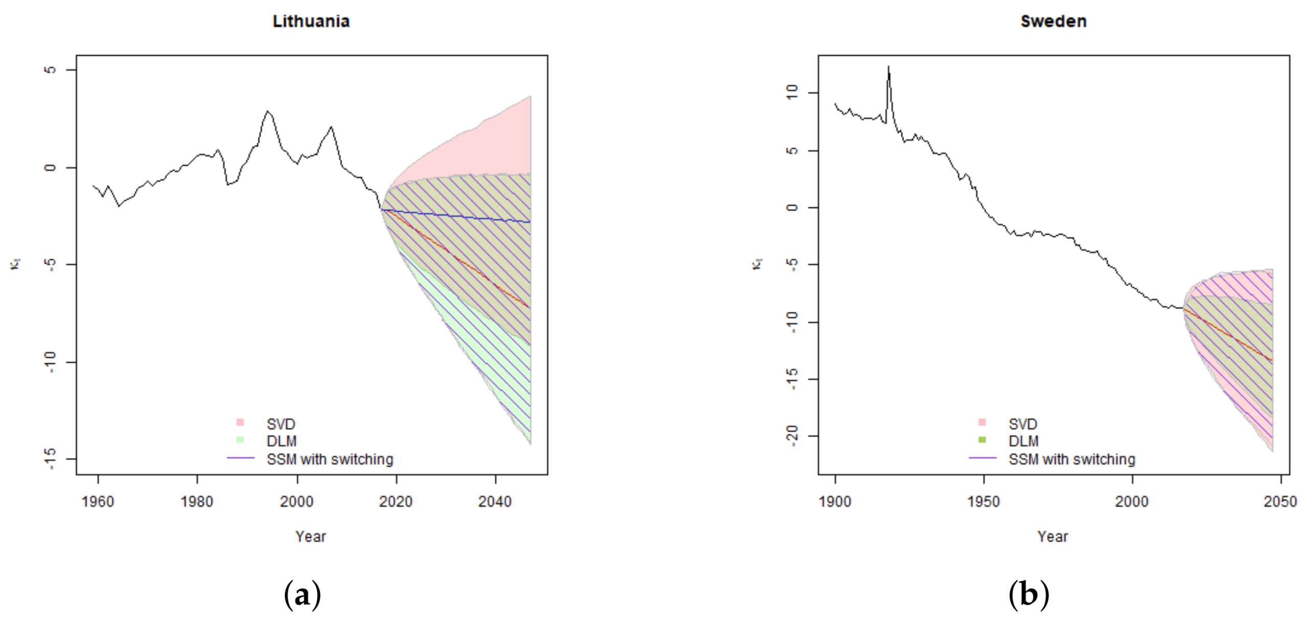
As can be seen from Equation (2), the uncertainty of the parameter ${\kappa }_t$ is driven by variation in drift parameter $\overline{\mu }$ and the residual error. The results of the simulations of ${\kappa }_t$ are provided in Figure 5 for confidence level of $95\%$, and in Figure 6 for confidence level $99.5\%$.

In the Lithuanian case, due to unsettled historic experience, the confidence intervals are wide for both SVD and state-space models. Allowance for one-time change in trend results in a more reasonable central forecast; however, it adds additional uncertainty of the second drift parameter ${\mu }^{\left(II\right)}$. Thus although estimated error variance ${\sigma }_Q^2$ is lower in SSM case, the overall confidence interval of ${\kappa }_t$ is even slightly wider than the one derived by using the classical Lee-Carter model.

In the Lithuanian case, the SSM with switching does not converge to two clearly expressed low and high variance regimes. Therefore, the distribution of error terms modelled as a mixture can be well approximated with Normal distribution. For this reason, the simulated confidence intervals for both models are very similar.

In the Swedish case, DLM gives a narrower estimate of confidence interval with respect to SVD generally due to the better fit and the lower error variance. For Sweden SSM with switching converges into two different regimes: low probability and high variance pandemic regime and high probability low variance usual development regime. Thus, the distribution of the error terms when modelled as a mixture, has much heavier tails than when it is approximated with a single Normal distribution. This results in significantly wider confidence intervals for SSM with switching, especially at 99.5% confidence level. We note that the width on the difference in confidence intervals is driven by model differences, not the poor fit. As shown in model comparison Section 4.4, despite having the widest confidence intervals SSM with switching has higher log-likelihood that DLM and is a preferred model for Sweden.

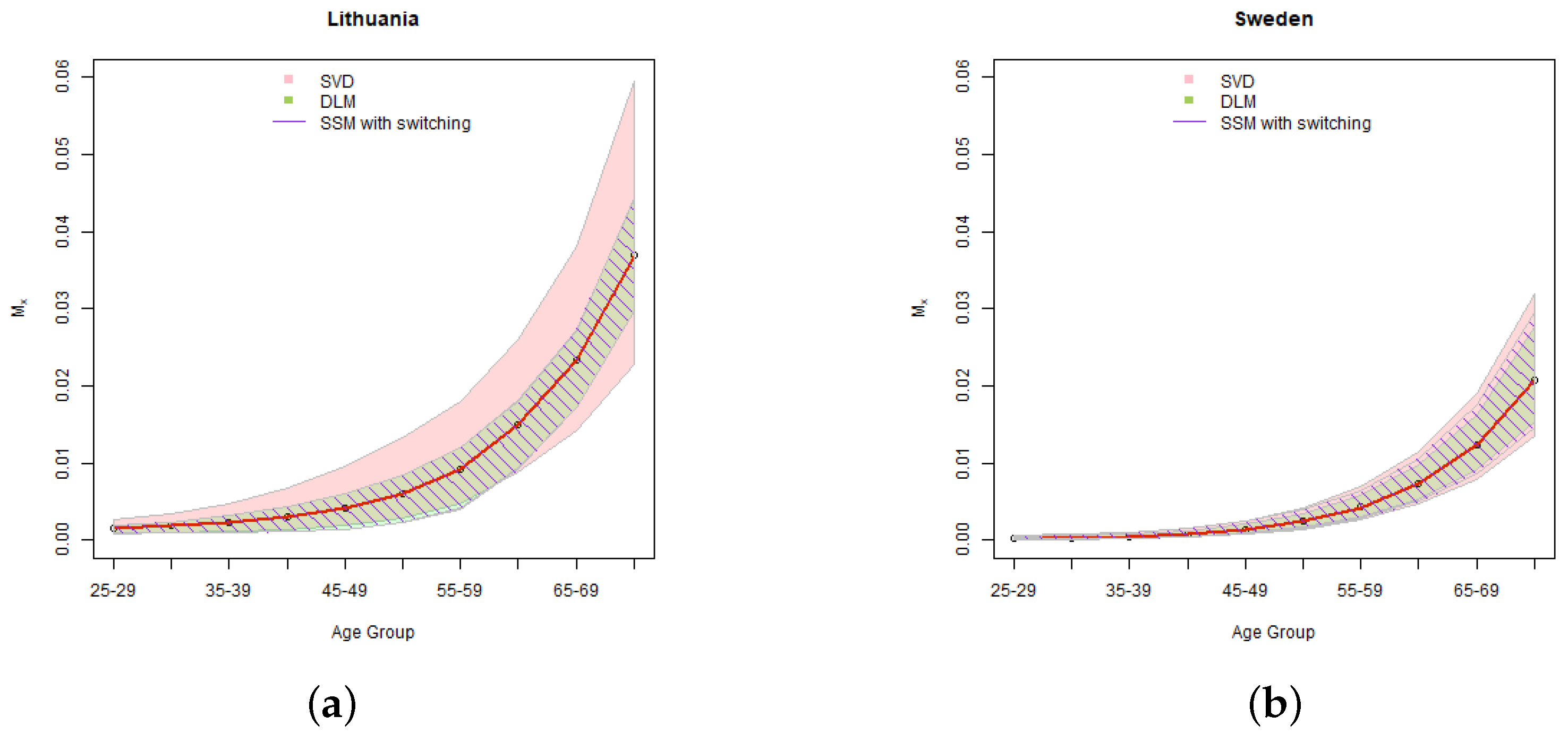
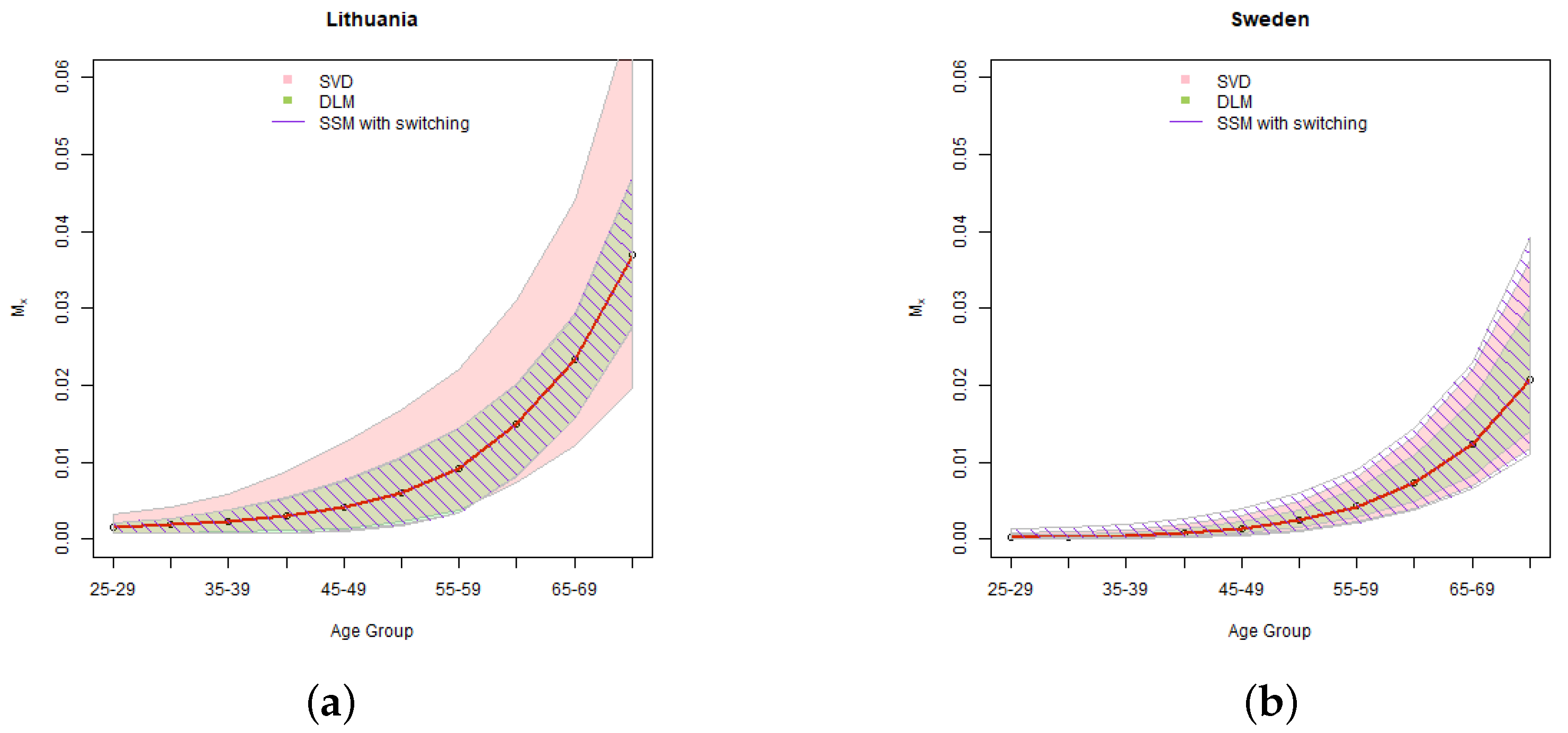
5.2. Uncertainty of Mortality Rates

The results of the simulations of $m_{x,t}$ mortality rates are provided in Figure 7 for confidence level of 95%, and Figure 8 for confidence level 99.5%. Considering that in practical applications we usually need a set of mortality rates for each of the future years in the forecasting period, in our illustration we provide the results for 15 year projection, which is in the middle of the total forecasting period.

As we can see in Equation (7), the variation in ${\kappa }_t$ is translated to changes of the mortality rates via the parameter ${\beta }_x$. The higher ${\beta }_x$ for a certain age group is, the more sensitive are the projected mortality rates of that age group to changes in ${\kappa }_t$, and vice versa. As shown in Table 3, for Lithuania the highest ${\beta }_x$ are for mid-ages and therefore in the state-space models mid-agers get the widest confidence intervals. The Lithuanian SVD calculations, due to relatively poor fit, have a large residual variance, which dominates in the classical Lee-Carter model simulations and results in very wide simulated mortality rate confidence intervals. Thus, despite we did not manage to achieve with SSMs a significant improvement in the confidence intervals of the parameter ${\kappa }_t$, the width of the simulated confidence intervals of mortality rates are reasonable and comparable to the Swedish result.

In the Swedish case, the results are consistent with the results of simulation of parameter ${\kappa }_t$. Due to better fit, at 95% confidence level the confidence intervals of SSMs are narrower than in case of SVD. At 99.5% confidence level, as expected, the heavy tails of SSMs with swithing prevail, resulting in the widest confidence intervals.

6. Discussion

Overall, the use of state-space models enabled us to achieve better fit and to derive more reasonable confidence intervals of the projected mortality rates. The methods developed in the paper can be used in common mortality modelling situations when there is a major change in mortality development trend or major fluctuations in mortality are observed. In particular, in the Swedish case the pandemic effect was well captured by SSM with switching and both DLM and SSM with switching allowed us to take into account the Lithuanian change in mortality trend. However, SSM with switching model developed in this paper proved to capture more prolonged and less sharp fluctuations in the level of mortality less successfully and further research is needed in this area.

The analysis also showed that in case of mortality projections, if we want to achieve high confidence levels, we need to accept wide confidence intervals. Historically, mortality experience was volatile, and we cannot preclude this volatility in the future. The analysis also showed that in some cases Normal approximation of the distribution of residuals, which have true mixture distribution, can unjustifiably narrow the confidence intervals of the projections, especially for high confidence levels. This could have negative implications for insurers, who use high confidence intervals in their risk and capital models as application of too narrowly distributed projections may lead to understatement of the economic capital.

The study demonstrated the advantages of SSM in the mortality modelling, in particular in ensuring higher flexibility and more coherent estimation of parameters. Overall, SSM may be used to flex other parameters of the Lee-Carter model. For example, it is possible to model the variance of residual of parameter ${\kappa }_t$ stochastically as in [12], apply regime-switching to parameter ${\beta }_x$, or apply state-space Poisson model as in Chapter 9 of [8] or introduce certain volatility of a drift of time varying index. Considering the recent developments in the area of nonlinear SSMs and sequential Monte Carlo methods the possibilities of their application in mortality studies are very high.

In practice, it also possible to use the Bayesian structure of the model. In this research, we used weakly informative priors to “let data to speak for itself”. However, in practice more informative priors are often used, to use experience from peers, introduce expected developments stemming from business plans, or simply apply the expert judgement. Thus, with SSM we can introduce not only greater flexibility of the model but also of its parameters.