Article

Total Least-Squares Collocation: An Optimal Estimation Technique for the EIV-Model with Prior Information

by
Burkhard Schaffrin
Geodetic Science Program, School of Earth Sciences, The Ohio State University, Columbus, OH 43210, USA
Mathematics 2020, 8(6), 971; https://doi.org/10.3390/math8060971
Submission received: 3 May 2020 / Revised: 31 May 2020 / Accepted: 1 June 2020 / Published: 13 June 2020
(This article belongs to the Special Issue Stochastic Models for Geodesy and Geoinformation Science)

Abstract

:
In regression analysis, oftentimes a linear (or linearized) Gauss-Markov Model (GMM) is used to describe the relationship between certain unknown parameters and measurements taken to learn about them. As soon as there are more than enough data collected to determine a unique solution for the parameters, an estimation technique needs to be applied such as ‘Least-Squares adjustment’, for instance, which turns out to be optimal under a wide range of criteria. In this context, the matrix connecting the parameters with the observations is considered fully known, and the parameter vector is considered fully unknown. This, however, is not always the reality. Therefore, two modifications of the GMM have been considered, in particular. First, ‘stochastic prior information’ (p. i.) was added on the parameters, thereby creating the – still linear – Random Effects Model (REM) where the optimal determination of the parameters (random effects) is based on ‘Least Squares collocation’, showing higher precision as long as the p. i. was adequate (Wallace test). Secondly, the coefficient matrix was allowed to contain observed elements, thus leading to the – now nonlinear – Errors-In-Variables (EIV) Model. If not using iterative linearization, the optimal estimates for the parameters would be obtained by ‘Total Least Squares adjustment’ and with generally lower, but perhaps more realistic precision. Here the two concepts are combined, thus leading to the (nonlinear) ’EIV-Model with p. i.’, where an optimal estimation (resp. prediction) technique is developed under the name of ‘Total Least-Squares collocation’. At this stage, however, the covariance matrix of the data matrix – in vector form – is still being assumed to show a Kronecker product structure.

1. Introduction

Over the last 50 years or so, the (linearized) Gauss-Markov Model (GMM) as standard model for the estimation of parameters from collected observation [1,2] has been refined in a number of ways. Two of these will be considered in more detail, namely
  • the GMM after strengthening the parameters through the introduction of “stochastic prior information”. The relevant model will be the “Random Effects Model (REM)”, and the resulting estimation technique has become known as “least-squares collocation” [3,4].
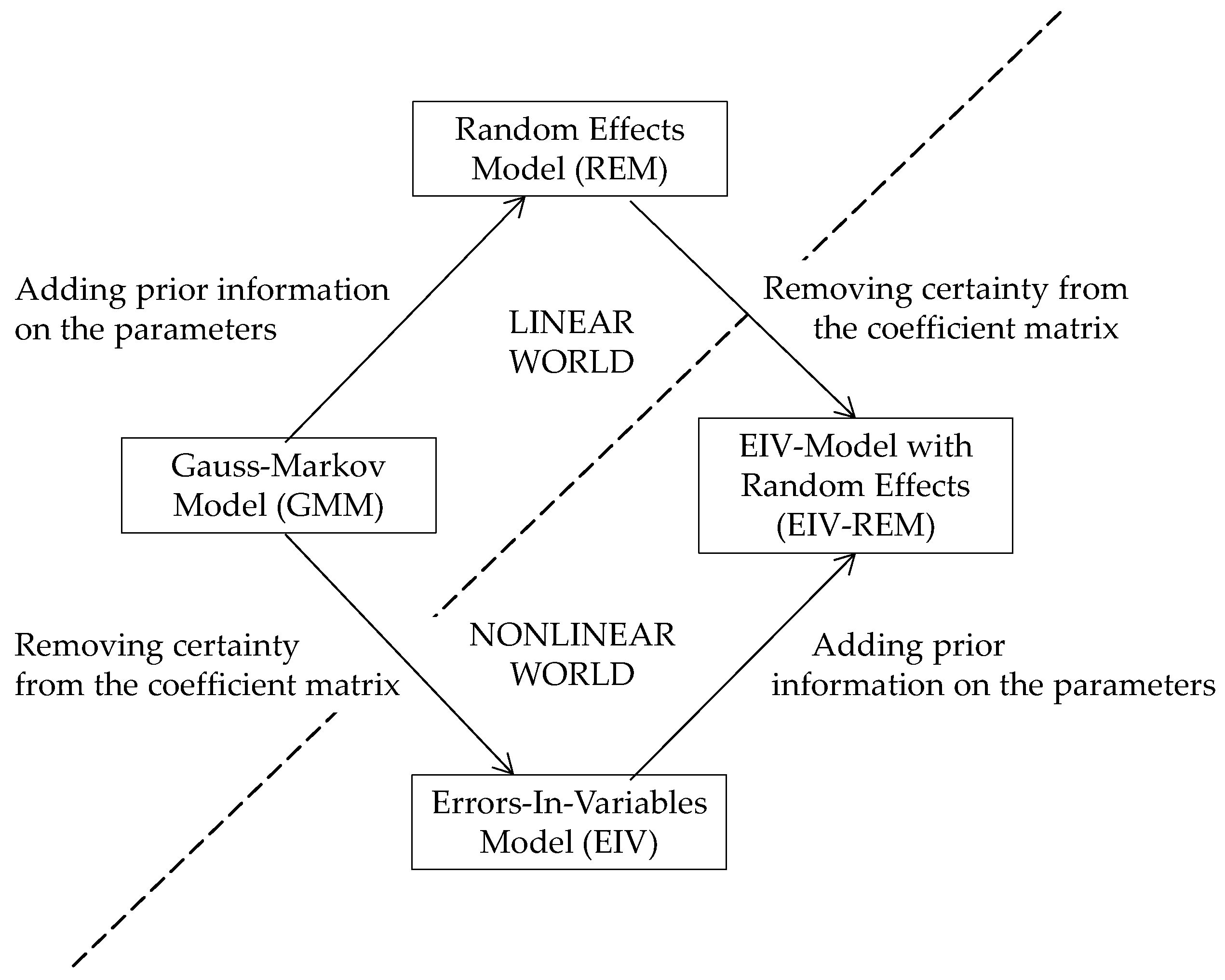
  • the GMM after weakening the coefficient matrix through the replacement of fixed entries by observed data, resulting in the (nonlinear) Errors-In-Variables (EIV) Model. When nonlinear normal equations are formed and subsequently solved by iteration, the resulting estimation technique has been termed “Total Least-Squares (TLS) estimation” [5,6,7]. The alternative approach, based on iteratively linearizing the EIV-Model, will lead to identical estimates of the parameters [8].
After a compact review and comparison of several key formulas (parameter estimates, residuals, variance component estimate, etc.) within the above three models, a new model will be introduced that allows the strengthening of the parameters and the weakening of the coefficient matrix at the same time. The corresponding estimation technique will be called “TLS collocation” and follows essentially the outline that had first been presented by this author in June 2009 at the Intl. Workshop on Matrices and Statistics in Smolenice Castle (Slovakia); cf. Schaffrin [9].
Since then, further computational progress has been made, e.g. Snow and Schaffrin [10]; but several open questions remain that need to be addressed elsewhere. These include issues related to a rigorous error propagation of the “TLS collocation” results; progress may be achieved here along similar lines as in Snow and Schaffrin [11], but is beyond the scope of the present paper.
For a general overview of the participating models, the following diagram (Figure 1) may be helpful.
The most informative model defines the top position, and the least informative model is at the bottom. The new model can be formed at the intermediate level (like the GMM), but belongs to the “nonlinear world” where nonlinear normal equations need to be formed and subsequently solved by iteration.

2. A Compact Review of the “Linear World”

2.1. The (linearized) Gauss-Markov Model (GMM)

Let the Gauss-Markov Model be defined by
y = A n × m ξ + e   , q : = rk   A min   { m , n }   , e ( 0 , σ 0 2 I n )   ,
possibly after linearization and homogeneization; cf. Koch [2], or Grafarend and Schaffrin [12] among many others.
Here, y denotes the n × 1 vector of (incremental) observations,
A
the n × m matrix of coefficients (given),
ξ
the m × 1 vector of (incremental) parameters (unknown),
e
the n × 1 vector of random errors (unknown) with expectation E { e } = 0 while the dispersion matrix D { e } = σ 0 2 I n is split into the (unknown) factor
σ 0 2
as variance component (unit-free) and
I n
as (homogeneized) n × n symmetric and positive-definite “cofactor matrix” whose inverse is better known as “weight matrix” P ; here P = I n for the sake of simplicity.
Now, it is well known that the Least-Squares Solution (LESS) is based on the principle
e T e = min   s . t . e = y A   ξ
which leads to the “normal equations”
N   ξ ^ = c   for [ N ,   c ] : = A T [ A ,   y ] .
Depending on rk N, the rank of the matrix N, the LESS may turn out uniquely as
ξ ^ LESS = N 1 c   iff rk   N = rk   A = q = m ;
or it may belong to a solution (hyper)space that can be characterized by certain generalized inverses of N, namely
ξ ^ LESS { N c | N   N N = N } = = { N r s c | N   N r s N = N   ,   N r s N   N r s = N r s = ( N r s ) T }   ;
where N r s denotes an arbitrary reflexive symmetric g-inverse of N (including the “pseudo-inverse” N + ),
iff rk   N = rk   A = q < m .
In the latter case (6), any LESS will be biased with
bias   ( ξ ^ LESS ) = E { ξ ^ LESS ξ } { ( I m N N )   ξ } = { ( I m N r s N )   ξ } ,
its dispersion matrix will be
D   { ξ ^ LESS } = σ 0 2 N N ( N ) T { σ 0 2 N r s | N   N r s N = N ,   N r s N   N r s = N r s = ( N r s ) T } ,
and its Mean Squared Error (MSE) matrix, therefore,
M S E   { ξ ^ LESS } { σ 0 2 [ N r s + ( I m   N r s N ) ( ξ   σ 0 2 ξ T ) ( I m N r s N ) T ] } .
In contrast to the choice of LESS in case (6), the residual vector will be unique; for any ξ ^ LESS :
e ˜ LESS = y A   ξ ^ LESS         ( 0 ,   σ 0 2 ( I n A   N r s A T ) = D { y } D { A   ξ ^ LESS } ) .
Hence, the optimal variance component estimate will also be unique:
σ ^ 0 2 = ( n q ) 1 e ˜ LESS T e ˜ LESS = ( n q ) 1 ( y T y c T ξ ^ LESS ) ,
E { σ ^ 0 2 } = σ 0 2   ,   D { σ ^ 0 2 } 2 ( σ 0 2 ) 2 / ( n q )     under   quasi-normality .
For the corresponding formulas in the full-rank case (4), the reflexive symmetric g-inverse N r s simply needs to be replaced by the regular inverse N 1 , thereby showing that the LESS turns into an unbiased estimate of ξ while its MSE-matrix coincides with its dispersion matrix (accuracy precision).

2.2. The Random Effects Model (REM)

Now, additional prior information (p. i.) is introduced to strengthen the parameter vector within the GMM (1). Based on Harville’s [13] notation of a m × 1 vector 0 ~ of so-called “pseudo-observations”, the new m × 1 vector
x : = ξ 0 ~ of   random   effects   ( unknown )   is   formed   with
E { x } = β 0 as   given   m × 1   vector   of   p .   i .   and
D { x } = σ 0 2 Q 0 as   n × n   positive-(semi)definite   dispersion   matrix   of   the   p .   i .
Consequently, the Random Effects Model (REM) can be stated as
y ~ : = y A 0 ~ = A n × m x + e   , q : = rk   A min { m , n }   , β 0 m × 1 : = x + e 0 ,
[ e e 0 ] (   [ 0 0 ]   ,   σ 0 2 [ I n 0 0 Q 0 ]   )   , Q 0 m × m   symmetric   and   nnd   ( non-negative   definite ) .
If P 0 : = Q 0 1 exists, the estimation/prediction of x may now be based on the principle
e T e + e 0 T P 0   e 0 = min s . t . e = y ~ A x   , e 0 = β 0 x ,
which leads to the “normal equations” for the “Least-Squares Collocation (LSC)” solution
( N + P 0 ) x ˜ = c ~   + P 0 β 0
which is unique even in the rank-deficient case (6).
If Q 0 is singular, but e 0 ( Q 0 ) with probability 1, then there must exist an m × 1 vector ν 0 with
Q 0   ν 0 = e 0 = x β 0 with   probability   1     ( a . s . almost   surely ) .
Thus, the principle (18) may be equivalently replaced by
e T e + ( ν 0 ) T Q 0   ν 0 = min s . t . e = y ~ A x     and   ( 20 ) ,
which generates the LSC solution uniquely from the “modified normal equations”
  ( I m + Q 0 N ) x ˜ LSC = β 0 + Q 0 c ~     for   c ~ : = A T y ~
or, alternatively, via the “update formula
  x ˜ LSC = β 0 + Q 0   ( I m + N Q 0 ) 1 ( c ~ N β 0 )  
which exhibits the “weak (local) unbiasedness” of x ˜ LSC via
E { x ˜ LSC } = β 0 + Q 0   ( I m + N Q 0 ) 1 ( E { c ~ } N β 0 ) = β 0 + 0 = E { x } .
Consequently, the MSE-matrix of x ˜ LSC can be obtained from
M S E   { x ˜ LSC } = D   { x ˜ LSC x } = σ 0 2 Q 0   ( I m + N Q 0 ) 1 =
= σ 0 2   ( N + P 0 ) 1 if P 0 : = Q 0 1   exists ,
whereas the dispersion matrix of x ˜ LSC itself is of no relevance here. It holds:
D { x ˜ LSC } = D   { x } D   { x x ˜ LSC } = σ 0 2 Q 0   σ 0 2 Q 0 ( I m + N Q 0 ) 1 .
Again, both residual vectors are uniquely determined from
( e ˜ 0 ) LSC = β 0 x ˜ LSC = Q 0   ν ^ LSC 0 for
ν ^ LSC 0 : = ( I m + N Q 0 ) 1 ( c ~   N β 0 ) ,   and
e ˜ LSC = y ~   A   x ˜ LSC = [ I m A   Q 0 ( I m + N Q 0 ) 1 A T ]   ( y ~   A β 0 )
with the control formula
  A T e ˜ L S C = ν ^ LSC 0     .
An optimal estimate of the variance component may now be obtained from
( σ ^ 0 2 ) LSC = n 1 ( e ˜ LSC T e ˜ LSC + ( ν ^ LSC 0 ) T Q 0   ν ^ LSC 0 ) = = n 1 ( y ~ T y ~     c ~ T x ˜ LSC β 0 T ν ^ LSC 0 )   .

3. An Extension into the “Nonlinear World”

3.1. The Errors-In-Variables (EIV) Model

In this scenario, the Gauss-Markov Model (GMM) is further weakened by allowing some or all of the entries in the coefficient matrix A to be observed. So, after introducing a corresponding n × m matrix of unknown random errors E A , the original GMM (1) turns into the EIV-Model
y = ( A E A ) n × m ξ + e   , q : = rk   A = m < n   , e ( 0 , σ 0 2 I n )   ,
with the vectorized form of E A being characterized through
e A n m × 1 : = vec   E A ( 0 , σ 0 2 ( I m I n ) = σ 0 2 I m n )   , C { e , e A } = 0     ( assumed ) .
Here, the vec operation transform a matrix into a vector by stacking all columns underneath each other while denotes the Kronecker-Zehfuss product of matrices, defined by
G p × q H r × s = [ g i j H ] p r × q s if G = [ g i j ] .
In particular, the following key formula holds true:
vec   ( A   B   C T ) = ( C A ) vec   B
for matrices of suitable size. Note that, in (34), the choice Q A : = I m n is a very special one. In general, Q A may turn out singular whenever some parts of the matrix A remain unobserved (i.e., nonrandom).
In any case, thanks to the term
E A ξ = ( ξ T I n )   e A ,
the model (33) needs to be treated in the “nonlinear world” even though the vector ξ may contain only incremental parameters. From now on, A is assumed to have full column rank, rk   A = : q = m .
Following Schaffrin and Wieser [7], for instance, the “Total-Least Squares Solution (TLSS)” can be based on the principle
e T e + e A T e A = min s . t . ( 33 - 34 ) ,
and the Lagrange function
Φ   ( e , e A , ξ , λ ) : = e T e + e A T e A + 2 λ T ( y A   ξ e + E A ξ ) = = e T e + e A T e A + 2 λ T [ y A   ξ e + ( ξ T I n )   e A ]
which needs to be made stationary. The necessary Euler-Lagrange conditions then read:
1 2   Φ   e = e ˜ λ ^ 0 λ ^ = e ˜
1 2   Φ   e A = e ˜ A + ( ξ ^ TLS I n )   λ ^ 0 E ˜ A = λ ^   ξ ^ TLS T
1 2   Φ   ξ = ( A E ˜ A ) T λ ^ 0 A T λ ^ = E ˜ A T λ ^ = ξ ^ TLS ( λ ^ T λ ^ )
1 2   Φ   λ = y A   ξ ^ TLS e ˜ + E ˜ A   ξ ^ TLS 0 y A   ξ ^ TLS = λ ^   ( 1 + ξ ^ TLS T   ξ ^ TLS )
c N ξ ^ TLS : = A T ( y A   ξ ^ TLS ) = A T λ ^   ( 1 + ξ ^ TLS T   ξ ^ TLS ) = ξ ^ TLS ν ^ TLS
for
ν ^ TLS : = ( λ ^ T λ ^ ) ( 1 + ξ ^ TLS T   ξ ^ TLS ) = λ ^ T ( y A   ξ ^ TLS ) =
= ( 1 + ξ ^ TLS T   ξ ^ TLS ) 1 ( y A   ξ ^ TLS ) T ( y A   ξ ^ TLS ) =
= ( 1 + ξ ^ TLS T   ξ ^ TLS ) 1   [ y T ( y A   ξ ^ TLS ) ξ ^ TLS T   ( c N   ξ ^ TLS ) ]         0
( 1 + ξ ^ TLS T   ξ ^ TLS ) ν ^ TLS = y T y c T ξ ^ TLS + ( ξ ^ TLS T   ξ ^ TLS ) ν ^ TLS
    ν ^ TLS = y T y c T ξ ^ TLS  
which needs to be solved in connection with the “modified normal equations” from (44), namely
  ( N ν ^ TLS I m )   ξ ^ TLS = c     .
Due to the nonlinear nature of ξ ^ TLS , it is not so easy to determine if it is an unbiased estimate, or how its MSE-matrix may exactly look like. First attempts of a rigorous error propagation have recently been undertaken by Amiri-Simkooei et al. [14] and by Schaffrin and Snow [15], but are beyond the scope of this paper.
Instead, both the optimal residual vector e ˜ TLS and the optimal residual matrix ( E ˜ A ) TLS are readily available through (40) and (43) as
e ˜ TLS = λ ^ = ( y A   ξ ^ TLS ) ( 1 + ξ ^ TLS T   ξ ^ TLS ) 1 ,
and through (41) as
( E ˜ A ) TLS = e ˜ TLS ξ ^ TLS T = ( y A   ξ ^ TLS ) ( 1 + ξ ^ TLS T   ξ ^ TLS ) 1 ξ ^ TLS .
As optimal variance component estimate, it is now proposed to use the formula
( σ ^ 0 2 ) TLS = ( n m ) 1 [   e ˜ TLS T   e ˜ TLS + ( e ˜ A ) TLS T   ( e ˜ A ) TLS ] =
  = ( n m ) 1 λ ^ T λ ^ ( 1 + ξ ^ TLS T   ξ ^ TLS ) = ν ^ TLS / ( n m ) ,
in analogy to the previous estimates (11) and (32).

3.2. A New Model: The EIV-Model with Random Effects (EIV-REM)

In the following, the above EIV-Model (33-34) is strengthened by introducing stochastic prior information (p. i.) on the parameters which thereby change their character and become “random effects” as in (13-15). The EIV-REM can, therefore, be stated as
y ~ = ( A E A ) n × m x + e   , q : = rk   A min { m , n }   , β 0 = x + e 0   ( given ) ,
with
[ e e A = vec   E A e 0 ]         (   [ 0 0 0 ]   ,   σ 0 2 [ I n 0 0 0 I m n 0 0 0 Q 0 ]   )   ,     Q 0   symmetric   and   nnd .
The first set of formulas will be derived by assuming that the weight matrix P 0 : = Q 0 1 exists uniquely for the p. i. Then, the “TLS collocation (TLSC)” may be based on the principle
e T e + e A T e A + e 0 T P 0   e 0 = min s . t . ( 53 - 54 ) ,
resp. on the Lagrange function
Φ   ( e , e A , e 0 , λ ) : = e T e + e A T e A + e 0 T P 0   e 0 + 2 λ T [ ( y ~   A   β 0 e + ( β 0 T I n )   e A + A   e 0 E A   e 0 = ( e 0 T   I n ) e A ]
which needs to be made stationary. The necessary Euler-Lagrange conditions then read:
1 2   Φ   e = e ˜ λ ^ 0 λ ^ = e ˜
1 2   Φ   e A = e ˜ A + [ ( β 0 e ˜ 0 ) I n ]   λ ^ 0 E ˜ A = λ ^ ( β 0 e ˜ 0 ) T = : λ ^   x ˜ TLSC T
1 2   Φ   e 0 = P 0   e ˜ 0 + ( A E ˜ A ) T λ ^ 0 A T λ ^ = E ˜ A T λ ^ P 0   e ˜ 0
A T λ ^ = x ˜ TLSC ( λ ^ T λ ^ ) + ν ^ TLSC 0 for ν ^ TLSC 0 : = P 0   e ˜ 0 = P 0 ( β 0 x ˜ TLSC )
1 2   Φ   λ = y ~ A   ( β 0 e ˜ 0 ) e ˜ + E ˜ A   ( β 0 e ˜ 0 ) 0 y ~   A   x ˜ TLSC = λ ^   ( 1 + x ˜ TLSC T   x ˜ TLSC )
λ ^ = ( y ~ A   x ˜ TLSC ) ( 1 + x ˜ TLSC T   x ˜ TLSC ) 1 .
Combining (60) with (62) results in
( c ~ N   x ˜ TLSC ) ( 1 + x ˜ TLSC T   x ˜ TLSC ) 1 = A T λ ^ = x ˜ TLSC ( 1 + x ˜ TLSC T   x ˜ TLSC ) 2 ( y ~   A   x ˜ TLSC ) T ( y ~   A   x ˜ TLSC ) + ν ^ TLSC 0 ,
and finally in
  ( N + ( 1 + x ˜ TLSC T   x ˜ TLSC ) P 0 ν ^ TLSC I m )   x ˜ TLSC = c ~   + P 0   β 0 ( 1 + x ˜ TLSC T   x ˜ TLSC )  
where
  ν ^ TLSC : = ( 1 + x ˜ TLSC T   x ˜ TLSC ) 1 ( y ~   A   x ˜ TLSC ) T ( y ~   A   x ˜ TLSC )   ,   and   ν ^ TLSC 0 : = P 0   ( β 0 x ˜ TLSC ) = P 0   e ˜ 0   ,   provided   that   P 0   exists   .
In the more general case of a singular matrix Q 0 , an approach similar to (20) can be followed, leading to the equation system
  [ ( 1 + x ˜ TLSC T   x ˜ TLSC ) I m + Q 0 N ν ^ TLSC Q 0 ]   x ˜ TLSC = β 0 ( 1 + x ˜ TLSC T   x ˜ TLSC ) + Q 0 c ~  
that needs to be solved in connection with (65). Obviously,
  x ˜ TLSC   β 0   if Q 0 0   , and     x ˜ TLSC     x ˜ TLS   if P 0   0   .
Again, it is still unclear if x ˜ TLSC represents an unbiased prediction of the vector x of random effects. Also, very little (if anything) is known about the corresponding MSE-matrix of x ˜ TLSC . The answers to these open problems will be left for a future contribution. It is, however, possible to find the respective residual vectors/matrices represented as follows:
e ˜ TLSC = λ ^ = ( y ~ A   x ˜ TLSC ) ( 1 + x ˜ TLSC T   x ˜ TLSC ) 1 ,
( E ˜ A ) TLSC = λ ^ x ˜ TLSC T = ( y ~   A   x ˜ TLSC ) ( 1 + x ˜ TLSC T   x ˜ TLSC ) 1 x ˜ TLSC T ,
( e ˜ 0 ) TLSC = Q 0 ν ^ TLSC 0 = β 0   x ˜ TLSC ,
while a suitable formula for the variance component is suggested as
( σ ^ 0 2 ) TLSC = n 1     [   ν ^ TLSC + ( ν ^ TLSC 0 ) T Q 0   ( ν ^ TLSC 0 ) ] .

4. Conclusions and Outlook

Key formulas have been developed successfully to optimally determine the parameters and residuals within the new ‘EIV-Model with p. i.’ (or EIV-REM) which turns out to be more general than the other three models considered here (GMM, REM, EIV-Model). In particular, it is quite obvious that
  • EIV-REM becomes the REM if D { e A } : = 0 ,
  • EIV-REM becomes the EIV-Model if P 0 : = 0 ,
  • EIV-REM becomes the GMM if both P 0 : = 0 and D { e A } : = 0 .
Hence the new EIV-REM can indeed serve as a universal representative of the whole class of models presented here.
Therefore, in a follow-up paper, it is planned to also cover more general dispersion matrices for e and e A in (54), similarly to the work by Schaffrin et al. [16] for the EIV-Model with singular dispersion matrices for e A .

Funding

This research received no external funding.

Conflicts of Interest

The author declares no conflict of interest.

References

  1. Rao, C.R. Estimation of parameters in a linear model. Ann. Statist. 1976, 4, 1023–1037. [Google Scholar] [CrossRef]
  2. Koch, K.-R. Parameter Estimation and Hypothesis Testing in Linear Models; Springer: Berlin/Heidelberg, Germany, 1999; p. 334. [Google Scholar]
  3. Moritz, H. A generalized least-squares model. Studia Geophys. Geodaet. 1970, 14, 353–362. [Google Scholar] [CrossRef]
  4. Schaffrin, B. Model Choice and Adjustment Techniques in the Presence of Prior Information; Technical Report No. 351; The Ohio State University Department of Geodetic Science and Survey: Columbus, OH, USA, 1983; p. 37. [Google Scholar]
  5. Golub, G.H.; van Loan, C.F. An analysis of the Total Least-Squares problem. SIAM J. Numer. Anal. 1980, 17, 883–893. [Google Scholar] [CrossRef]
  6. Van Huffel, S.; Vandewalle, J. The Total Least-Squares Problem: Computational Aspects and Analysis; SIAM: Philadelphia, PA, USA, 1991; p. 300. [Google Scholar]
  7. Schaffrin, B.; Wieser, A. On weighted Total Least-Squares adjustment for linear regression. J. Geod. 2008, 82, 415–421. [Google Scholar] [CrossRef]
  8. Schaffrin, B. Adjusting the Errors-In-Variables model: Linearized Least-Squares vs. nonlinear Total Least-Squares procedures. In VIII Hotine-Marussi Symposium on Mathematical Geodesy; Sneeuw, N., Novák, P., Crespi, M., Sansó, F., Eds.; Springer International Publishing: Cham, Switzerland, 2015; pp. 301–307. [Google Scholar]
  9. Schaffrin, B. Total Least-Squares Collocation: The Total Least-Squares approach to EIV-Models with prior information. In Proceedings of the 18th International Workshop on Matrices and Statistics, Smolenice Castle, Slovakia, 23–27 June 2009. [Google Scholar]
  10. Snow, K.; Schaffrin, B. Weighted Total Least-Squares Collocation with geodetic applications. In Proceedings of the SIAM Conference on Applied Linear Algebra, Valencia, Spain, 18–22 June 2012. [Google Scholar]
  11. Schaffrin, B.; Snow, K. Progress towards a rigorous error propagation for Total Least-Squares estimates. J. Appl. Geod. 2020. accepted for publication. [Google Scholar] [CrossRef]
  12. Grafarend, E.; Schaffrin, B. Adjustment Computations in Linear Models; Bibliographisches Institut: Mannheim, Germany; Wiesbaden, Germany, 1993; p. 483. (In German) [Google Scholar]
  13. Harville, D.A. Using ordinary least-squares software to compute combined intra-interblock estimates of treatment contrasts. Am. Stat. 1986, 40, 153–157. [Google Scholar]
  14. Amiri-Simkooei, A.R.; Zangeneh-Nejad, F.; Asgari, J. On the covariance matrix of weighted Total Least-Squares estimates. J. Surv. Eng. 2016, 142. [Google Scholar] [CrossRef] [Green Version]
  15. Schaffrin, B.; Snow, K. Towards a more rigorous error propagation within the Errors-In-Variables Model for applications in geodetic networks. In Proceedings of the 4th Joint International Symposium on Deformation Monitoring (JISDM 2019), Athens, Greece, 15–17 May 2019. electronic proceedings only. [Google Scholar]
  16. Schaffrin, B.; Snow, K.; Neitzel, F. On the Errors-In-Variables Model with singular dispersion matrices. J. Geod. Sci. 2014, 4, 28–36. [Google Scholar] [CrossRef]
Figure 1. Model Diagram.
Mathematics 08 00971 g001

