Performance Evaluation of Deep Learning-Based Gated Recurrent Units (GRUs) and Tree-Based Models for Estimating ETo by Using Limited Meteorological Variables

Abstract

The amount of water allocated to irrigation systems is significantly greater than the amount allocated to other sectors. Thus, irrigation water demand management is at the center of the attention of the Ministry of Agriculture and Forestry in Turkey. To plan more effective irrigation systems in agriculture, it is necessary to accurately calculate plant water requirements. In this study, daily reference evapotranspiration (ETo) values were estimated using tree-based regression and deep learning-based gated recurrent unit (GRU) models. For this purpose, 15 input scenarios, consisting of meteorological variables including maximum and minimum temperature, wind speed, maximum and minimum relative humidity, dew point temperature, and sunshine duration, were considered. ETo values calculated according to the United Nations Food and Agriculture Organization (FAO) Penman-Monteith method were considered as model outputs. The results indicate that the random forest model, with a correlation coefficient of 0.9926, is better than the other tree-based models. In addition, the GRU model, with R = 0.9837, presents good performance relative to the other models. In this study, it was found that maximum temperature was more effective in estimating ETo than other variables.

1. Introduction

Today, with a growing population, reliable food production and supply are among the main policy concerns of many countries, highlighting the need to use renewable water efficiently to prevent future water shortages. In Turkey, the amount of water allocated to agriculture is significantly greater than for other sectors; thus, the careful use of water is important. To plan irrigation networks and to save water, the water needs of different agricultural plants should be determined correctly [1]. There are various methods to determine plant water requirements, but the Penman-Monteith (ETo-PM) method presented by the United Nations Food and Agriculture Organization (FAO) has been accepted as the standard, since other methods give different results [2]. This method calculates reference evapotranspiration values using different meteorological variables.

Developments in technology have made it possible to measure increasing amounts of data. In data mining, data is first stored digitally, and then automatically searched by a machine. Data mining is an area that concerns learning in a practical, nontheoretical sense. The methods used in data-based models find hidden information and patterns in the data and make predictions. This technique is receiving significant attention, having been recognized as a newly emerging tool for analysis [3]. Many experiences of applying machine learning to data mining indicate that clear information structures and the acquisition of structural definitions are as important as the ability to perform well on new examples. Machine learning algorithms are a form of artificial intelligence, but different researchers have expressed this concept in various terms. However, according to all authors, the purpose of machine learning techniques is to make predictions by training data with a machine [4]. Researchers often use data mining not only for predictions, but also for obtaining or extracting information.

Recently, artificial intelligence—specifically, machine learning and data mining—has been used to calculate evapotranspiration (ETo) amounts. Pal and Desval [5] used meteorological parameters as inputs in their study and estimated the amount of ETo with the M5 model at the Davis station maintained by the California Irrigation Management Information System (CIMIS). The results showed that the M5 model is suitable. Sattari et al. [6] estimated the ETo amounts for an Ankara (Turkey) station with the help of meteorological variables and a backpropagation neural network and M5 tree-based models. Although the results indicated that the Artificial Neural Networks (ANN) model gave better results, the use of the M5 model was recommended because of its simplicity and applicability. Esmailzdeh and Sattari [7] estimated the monthly ETo amount for Tabriz using multilayer perceptron (MLP), feed-forward back propagation neural networks, and genetic programming (GEP). Ten different meteorological parameters were used as input data. According to the results, both models were acceptable, but the results of the GEP method were easier to interpret and more practical. Rahimikhoob [8] used 663 NOAA-AVHRR level 1b images during the 1999–2009 period of five irrigated units used to cultivate sugar cane, located in the Khuzestan plain in the southwest of Iran, to estimate ETo by employing the M5 model tree and ANN. The study showed that the estimation of ETo through the use of the M5 model tree gave better results than the ANN technique. Feng et al. [9] estimated daily ETo amounts using random forest (RF) and generalized regression neural network (GRNN) methods using meteorological parameters for southwestern China for 2009–2014. Although it was concluded that both methods were acceptable, the RF method was found to be better. Shiri [10] estimated the amount of ETo by the coupled wavelet-random forest (WRF) method according to meteorological variables. It was concluded that the results improved with the use of the WRF hybrid model. Fan et al. [11] studied the potential of a gradient boosting decision tree (GBDT), extreme gradient boosting (XGBoost), RF, and M5 model tree (M5Tree) for daily ETo modeling with limited meteorological data using a K-fold cross-validation approach. In addition, the authors used extreme learning machine (ELM) and support vector machine (SVM) models to compare the results. They used meteorological variables for 1961–2010 from weather stations in China across different climates to evaluate the models. They recommended GBDT and the XGBoost models for the estimation of ETo in different climatic conditions of China. Artificial intelligence methods with deep learning have been used not only in water engineering, but also in other branches of science, for example, for bending analysis of a Kirchhoff plate [12] or in the solution of quadratic boundary value problems [13]. Granata [14] estimated the actual amount of evapotranspiration using meteorological data from central Florida, USA, with a humid subtropical climate and four different machine learning methods (bagging, RF, M5P regression tree, and support vector regression) and compared the results. The study showed that the best results were obtained when the M5P model used meteorological parameters and the moisture content of the soil. Wang et al. [15] estimated the amount of ETo using the RF and GEP models using meteorological data from the Karst region in southwest China. According to the results, RF-based models gave better results, but GEP-based models were recommended because they provided understandable equations and were easy to use. In a review study conducted by Chia et al. [16], the authors recently evaluated the performance of hybrid-focused artificial intelligence models for ETo estimation. Within the scope of the study, models based on artificial intelligence methods were found to be successful for ETo estimation. Srivastava et al. [17] successfully estimated the amount of reference evapotranspiration (ETo) using NASA/POWER and National Center for Environmental Prediction (NCEP) global data through the Weather Research and Forecast (WRF) model for an agricultural field in northern India.

The study aims to estimate daily reference evapotranspiration values with the GRU method, which is a deep learning technique, and well-known tree regression-based models, namely, M5P, RF, random tree (RT) and RepTree methods, based on data using the measured values from the meteorology station in Tekirdağ, Turkey, which is surrounded by sea on three sides. In addition, by comparing the obtained results, the aim was to determine the model that gives the best result, and to determine the meteorological variables that are effective in the modeling and are able to make predictions with the fewest parameters.

2. Material and Methods

The Tekirdağ region is an important agricultural land of Turkey surrounded by seas. A map of this region is given in Figure 1. Among the most widely cultivated field crops in the province are wheat, sunflower, barley, corn, and alfalfa, which are produced in a total of 3,846,960 da areas. The size of the fruit production area is 109,135 da, in which grapes, apples, olives, pears, and cherries are mostly grown. Vegetables such as watermelon, melon, tomato, onion, and cucumber are produced in a total area of 43,873 da. Tekirdag province produces 10% of the total textiles, 25% of the total margarine, and 20% of the total sunflower oil of the entire country. It ranks 9th according to the socio-economic development index [18,19].

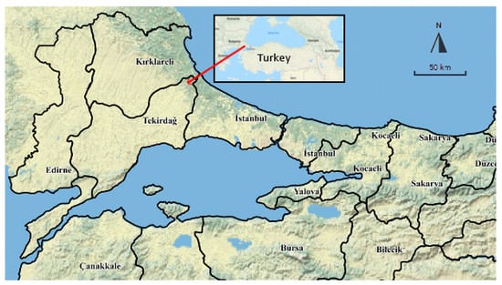
Figure 1. The study area [20].

The daily meteorological data used in the study were obtained from the State Meteorology Service. The data set consists of daily min–max temperatures, wind speeds, dew point temperatures, sunshine times, and min–max relative humidities from 1 January 1993 to 31 December 2018. The long-term monthly changes of some meteorological parameters are given in Figure 2. The statistical features of the meteorological parameters of the Tekirdag synoptic station are given in Table 1. A correlation matrix is given in Table 2 to determine the meteorological variables that have a statistically significant effect on ETo. As can be understood from the correlation matrix values, there is a strong and statistically significant relationship between the Tmax and Tmin variables and ETo amounts. In the light of the correlation values, the combinations of variables that will enter the models as input are determined.

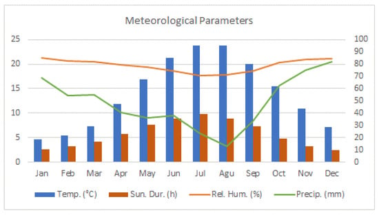
Figure 2. Selected meteorological parameters (1939 to 2018).

Table 1. Statistical features of meteorological parameters.

Variable	Minimum	Maximum	Mean	Std. Deviation
Tmin (°C)	−11.50	26.20	10.96	7.18
Tmax (°C)	−7.20	40.20	18.58	8.15
Wind speed - U2 (m/s)	0.10	10.60	2.54	1.07
Tdew (°C)	−13.15	27.07	10.79	6.92
Sunshine duration - n (hr)	0.00	11.00	5.85	2.81
Min RH (%)	1.00	100.00	65.88	16.39
Max RH (%)	37.00	100.00	88.49	8.74
ETo-PM (mm/day)	0.22	8.17	2.69	1.74

Table 2. The correlation matrix of the meteorological variables *.

Variables	MTI	tmin	tmax	u2	tdew	n	Min RH	Max RH	ETo-PM
MTI **	1	0.307	0.281	0.029	0.308	0.023	−0.038	−0.044	0.058
tmin	0.307	1	0.952	0.028	0.960	0.746	−0.336	−0.210	0.843
tmax	0.281	0.952	1	0.000	0.928	0.776	−0.455	−0.262	0.870
u2	0.029	0.028	0.000	1	−0.048	−0.032	−0.231	−0.156	0.101
tdew	0.308	0.960	0.928	−0.048	1	0.699	−0.171	−0.008	0.752
n	0.023	0.746	0.776	−0.032	0.699	1	−0.385	−0.355	0.904
Min RH	−0.038	−0.336	−0.455	−0.231	−0.171	−0.385	1	0.548	−0.550
Max RH	−0.044	−0.210	−0.262	−0.156	−0.008	−0.355	0.548	1	−0.460
ETo-PM	0.058	0.843	0.870	0.101	0.752	0.904	−0.550	−0.460	1

* Values in bold are different from 0 with a significance level alpha = 0.05; ** MTI: monthly time index.

Figure 3 indicates the distribution of the meteorological data. Tmin, Tmax, and ETo values show a distribution close to normal. Although data mining and artificial intelligence studies do not require compliance with normal distribution, it is a positive situation for the classification models to yield a successful result.

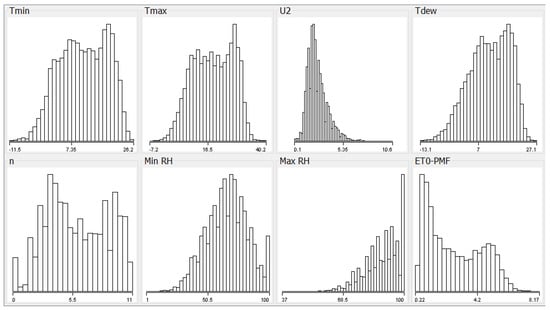
Figure 3. The distribution of the meteorological data used in the study.

2.1. ETo Calculation

FAO has defined the term ETo [21,22]. Despite the fact that the Penman-Monteith (PM) formula is much more complex than other formulas, it has been formally explained and recommended by FAO. In previous studies, the FAO Penman-Monteith equation (ETo-PM, Equation (1)) was used as a base model. The relation has two main features: (1) it can be used in any weather conditions without regional calibration, and (2) the precision of the relationship is based on lysimetric data in an approved spherical range. However, in many countries, there is still no equipment to observe these variables correctly, or data is not regularly recorded [23].

$$ETo=\frac{0.408 ∆ \left(R_n-G\right)+\gamma \frac{900}{T+273}{u}_2\left(e_s-e_a\right)}{∆+\gamma \left(1+0.34u_2\right)}$$

(1)

where ETo is reference evapotranspiration [mm day⁻¹], Rn is net radiation at the crop surface [MJ m⁻² day⁻¹], G is soil heat flux density [MJ m⁻² day⁻¹], T is the mean daily air temperature at 2 m [°C], u₂ is the wind speed at 2 m [m s⁻¹], e_s is the saturation vapour pressure [kPa], e_a is the actual vapour pressure [kPa], e_s−e_a is the saturation vapour pressure deficit [kPa], Δ is the slope vapour pressure curve [kPa °C⁻¹], and γ is the psychrometric constant [kPa °C⁻¹].

2.2. Tree Models

Classification and regression trees methodology consists of three parts: the creation of a maximum tree, selection of the appropriate treewidth, and the classification of new data from the generated tree [24,25]. The algorithm used for classification is known as a classifier. The term "classifier" refers to the mathematical process of a classification algorithm which sometimes maps the input data to a kind. In machine learning terminology, classification is described as an example of supervised learning, that is, a training set of correctly defined observations. A classification algorithm uses a step-by-step method to estimate the output of new sample data.

2.3. M5 Decision Tree (M5T)

The decision tree approach is a binary (two-way split) model that indicates how the amount of a dependent variable can be estimated from the independent variable values. There are two types of decision trees: (1) classification trees are the most common, and (2) regression trees are used for estimation purposes based on numerical variables [26].

If each leaf in the tree contains linear regression relationships for the prediction of the target variable in that leaf, this is named the tree model. The M5 decision tree algorithm was developed by Quinlan [27]. The M5 algorithm uses tests on a single attribute that maximizes the variance in the target space, creating a regression sequence by iteratively dividing the sample space. A mathematical formula for calculating standard deviation reduction (SDR) is:

$$SDR=sd\left(T\right)-{{\displaystyle \sum }}^{}\frac{\left|Ti\right|}{\left|T\right|}sd\left(Ti\right)$$

(2)

where T is a set of examples that reaches the node, T_i is the subset of examples that have the ith outcome of the potential set, and sd is the standard deviation. After the tree is grown, linear multiple regression is created for each internal node using the data for that node and all the attributes involved in the tests in that node’s subtest. Each subtree is then considered in pruning to overcome irregular growth problems. Pruning takes place when the prediction error in the linear relationship at the root of a subtree is less than or equal to the expected error for the subtree. Finally, smoothing is used to compensate for sharp discontinuities between adjacent linear patterns on the leaves of the pruning tree.

2.4. Reduces Error Pruning (REP) Tree Classifier

As a fast decision tree approach, the REP Tree Classifier is based on the idea of calculating information acquisition with entropy and minimizing the error caused by variance [26]. The REP Tree creates multiple trees in regression tree modified iterations. Then, the best of the trees produced is selected. This algorithm creates a regression/decision tree within the framework of variance and the knowledge gain approach. By using the method of linking, this algorithm reduces the pruning error rate. The measure used in pruning the tree is the error in the average frame predicted by the tree. The values of numerical attributes are sorted at the beginning of the modeling process. As with the C4.5 Algorithm, this algorithm divides the corresponding samples into pieces and processes the missing values [27].

2.5. The Random Tree

The random tree algorithm selects a test based on a specific number of random features at each node without pruning. Commonly, Random Trees refer to random data and have nothing to do with machine learning [3].

The RF is a controlled classifier, i.e., a community learning algorithm that produces many individual learners. It uses a bagging idea to generate a random data set to form a decision tree. Each node in a random forest is best divided among the precursor subsets chosen randomly in that node. The algorithm deals with both classification and regression problems. Random trees are a collection of tree estimators called forests. The classification works as follows: the random trees classifier takes the input property vector, classifies it with each tree in the forest, and extracts the class label that receives the majority of votes. In the event of a rejection, the classifier response is the average of the responses of all trees in the forest [28]. RTs are fundamentally a combination of two algorithms that exist in machine learning: single model trees and RF ideas. Model trees are decision trees in which each leaf has a linear pattern optimized for the local subdomain described by this leaf. RFs have been shown to significantly enhance the performance of single stable trees; tree diversity is generated by two random methods. First, the training data is sampled by replacing each tree, as in Bagging. Second, when growing a tree, instead of always calculating the best possible division for each node, only one random subset of all attributes is considered on each node, and the best part is calculated for that subset. Such trees are for classification. Random model trees combine random forests and model trees for the first time. RTs use this product for split selection, and therefore, stimulate sensibly balanced trees where a spherical environment for the ridge runs on all leaves, thus simplifying the optimization procedure [29].

2.6. The Random Forest

The RF algorithm is a supervised classification algorithm. There is a direct relationship between the number of trees in the algorithm and the results it can achieve. As the number of trees increases, we get a definite result. The difference between the RF algorithm and the Decision Tree algorithm is that the Root Node discovery and division of nodes in RF is running randomly. This is because the RF algorithm can be used in both classification and regression tasks. Overfitting is also a critical problem that adversely affects results, but for the RF algorithm, if there are enough trees in the forest, the likelihood of an overfitting problem is reduced. The third advantage is that the classifier of the RF algorithm can handle missing values, and finally, it can be modeled for the classifier categorical values of the RF algorithm.

There are two stages in the RF algorithm: one is the creation of an RF, and the other is to estimate through the RF classifier created in the first stage. The RF algorithm can be used to identify the most important feature among the features available in the training data set.

The RF method consists of groups of the classification tree or the regression tree, as appropriate. Therefore, one of the most commonly used algorithms among community methods is RF. It can achieve the best model setup when rerunning the random forest algorithm [30]. The underlying idea of the method is to form communities with the help of a randomly selected subset of a large number of foresight trees [31,32]. The RF Method is categorical and continuous; it can also be used in large or small data sets. The disadvantage of the method is that it does not give a tree as output, in contrast to the Classification Tree Method [33]. The advantage of selecting random estimators in this way is that the resulting model is more accurate, as less correlation is obtained between the trees in the community [34]. In this method, as in the classification and regression trees, the Gini Index (GI) is used as division criteria.

$$i\left(t\right)={{\displaystyle \sum }}_{J\ne i}p\left(j|t\right)p\left(i|t\right)$$

(3)

A decrease in the Gini index is desirable because it indicates an increase in purity. The fact that this index is ultimately equal to zero means maximum purity [35].

2.7. Gated Recurrent Units (GRU)

Prediction with GRU architecture, a recurrent neural network (RNN) type made using the Python language, is very efficient. GRU requires a short time for training compared to the other methods. For training, a Pearson coefficient method is applied that will extract the main features that will affect the prediction. This gate is mainly introduced to remove the problem present in RNN. This is why it uses two gates; the first one is reset and the next one is the update gate. The main structure of the GRU network can be explained with the help of Figure 4. GRUs have been shown to exhibit even better performance on certain smaller datasets [36,37]. In the GRU model used in this study, two hidden layers with 200 and 150 neurons, Relu activation function, and Adam optimization were used. Learning rate alternatives from 1 × 10⁻¹ to 1 × 10⁻⁹, decay as 1 × 10⁻¹ to 1 × 10⁻⁹, and 250–500 as epochs were attempted.

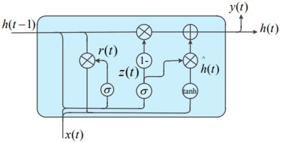
Figure 4. GRU architecture [38].

2.8. Weka and Python

The Weka software was introduced at Waikato University in New Zealand. The system was written in Java and distributed under the terms of a General Public License. Weka supports many standard data mining works such as data preprocessing, clustering, regression, classification, visualization, and feature selection. It presents a uniform interface for many different learning algorithms to evaluate the outcome of learning schemes in pre- and post- processing and in any given data set. Weka is a collection of the most advanced machine learning algorithms and data preprocessing tools [26,39].

Python is a high-level, interpreted, open-source, general-purpose programming language. Created by Guido van Rossum and released in 1991, it is used for data science, machine learning, system automation, web and API development, and more [40].

3. Results and Discussion

In this section, the results obtained according to different data mining methods and input combinations are given and compared with the deep learning technique.

The measurement of meteorological variables is difficult or costly; this was taken into account when creating scenarios. Naturally, it is desirable to estimate the amount of ETo with the help of fewer or even one or two easily measurable variables, rather than using all or multiple meteorological variables. Alternate scenarios and their input variables are given in Table 3.

Table 3. Alternative scenarios.

Scenarios	Inputs								Number of Input Parameters
	MTI	Tmin	Tmax	U2	Tdev	n	MinRH	MaxRH
1	*	*	*	*	*	*	*	*	8
2	*	*	*	*		*	*	*	7
3		*	*	*		*	*	*	6
4		*	*	*		*	*		5
5		*	*	*		*			4
6		*	*	*					3
7		*	*						2
8			*						1
9		*							1
10			*	*					2
11						*			1
12			*			*			2
13		*	*		*	*			4
14		*	*		*				3
15	*		*						2

* MTI is Monthly Time Index.

In this study, the input variables used in the formation of scenarios are based on two important factors. The first factor was based on variables affecting ETo within the framework of the theoretical approach, while the second was based on the correlation coefficient between ETo and other independent meteorological variables. The effect of a single input variable on the ETo estimation was examined in scenarios 8, 9 and 11 (Table 3).

3.1. M5P Model

The results obtained with the M5P Model are given in Table 4. As shown, the best result was obtained in the first scenario (R = 0.9925, MAE = 0.1566 mm/day, RMSE = 0.2135 mm/day), but in this scenario, there were 8 input variables. The model presented 63 different linear models for ETo calculation. In this case, the 1st scenario is quite difficult to use in terms of implementation. The 15th scenario is relatively useful when using only Tmax as a measured input (R = 0.9694, MAE = 0.319 mm/day, RMSE = 0.4277 mm/day), and is more useful than the first scenario due to the small number of parameters and the 20 linear equations it generates. According to the M5P results, even though the linear equation number is advantageous in the 6th and 10th scenarios, the accuracy rate is lower compared to the 1st and 15th scenarios, making it unsuitable for use. The results of the 1st and 15th scenarios from the M5P model are close to the results obtained from the ETo-PM model. As can be seen from Figure 5a,b, there is a high level of agreement between the values obtained from M5P and PMF-56.

Table 4. M5P model results for 15 different scenarios.

Scenarios	Evaluation Metrics					Number of Input Parameters
	R	MAE (mm/day)	RMSE (mm/day)	LM No	Run Time (s)
1	0.9925	0.1566	0.2135	63	0.18	8
2	0.9917	0.1617	0.2236	62	0.58	7
3	0.9795	0.2595	0.3506	64	0.59	6
4	0.9771	0.2745	0.3704	45	0.56	5
5	0.9692	0.3215	0.4289	45	0.56	4
6	0.9063	0.5856	0.7360	4	0.53	3
7	0.9027	0.5977	0.7493	7	0.49	2
8	0.9012	0.6013	0.7548	5	0.12	1
9	0.8742	0.6690	0.8455	5	0.13	1
10	0.9051	0.5892	0.7404	4	0.45	2
11	0.9334	0.4611	0.6250	37	0.09	1
12	0.9629	0.3509	0.4698	45	0.44	2
13	0.9763	0.2812	0.3768	21	0.55	4
14	0.9223	0.5375	0.6731	6	0.53	3
15	0.9694	0.3190	0.4277	20	0.28	2

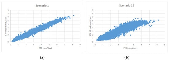
Figure 5. Scatter plot of M5P method for (a) Scenario 1 and (b) Scenario 15.

In this study, the running time of the models was affected by the processor of the used computer, the number of input variables, and the data in the scenarios. As seen in Table 4, the running time was very short. The low running time here is shown only to emphasize the advantage of the proposed method.

3.2. The Random Forest

The results of the RF model for different scenarios are provided in Table 5. As shown, the best results were obtained in the first scenario (R = 0.9926, MAE = 0.1533 mm/day, RMSE = 0.2122 mm/day), but there were 8 input variables, and it is desirable to have a small number of inputs so that the model does not become too complicated. Therefore, the use of the 1st scenario is not suitable for implementation. Scenario 15, however, when using Tmax as a measured input with a monthly time index, yielded a relatively good result (R = 0.963, MAE = 0.3486 mm/day, RMSE = 0.4697 mm/day) compared to the 1st scenario.

Table 5. RF model results for different scenarios.

Scenarios	Evaluation Metrics				Number of Input Parameters
	R	MAE (mm/day)	RMSE (mm/day)	Run Time (s)
1	0.9926	0.1533	0.2122	3.54	8
2	0.9925	0.1531	0.2136	2.60	7
3	0.9826	0.2363	0.3235	2.47	6
4	0.9799	0.2554	0.3480	3.07	5
5	0.9715	0.3045	0.4126	2.71	4
6	0.8947	0.6079	0.7789	2.07	3
7	0.8729	0.6611	0.8560	2.62	2
8	0.8971	0.6116	0.7697	0.59	1
9	0.8709	0.6753	0.8561	0.55	1
10	0.8746	0.6551	0.8507	2.63	2
11	0.9362	0.4488	0.6122	0.43	1
12	0.9586	0.3640	0.4969	2.17	2
13	0.8068	3.8546	5.1657	3.43	4
14	0.9129	0.5556	0.7113	2.37	3
15	0.963	0.3486	0.4697	1.45	2

The 1st and 15th scenario results from the RF model are very similar to the distribution of the results obtained from the ETo-PM model. As can be seen from Figure 6a,b, there is a high level of agreement between the values obtained from RF and ETo-PM. The RF model uses multiple trees because it takes variables randomly as its input, and the best model selection process is better than the M5T model because it uses the voting principle.

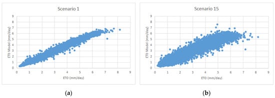
Figure 6. Scatter plot of the RF method for (a) Scenario 1 and (b) Scenario 15.

3.3. The Random Tree

As shown in Table 6, the best results were obtained in the first scenario (R = 0.9798, MAE = 0.2472 mm/day, RMSE = 0.3502 mm/day). In the 1st scenario, there were 8 input variables, but the 15th scenario yielded a result close to the 1st scenario using only Tmax as measured input with a monthly time index (R = 0.9599, MAE = 0.3591 mm/day, RMSE = 0.4895 mm/day).

Table 6. RF model results for different scenarios.

Scenarios	Evaluation Metrics				Number of Input Parameters
	R	MAE (mm/day)	RMSE (mm/day)	Run Time (s)
1	0.9798	0.2472	0.3502	0.05	8
2	0.9790	0.2502	0.3567	0.22	7
3	0.9623	0.3355	0.4768	0.03	6
4	0.9580	0.3599	0.5045	0.04	5
5	0.9459	0.4149	0.5739	0.04	4
6	0.8205	0.7909	1.0435	0.05	3
7	0.8215	0.7909	1.0368	0.03	2
8	0.8968	0.6122	0.7706	0	1
9	0.8708	0.6755	0.8563	0	1
10	0.8365	0.7485	0.9867	0.02	2
11	0.9362	0.4488	0.6120	0	1
12	0.9419	0.4285	0.5920	0.03	2
13	0.9557	0.3721	0.5168	0.05	4
14	0.8509	0.7103	0.9495	0.03	3
15	0.9599	0.3591	0.4895	0.01	2

Figure 7a,b show the results obtained from the 1st and 15th scenarios from the RT model and the distribution of the results from the ETo-PM model. As can be seen from the graphs, there was agreement between the values obtained from RT and ETo-PM.

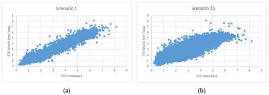
Figure 7. Scatter plot of the RF method for (a) Scenario 1 and (b) Scenario 15.

3.4. REPtree

The results of the RF model for different scenarios are given in Table 7. As shown in the table, the best results were obtained in the first scenario (R = 0.982, MAE = 0.2366 mm/day, RMSE = 0.3288 mm/day). The results of the 2nd scenario were almost the same as those of the 1st scenario. Thus, it was found that the effect of using Tdew on the model was negligible. When the 15th scenario was examined, it was seen that Reptree model gave relatively good results (R = 0.967, MAE = 0.3284 mm/day, RMSE = 0.4435 mm/day).

Table 7. REPTree model results for different scenarios.

Scenarios	Evaluation Metrics				Number of Input Parameters
	R	MAE (mm/day)	RMSE (mm/day)	Run Time (s)
1	0.9820	0.2366	0.3288	0.04	8
2	0.9820	0.2373	0.3293	0.21	7
3	0.9703	0.3052	0.4219	0.05	6
4	0.9697	0.3085	0.4256	0.03	5
5	0.9676	0.3218	0.4400	0.03	4
6	0.9000	0.5990	0.7594	0.02	3
7	0.8977	0.6079	0.7676	0.01	2
8	0.8993	0.6061	0.7615	0	1
9	0.8721	0.6729	0.8523	0	1
10	0.8972	0.6063	0.7693	0.02	2
11	0.9356	0.4514	0.6147	0	1
12	0.9620	0.3509	0.4756	0.02	2
13	0.9668	0.3273	0.4454	0.03	4
14	0.9079	0.5700	0.7313	0.03	3
15	0.9670	0.3284	0.4435	0.02	2

In Figure 8a,b, the scatter plot of the 1st and 15th scenarios of the RepTree model are given. As can be seen from the graphs, the values obtained in the RepTree method are less compatible with the M5P and RF methods.

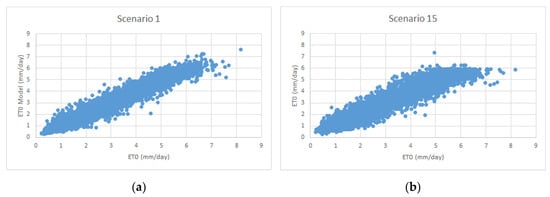
Figure 8. Scatter plot of REPTree method for (a) Scenario 1 and (b) Scenario 15.

3.5. GRU

The Python language was used to model the study with RNN-GRU. The model consists of 2 hidden layers with 200 and 150 neurons respectively. Relu was used as an activation function, and the Adam algorithm was used for optimization.

The results of the test period obtained in 15 different scenarios using the GRU model are provided in Table 8. As shown, scenario 1 using all meteorological variable as inputs gave the best result (R = 0.9931, MAE = 0.1953 mm/day, RMSE = 0.2556 mm/day). The fact that the GRU Model uses only Tmax and n as the input variable in scenario 12 is also very important for in situ applications, since the Tmax and n variables are easier and cheaper to measure. The GRU model took 204 s to complete scenario 12, as it is a deep learning mechanism and has many hidden layers. GRU trains the model more slowly than other machine learning methods, which may be a disadvantage for deep learning. However, with fast computers, it may not make sense to view this duration as a disadvantage. The 15th scenario yielded a relatively good result when only the measured Tmax variable was used with MTI (R = 0.9837, MAE = 0.2433 mm/day, RMSE = 0.3292 mm/day). For the 15th scenario, 223 s were needed. Scatter plots of scenarios 1 and 15 are presented in Figure 9a,b. As can be seen from the graphs, the results obtained from the ETo-PM method and GRU model are highly compatible.

Table 8. GRU model results for 15 different scenarios.

Scenarios	Evaluation Metrics				Number of Input Parameters
	R	MAE (mm/day)	RMSE (mm/day)	Run Time (m)
1	0.9931	0.1953	0.2556	3.15	8
2	0.9918	0.1747	0.2424	3.28	7
3	0.9747	0.3214	0.4171	3.01	6
4	0.9731	0.3304	0.4295	1.20	5
5	0.9632	0.4103	0.5252	1.42	4
6	0.9176	0.5768	0.7261	1.25	3
7	0.9131	0.5868	0.7426	2.05	2
8	0.9110	0.6193	0.7721	1.26	1
9	0.9100	0.6200	0.7661	3.22	1
10	0.9169	0.5811	0.7299	1.53	2
11	0.9851	0.2402	0.3193	1.36	1
12	0.9543	0.4481	0.5882	3.14	2
13	0.9708	0.3552	0.4719	3.24	4
14	0.9327	0.5350	0.6598	2.52	3
15	0.9837	0.2433	0.3292	3.43	2

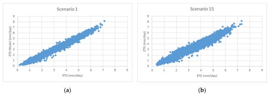
Figure 9. GRU model scatters plot for (a) scenario 1 and (b) scenario 15.

For the evaluation of overfitting/underfitting problems of the GRU model, a loss vs epoch plot is given in Figure 10. As expected, the training and test loss values are parallel and decreasing.

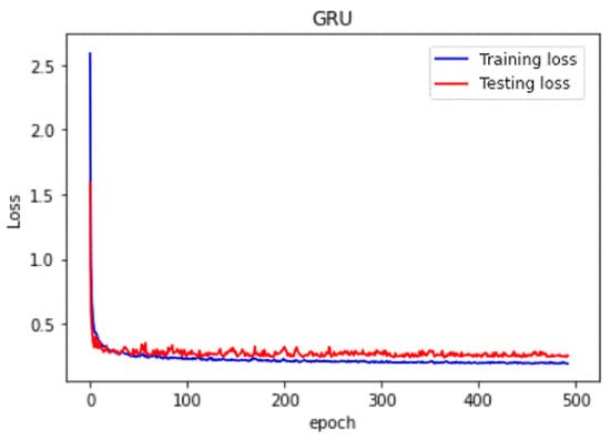
Figure 10. Loss vs epoch plot of Scenario 15 of the GRU model.

The performance of different input combinations with the models used in this study was compared according to the R values, and is summarized in Figure 11. As can be understood from the figure, scenarios with the Tmax variable as one of the meteorological parameters gave better results than the others. Scenario 1, which includes all meteorological variables, was found to be the best for all models. Among the five models used in the study, the GRU model (R = 0.9931) based on the deep learning mechanism, gave the best result.

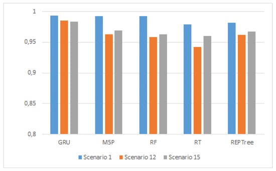
Figure 11. Comparison of R values of models according to scenarios.

The statistical properties of the ETo values obtained from different models and ETo-PM are given in Table 9. As shown, the statistical properties of the methods used were quite similar to the those of the ETo-PM method, except for the GRU model. The GRU results showed less similarity than other methods. In this respect, the GRU results showed less success than the other methods, especially compared to standard deviation values.

Table 9. Comparison of ETo statistical features based on used models.

Method	Scenario	Minimum	Maximum	Mean	Std. Deviation
M5P	1	0.174	7.556	2.686	1.726
	15	0.510	6.701	2.689	1.685
RF	1	0.316	6.855	2.687	1.709
	15	0.272	7.579	2.688	1.699
RF	1	0.291	8.169	2.690	1.740
	15	0.223	8.169	2.688	1.705
REP Tree	1	0.292	7.616	2.690	1.718
	15	0.291	7.320	2.688	1.691
GRU	1	0.190	7.128	2.685	1.623
	15	0.382	7.319	2.679	1.687
ETo-PM (mm/day)		0.223	8.169	2.687	1.742

In this study, to better evaluate the performance of the models used, a Taylor diagram was drawn according for scenarios 1 and 15 (Figure 12). As can be seen from Figure 11, the M5P method yielded results that were closer to observed values than those of the other methods for scenario 1. M5P is followed by RF and GRU. As can be seen from this graph, the results of the RT and REPTree models were located at a greater distance from the observed values in terms of the correlation coefficient, and thus, seemed to be relatively unsuccessful compared to other models. The Taylor diagram of the 15th scenario shows that the GRU model was closest to the ETo-PM. Another visual result of the Taylor diagram of the 15th scenario is that the other four models were located close to each other.

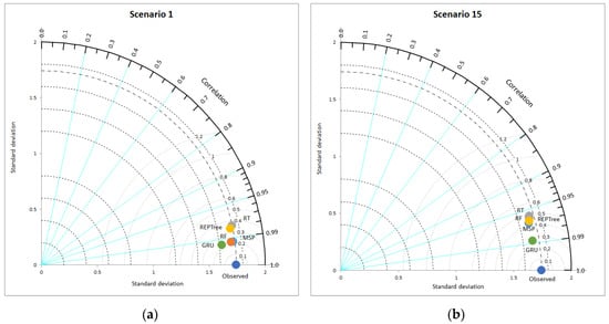
Figure 12. Taylor diagrams for ETo estimations based on used models (a) Scenario 1 and (b) Scenario 15.

In this study, as in similar studies, the amount of ETo was estimated by some artificial intelligence methods. The accuracy rate obtained in this study was similar to those of previous studies [8,9,10,14,15], i.e., in the range of R = 0.8 to 0.99. It showed that artificial intelligence models were successful in ETo predictions. The most important contribution of this study, compared to other studies [5,6,7,11,23], is that deep learning techniques were tested for the first time using data from Turkey’s coast; they showed good success rates with input parameters based only on temperature.

4. Conclusions

Accurate estimations of ETo quantities are essential for the efficient use of water for irrigation in agricultural economies. ETo calculations can be made with many nonlinear and multiparameter experimental equations. These experimental equations are really difficult and time consuming to use. However, it was observed that various phenomena with nonlinear structures were calculated with data-based and machine learning methods without much difficulty. The evapotranspiration phenomenon contains a complex and nonlinear structure as an important element of the hydrology cycle. In this study, the feasibility of different data mining methods and deep learning models on ETo estimation were evaluated. According to the obtained results, when considering different combinations of meteorological variables as inputs, the RF and GRU methods achieved high levels of success in ETo estimations compared to other methods. In this study, as a result of comparing different input scenarios, it was seen that the maximum temperature parameter is the most important input variable for ETo prediction models. This indicates that temperature is an important variable in ETo formation, since the region is humid. The measurement of temperature is very easy, simple, and cost-effective compared to other meteorological variables. The results of this study were analyzed; it can be seen that the findings were very close to those of previous studies [14,15]. As a result, given the limited meteorological data in humid areas, a high level of accuracy and easy predictability of the ETo amount were achieved using only the maximum temperature data. The most important contributions of this study are (1) its evaluation of the performance of the GRUs method, which is a deep learning method, with an estimate of ETo, and (2) its very successful ETo predictions with only one meteorological variable. It is recommended that the proposed method be used to calculate ETo without the need of other meteorological parameters.

References

- Unlukara, A.; Kurunc, A.; Cemek, B. Green Long Pepper Growth under Different Saline and Water Regime Conditions and Usability of Water Consumption in Plant Salt Tolerance. J. Agric. Sci. 2015, 21, 167–176. [Google Scholar]
- Bruin, H.; Trigo, I. A New Method to Estimate Reference Crop Evapotranspiration from Geostationary Satellite Imagery: Practical Considerations. Water 2019, 11, 382. [Google Scholar] [CrossRef]
- Hamoud, A.; Hashim, A.S.; Awadh, W.A. Predicting Student Performance in Higher Education Institutions Using Decision Tree Analysis. Int. J. Interact. Multimed. Artif. Intell. 2018, 5, 26. [Google Scholar] [CrossRef]
- Romero, Á.; Dorronsoro, J.R.; Díaz, J. Day-Ahead Price Forecasting for the Spanish Electricity Market. Int. J. Interact. Multimed. Artif. Intell. 2019, 5, 42. [Google Scholar] [CrossRef]
- Pal, M.; Deswal, S. M5 model tree based modelling of reference evapotranspiration. Hydrol. Process. 2009, 23, 1437–1443. [Google Scholar] [CrossRef]
- Sattari, M.T.; Pal, M.; Yurekli, K.; Unlukara, A. M5 model trees and neural network based modelling of ET0 in Ankara, Turkey. Turk. J. Eng. Environ. Sci. 2013, 37, 211–220. [Google Scholar] [CrossRef][Green Version]
- Esmaeilzadeh, B.; Sattari, M.T. Monthly evapotranspiration modeling using intelligent systems in Tabriz, Iran. Agric. Sci. Dev. 2015, 4, 35–40. [Google Scholar]
- Rahimikhoob, A. Comparison of M5 Model Tree and Artificial Neural Network’s Methodologies in Modelling Daily Reference Evapotranspiration from NOAA Satellite Images. Water Resour. Manag. 2016, 30, 3063–3075. [Google Scholar] [CrossRef]
- Feng, Y.; Cui, N.; Gong, D.; Zhang, Q.; Zhao, L. Evaluation of random forests and generalized regression neural networks for daily reference evapotranspiration modelling. Agric. Water Manag. 2017, 193, 163–173. [Google Scholar] [CrossRef]
- Shiri, J. Improving the performance of the mass transfer-based reference evapotranspiration estimation approaches through a coupled wavelet-random forest methodology. J. Hydrol. 2018, 561, 737–750. [Google Scholar] [CrossRef]
- Fan, J.; Yue, W.; Wu, L.; Zhang, F.; Cai, H.; Wang, X.; Lu, X.; Xiang, Y. Evaluation of SVM, ELM and four tree-based ensemble models for predicting daily reference evapotranspiration using limited meteorological data in different climates of China. Agric. For. Meteorol. 2018, 263, 225–241. [Google Scholar] [CrossRef]
- Guo, H.; Zhuang, X.; Rabczuk, T. A Deep Collocation Method for the Bending Analysis of Kirchhoff Plate. Comput. Mater. Contin. 2019, 59, 433–456. [Google Scholar] [CrossRef]
- Anitescu, C.; Atroshchenko, E.; Alajlan, N.; Rabczuk, T. Artificial Neural Network Methods for the Solution of Second Order Boundary Value Problems. Comput. Mater. Contin. 2019, 59, 345–359. [Google Scholar] [CrossRef]
- Granata, F. Evapotranspiration evaluation models based on machine learning algorithms—A comparative study. Agric. Water Manag. 2019, 217, 303–315. [Google Scholar] [CrossRef]
- Wang, S.; Lian, J.; Peng, Y.; Hu, B.; Chen, H. Generalized reference evapotranspiration models with limited climatic data based on random forest and gene expression programming in Guangxi, China. Agric. Water Manag. 2019, 221, 220–230. [Google Scholar] [CrossRef]
- Chia, M.Y.; Huang, Y.F.; Koo, C.H.; Fung, K.F. Recent Advances in Evapotranspiration Estimation Using Artificial Intelligence Approaches with a Focus on Hybridization Techniques—A Review. Agronomy 2020, 10, 101. [Google Scholar] [CrossRef]
- Srivastava, P.K.; Singh, P.; Mall, R.K.; Pradhan, R.K.; Bray, M.; Gupta, A. Performance assessment of evapotranspiration estimated from different data sources over agricultural landscape in Northern India. Theor. Appl. Clim. 2020. [Google Scholar] [CrossRef]
- Anonymous. Tekirdag Investment Environment; Tekirdag Development Agency: Tekirdağ, Turkey, 2014. [Google Scholar]
- Anonymous. Tekirdag Province Agricultural Investment Guide; Ministry of Food, Agriculture and Livestock, Strategy Development: Tekirdağ, Turkey, 2018. [Google Scholar]
- Corine Landuse for Turkey. Available online: https://corinecbs.tarimorman.gov.tr (accessed on 1 March 2020).
- Doorenbos, J.; Pruitt, W.O. Crop Water Requirements; FAO Irrigation and Drainage Paper 24; FAO: Rome, Italy, 1977; p. 144. [Google Scholar]
- Allen, R.G.; Pereira, L.S.; Raes, D.; Smith, M. Crop Evapotranspiration—Guidelines for Computing Crop Water Requirements—FAO Irrigation and Drainage Paper 56; FAO: Rome, Italy, 1998; ISBN 92-5-104219-5. [Google Scholar]
- Gavili, S.; Sanikhani, H.; Kisi, O.; Mahmoudi, M.H. Evaluation of several soft computing methods in monthly evapotranspiration modelling. Meteorol. Appl. 2017, 25, 128–138. [Google Scholar] [CrossRef]
- Timofeev, R. Classification and Regression Trees (CART) Theory and Applications. Master’s Thesis, Humboldt University, Berlin, Germany, 2004. [Google Scholar]
- Sullivan, W. Decision Tree and Random Forest—Machine Learning and Algorithms; CreateSpace Publishing: Scotts Valley, CA, USA, 2018; ISBN 1986246663, 9781986246668. [Google Scholar]
- Witten, I.H.; Frank, E. Data Mining: Practical Machine Learning Tools and Techniques, 2nd ed.; Morgan Kaufmann Series in Data Management Systems: Washington, DC, USA, 2005. [Google Scholar]
- Quinlan, J. Simplifying decision trees. Int. J. Man-Mach. Stud. 1987, 27, 221–234. [Google Scholar] [CrossRef]
- Cutler, A.; Cutler, D.R.; Stevens, J.R. Random Forests. In Ensemble Machine Learning; Zhang, C., Ma, Y., Eds.; Springer: Boston, MA, USA, 2012. [Google Scholar]
- Pfahringer, B. Random Model Trees: An Effective and Scalable Regression Method University of Waikato, New Zealand. 2019. Available online: http://www.cs.waikato.ac.nz/~bernhard (accessed on 1 March 2020).
- García-Peñalvo, F.; Cruz-Benito, J.; Martin-Gonzalez, M.; Vázquez-Ingelmo, A.; Sánchez-Prieto, J.C.; Therón, R. Proposing a Machine Learning Approach to Analyze and Predict Employment and its Factors. Int. J. Interact. Multimed. Artif. Intell. 2018, 5, 39. [Google Scholar] [CrossRef]
- Breiman, L. Random Forests. Mach. Learn. 2001, 45, 5–36. [Google Scholar] [CrossRef]
- Sheppard, C. Tree-Based Machine Learning Algorithms: Decision Trees, Random Forests, and Boosting; CreateSpace Publishing: Scotts Valley, CA, USA, 2017; ISBN 1975860977, 9781975860974. [Google Scholar]
- Akman, M.; Genc, Y.; Ankarali, H. Random forests methods and practices in a health field. Turk. Clin. J. Biostat. 2011, 3, 36–48. (In Turkish) [Google Scholar]
- Suchetana, B.; Rajagopalan, B.; Silverstein, J. Assessment of wastewater treatment facility compliance with decreasing ammonia discharge limits using a regression tree model. Sci. Total. Environ. 2017, 598, 249–257. [Google Scholar] [CrossRef] [PubMed]
- Watts, J.D.; Powell, S.L.; Lawrence, R.; Hilker, T. Improved classification of conservation tillage adoption using high temporal and synthetic satellite imagery. Remote Sens. Environ. 2011, 115, 66–75. [Google Scholar] [CrossRef]
- Cho, K.; Van Merrienboer, B.; Gulcehre, C.; Bahdanau, D.; Bougares, F.; Schwenk, H.; Bengio, Y. Learning Phrase Representations using RNN Encoder-Decoder for Statistical Machine Translation. In Proceedings of the 2014 Conference on Empirical Methods in Natural Language Processing (EMNLP), Doha, Qatar, 25–29 October 2014. [Google Scholar]
- Chung, J.; Gulcehre, C.; Cho, K.; Bengio, Y. Empirical Evaluation of Gated Recurrent Neural Networks on Sequence Modeling. arXiv 2014, arXiv:1412.3555. [Google Scholar]
- Wang, Y.; Liao, W.; Chang, Y. Gated Recurrent Unit Network-Based Short-Term Photovoltaic Forecasting. Energies 2018, 11, 2163. [Google Scholar] [CrossRef]
- Witten Ian, H.; Eibe, F.; Hall Mark, A. Data Mining Practical Machine Learning Tools and Techniques, 3rd ed.; Morgan Kaufmann Publishers is an Imprint of Elsevier: Amsterdam, The Netherlands, 2011. [Google Scholar]
- Kuhlman, D. A Python Book: Beginning Python, Advanced Python, and Python Exercises; Platypus Global Media: Warsaw, Poland, 2013. [Google Scholar]
© 2020 by the authors. Licensee MDPI, Basel, Switzerland. This article is an open access article distributed under the terms and conditions of the Creative Commons Attribution (CC BY) license (http://creativecommons.org/licenses/by/4.0/).