Article

Mean Shift versus Variance Inflation Approach for Outlier Detection—A Comparative Study

1
Faculty of Spatial Information, University of Applied Sciences Dresden, 01069 Dresden, Germany
2
Faculty 1: Architecture—Civil Engineering—Geomatics, Frankfurt University of Applied Sciences, 60318 Frankfurt, Germany
3
Technische Universität Berlin, Institute of Geodesy and Geoinformation Science, 10623 Berlin, Germany
*
Author to whom correspondence should be addressed.
Mathematics 2020, 8(6), 991; https://doi.org/10.3390/math8060991
Submission received: 8 May 2020 / Revised: 10 June 2020 / Accepted: 12 June 2020 / Published: 17 June 2020
(This article belongs to the Special Issue Stochastic Models for Geodesy and Geoinformation Science)

Abstract

:
Outlier detection is one of the most important tasks in the analysis of measured quantities to ensure reliable results. In recent years, a variety of multi-sensor platforms has become available, which allow autonomous and continuous acquisition of large quantities of heterogeneous observations. Because the probability that such data sets contain outliers increases with the quantity of measured values, powerful methods are required to identify contaminated observations. In geodesy, the mean shift model (MS) is one of the most commonly used approaches for outlier detection. In addition to the MS model, there is an alternative approach with the model of variance inflation (VI). In this investigation the VI approach is derived in detail, truly maximizing the likelihood functions and examined for outlier detection of one or multiple outliers. In general, the variance inflation approach is non-linear, even if the null model is linear. Thus, an analytical solution does usually not exist, except in the case of repeated measurements. The test statistic is derived from the likelihood ratio (LR) of the models. The VI approach is compared with the MS model in terms of statistical power, identifiability of actual outliers, and numerical effort. The main purpose of this paper is to examine the performance of both approaches in order to derive recommendations for the practical application of outlier detection.

1. Introduction

Nowadays, outlier detection in geodetic observations is part of the daily business of modern geodesists. As Rofatto et al. [1] state, we have well established and practicable methods for outlier detection for half a century, which are also implemented in current standard geodetic software. The most important toolbox for outlier detection is the so-called data snooping, which is based on the pioneering work of Baarda [2]. A complete distribution theory of data snooping, also known as DIA (detection, identification, and adaptation) method, was developed by Teunissen [3].
In geodesy, methods for outlier detection can be characterised as statistical model selection problem. A null model is opposed to one or more extended or alternative models. While the null model describes the expected stochastic properties of the data, the alternative models deviate from such a situation in one way or another. For outlier detection, the alternative models relate to the situation, where the data are contaminated by one or more outliers. According to Lehmann [4], an outlier is defined by “an observation that is so probably caused by a gross error that it is better not used or not used as it is”.
From a statistical point of view, outliers can be interpreted as a small amount of data that have different stochastic properties than the rest of the data, usually a shift in the mean or an inflation of the variance of their statistical distribution. This situation is described by extra parameters in the functional or stochastic model, such as shifted means or inflated variances. Such an extended model is called an alternative model. Due to the additionally introduced parameters, the discrepancies between the observations and the related results of the model decrease w. r. t. the null model. It has to be decided whether such an improvement of the goodness of fit is statistically significant, which means that the alternative model describes the data better than the null model. This decision can be made by hypothesis testing, information criteria, or many other statistical decision approaches, as shown by Lehmann and Lösler [5,6].
The standard alternative model in geodesy is the mean shift (MS) model, in which the contamination of the observations by gross errors is modelled as a shift in the mean, i.e., by a systematic effect. This approach is described in a large number of articles and textbooks, for example, the contributions by Baarda [2], Teunissen [7], and Kargoll [8]. However, there are other options besides this standard procedure. The contamination may also be modelled as an inflation of the variance of the observations under consideration, i.e., by a random effect. This variance inflation (VI) model is rarely investigated in mathematical statistics or geodesy. Bhar and Gupta [9] propose a solution based on Cook’s statistic [10]. Although this statistic was invented for the MS model, it can also be made applicable when the variance is inflated.
Thompson [11] uses the VI model for a single outlier in the framework of the restricted (or residual) maximum likelihood estimation, which is known as REML. In contrast to the true maximum likelihood estimation, REML can produce unbiased estimates of variance and covariance parameters and it causes less computational workload. Thompson [11] proposes that the observation with the largest log-likelihood value can be investigated as a possible outlier. Gumedze et al. [12] take up this development and set up a so-called variance shift outlier model (VSOM). Likelihood ratio (LR) and score test statistics are used to identify the outliers. The authors conclude that VSOM gives an objective compromise between including and omitting an observation, where its status as a correct or erroneous observation cannot be adequately resolved. Gumedze [13] review this approach and work out a one-step LR test, which is a computational simplification of the full-step LR test.
In geodesy, the VI model was introduced by Koch and Kargoll [14]. The estimation of the unknown parameters has been established as an iteratively reweighted least squares adjustment. The expectation maximization (EM) algorithm is used to detect the outliers. It is found that the EM algorithm for the VI model is very sensitive to outliers, due to its adaptive estimation, whereas the EM algorithm for the MS model provides the distinction between outliers and good observations. Koch [15] applies the method to fit a surface in three-dimensional space to the Cartesian coordinates of a point cloud obtained from measurements with a laser scanner.
The main goal of this contribution is a detailed derivation of the VI approach in the framework of outlier detection and compare it with the well-established MS model. The performance of both approaches is to be compared in order to derive recommendations for the practical application of outlier detection. This comprises the following objectives:
  • Definition of the generally accepted null model and specification of alternative MS and VI models (Section 2). Multiple outliers are allowed for in both alternative models to keep the models equivalent.
  • True maximization of the likelihood functions of the null and alternative models, not only for the common MS model, but also for the VI model. This means, we do not resort to the REML approach of Thompson [11], Gumedze et al. [12], and Gumedze [13]. This is important for the purpose of an insightful comparison of MS and VI (Section 3).
  • Application of likelihood ratio (LR) test for outlier detection by hypothesis testing and derivation of the test statistics for both the MS and the VI model. For this purpose, a completely new rigorous likelihood ratio test in the VI model is developed and an also completely new comparison with the equivalent test in the MS model is elaborated (Section 3).
  • Comparison of both approaches using the illustrative example of repeated observations, which is worked out in full detail (Section 4).
Section 5 briefly summarises the investigations that were carried out and critically reviews the results. Recommendations for the practical application of outlier detection conclude this paper.

2. Null Model, Mean Shift Model, and Variance Inflation Model

In mathematical statistics, a hypothesis H is a proposed explanation that the probability distribution of the random n-vector y of observations belongs to a certain parametric family W of probability distributions with parameter vector θ , e.g., Teunissen [7],
H : y W ( θ ) , θ Θ
The parameter vector θ might assume values from a set Θ of admissible parameter vectors. A model is then simply the formulation of the relationship between observations y and parameters θ based on H. In geodesy, the standard linear model is based on the hypothesis that the observations follow a normal distribution N, e.g., Koch [16], Teunissen [7], i.e.,
H 0 : y N ( A x , Σ ) ,
with u-vector of functional parameters x and covariance matrix Σ . The latter matrix might contain further stochastic parameters, like a variance factor σ 2 , according to
Σ = σ 2 Q ,
with Q being the known cofactor matrix of y. In this case, θ is the union of x and σ 2 . The covariance matrix Σ might eventually contain more stochastic parameters, known as variance components, cf. Koch ([16], p. 225ff). Matrix A is said to be the n × u -matrix of design. The model that is based on H 0 is called the null model.
In outlier detection, we oppose H 0 with one or many alternative hypotheses, most often in the form of a mean shift (MS) hypothesis, e.g., Koch [16], Teunissen [7]
H M S : y N ( A x + C , Σ ) , 0 ,
where ∇ is a m-vector of additional functional bias parameters and matrix C extends the design. In this case, θ is extended by ∇. This relationship gives rise to the MS model, where the mean of the observations is shifted from A x to A x + C by the effect of gross errors, see Figure 1. C can be interpreted as accounting for the systematic effect of gross observation errors superposing the effect of normal random observation errors already taken into account by Σ in (2). The great advantage of H M S is that, if the null model is linear or linearized, so is the MS model. The determination of the model parameters is numerically easy and computationally efficient, cf. Lehmann and Lösler [5].
However, there are different possibilities to set up an alternative hypothesis. The most simple one is the variance inflation hypothesis
H V I : y N ( A x , Σ ) ,
where Σ is a different covariance matrix, which consists of inflated variances. Σ can be interpreted as accounting for the joint random effect of normal observation errors in all observations and zero mean gross errors in few outlying observations, see Figure 2.
The VI model might be considered to be more adequate to describe the outlier situation when the act of falsification of the outlying observations is thought of as being a random event, which might not be exactly reproduced in a virtual repetition of the observations. However, even if the VI model might be more adequate to describe the stochastics of the observations, this does not mean that it is possible to estimate parameters or to detect outliers better than with some less adequate model like MS. This point will be investigated below.
In the following we will only consider the case that y are uncorrelated observations, where both Σ and Σ are diagonal matrices, such that the hypotheses read
H 0 : y N ( A x , σ 1 2 , , σ n 2 ) ,
H V I : y N ( A x , τ 1 σ 1 2 , , τ m σ m 2 , σ m + 1 2 , , σ n 2 ) , τ 1 > 1 , , τ m > 1 .
Here, H V I accounts for m random zero mean gross errors in the observations y 1 , , y m modeled by stochastic parameters τ 1 , , τ m . In this case, θ is extended by τ 1 , , τ m , which will be called variance inflation factors. Thus, τ 1 , , τ m can be interpreted as a special case of extra variance components.
Note that the term variance inflation factors is used differently in multiple linear regression when dealing with multicollinearity, cf. James et al. ([17], p. 101f).

3. Outlier Detection by Hypothesis Tests

Outlier detection can be characterised as a statistical model selection problem. The null model, which describes the expected stochastic properties of the data, is opposed to one or more alternative models, which deviate from such properties. Usually, the decision, whether the null model is rejected in favour of a proper alternative model, is based on hypothesis testing. Multiple testing, consisting of a sequence of testings with one single alternative hypothesis only, is required if there are many possible alternative models. In this study, we first focus on such one single testing only. In the following subsections, the test statistics in the MS model as well as in the VI model are derived.
For the sake of simplicity, the scope of this contribution is restricted to cases, where all of the estimates to be computed are unique, such that all matrices to be inverted are regular.

3.1. Mean Shift Model

In the case of no stochastic parameters, i.e., Σ is known, the optimal test statistic T M S ( y ) for the test problem H 0 in (2) versus H M S in (4) is well known and yields, cf. Teunissen ([7], p. 76):
T M S ( y ) : = ^ T Σ ^ 1 ^ = e ^ 0 T Σ 1 C ( C T Σ 1 Σ e ^ 0 1 Σ 1 ) 1 C T Σ 1 e ^ 0 ,
where ^ and Σ ^ are the vector of estimated bias parameters in the MS model and its covariance matrix, respectively. Furthermore, e ^ 0 and Σ e ^ 0 are the vector of estimated residuals e : = A x y in the null model and its covariance matrix, respectively. This second expression offers the opportunity to perform the test purely based on the estimation in the null model, cf. Teunissen ([7], p. 75), i.e.,
x ^ 0 = ( A T Σ 1 A ) 1 A T Σ 1 y ,
e ^ 0 = ( I A ( A T Σ 1 A ) 1 A T Σ 1 ) y ,
Σ e ^ 0 = Σ A ( A T Σ 1 A ) 1 A T .
Each estimation is such that the likelihood function of the model is maximized. The hat will indicate maximum likelihood estimates below.
The test statistic (7) follows the central or non-central χ 2 distributions
T M S | H 0 χ 2 ( q , 0 ) ,
T M S | H M S χ 2 ( q , λ ) ,
where q = rank ( Σ ^ ) is the degree of freedom and λ = T Σ ^ 1 is called the non-centrality parameter, depending on the true but unknown bias parameters ∇, e.g., (Teunissen [7], p. 77).
The test statistic (7) has the remarkable property of being uniformly the most powerful invariant (UMPI). This means, given a probability of type 1 decision error (rejection of H 0 when it is true) α , (7)
  • has the least probability of type 2 decision error (failure to reject H 0 when it is false) β (most powerful);
  • is independent of ∇ (uniform); and,
  • but only for some transformed test problem (invariant).
For the original test problem, no uniformly most powerful (UMP) test exists. For more details see Arnold [18], Kargoll [8].
Lehmann and Voß-Böhme [19] prove that (7) has the property of being a UMP χ 2 test, i.e., a UMP test in the class of all tests with test statistic following a χ 2 distribution. It can be shown that (7) belongs to the class of likelihood ratio (LR) tests, where the test statistic is equivalent to the ratio
max L 0 ( x ) max L M S ( x , ) .
Here, L 0 and L M S denote the likelihood functions of the null and alternative model, respectively, cf. Teunissen ([7], p. 53), Kargoll [8]. (Two test statistics are said to be equivalent, if they always define the same critical region and, therefore, bring about the same decision. A sufficient condition is that one test statistic is a monotone function of the other. In this case, either both or none exceed their critical value referring to the same α .) The LR test is very common in statistics for the definition of a test statistic, because only a few very simple test problems permit the construction of a UMP test. A justification for this definition is provided by the famous Neyman-Pearson lemma, cf. Neyman and Pearson [20].

3.2. Variance Inflation Model

For the test problem (6a) versus (6b), no UMP test exists. Therefore, we also resort to the LR test here. We start by setting up the likelihood functions of the null and alternative model. For the null model (6a), the likelihood function reads
L 0 ( x ) = ( 2 π ) n 2 i = 1 n σ i 1 exp Ω 0 2 ,
Ω 0 : = i = 1 n ( y i a i x ) 2 σ i 2 ,
and for the alternative model (6b) the likelihood function is given by
L V I ( x , τ 1 , , τ m ) = ( 2 π ) n 2 i = 1 n σ i 1 i = 1 m τ i 1 2 exp Ω V I 2 ,
Ω V I : = i = 1 m ( y i a i x ) 2 σ i 2 τ i + i = m + 1 n ( y i a i x ) 2 σ i 2 ,
where a i , i = 1 , , n are the row vectors of A. According to (10), the likelihood ratio reads
max L 0 ( x ) max L V I ( x , τ 1 , , τ m ) = max exp Ω 0 2 max i = 1 m τ i 1 2 exp Ω V I 2 .
Equivalently, we might use the double negative logarithm of the likelihood ratio as test statistic, because it brings about the same decision as the likelihood ratio itself, i.e.,
T V I : = 2 log max exp Ω 0 2 max i = 1 m τ i 1 2 exp Ω V I 2 = min Ω 0 min Ω V I + i = 1 m log τ i .
The first minimization result is the well-known least squares solution (8). The second minimization must be performed not only with respect to x, but also with respect to the unknown variance inflation factors τ 1 , , τ m . The latter yield the necessary conditions
τ ^ i = ( y i a i x ^ V I ) 2 σ i 2 = e ^ V I , i 2 σ i 2 , i = 1 , , m .
This means that τ 1 , , τ m are estimated, such that the first m residuals in the VI model e ^ V I , i equal in magnitude their inflated standard deviations σ i τ ^ i , and the subtrahend in (14) is obtained by
min Ω V I + i = 1 m log τ i = min m + i = 1 m log ( y i a i x V I ) 2 σ i 2 + i = m + 1 n ( y i a i x V I ) 2 σ i 2 = min m + i = 1 m log e V I , i 2 σ i 2 + i = m + 1 n e V I , i 2 σ i 2 .
In the latter expression the minimum is to be found only with respect to the free parameter vector x V I . This expression differs from min Ω 0 essentially by the logarithm of the first m normalized residuals. This means that those summands are down-weighted, whenever the residuals e ^ V I , i are larger in magnitude than their non-inflated standard deviations σ i . The necessary conditions for x V I are obtained by nullifying the first derivatives of (16) and read
0 = i = 1 m a i j y i a i x ^ V I + i = m + 1 n y i a i x ^ V I σ i 2 a i j , j = 1 , , u ,
where a i j denotes the j-th element of a i .
This system of equations can be rewritten as a system of polynomials of degree m + 1 in the parameters x ^ V I , i . In general, the solution for x ^ V I must be executed by a numerical procedure. This extra effort is certainly a disadvantage of the VI model.
Another disadvantage is that (14) does not follow a well known probability distribution, which complicates the computation of the critical value, being the quantile of this distribution. Such a computation is best performed by Monte Carlo integration, according to Lehmann [21].
Note that the likelihood function L V I in (12) has poles at τ i = 0 , i = 1 , , m . These solutions must be excluded from consideration, because they belong to minima of (12) or equivalently to maxima of (16). (Note that log τ i is dominated by 1 / τ i at τ i 0 ).
A special issue in the VI model is what to do if max τ i ^ 1 is found in (15). In this case, the variance is not inflated, such that H 0 must not be rejected in favour of H V I , see (6b). However, it might happen that, nonetheless, T V I in (14) exceeds its critical value, especially if α is large. In order to prevent this behaviour, we modify (14) by
T V I ( y ) : = 0 if max τ i ^ 1 , min Ω 0 min Ω V I + i = 1 m log τ i otherwise .
If H 0 is true, then there is a small probability that max τ i ^ > 1 and, consequently, T V I > 0 arises, i.e.,
Pr ( T V I > 0 | H 0 ) = : α max .
We see that a type 1 error cannot be required more probable than this α max , i.e., contrary to the MS model, there is an upper limit for the choice of α .
Even more a problem is what to do, if min τ i ^ < 1 < max τ i ^ is found in (15). Our argument is that, in this case, H 0 should be rejected, but possibly not in favour of H V I in (6b). A more suitable alternative hypothesis should be found in the framework of a multiple test.

4. Repeated Observations

There is one case, which permits an analytical treatment, even of the VI model, i.e., when one scalar parameter x is observed directly n times, such that we obtain A = ( 1 , , 1 ) T = : 1 . By transformation of the observations, also all other models with u = 1 can be mapped to this case. For compact notation, we define the weighted means of all observations and of only the last n m inlying observations, i.e.,
w : = i = 1 n y i σ i 2 i = 1 n σ i 2 ,
W : = i = m + 1 n y i σ i 2 i = m + 1 n σ i 2 .
By covariance propagation, the related variances of those expressions are obtained, i.e.,
σ w 2 = 1 i = 1 n σ i 2 ,
σ W 2 = 1 i = m + 1 n σ i 2 .
Having the following useful identities
w σ w 2 = W σ W 2 + i = 1 m y i σ i 2 ,
1 σ w 2 = 1 σ W 2 + i = 1 m 1 σ i 2 , w W = σ w 2 W σ W 2 W σ w 2 + σ w 2 i = 1 m y i σ i 2
= σ w 2 i = 1 m y i W σ i 2 ,
the estimates in the null model (8) can be expressed as
x ^ 0 = w ,
e ^ 0 = y 1 w ,
Σ e ^ 0 = Σ 1 1 T σ w 2 ,
and the minimum of the sum of the squared residuals is
min Ω 0 = i = 1 n ( y i w ) 2 σ i 2 .

4.1. Mean Shift Model

In the MS model, the first m observations are falsified by bias parameters 1 , , m . Matrix
C = I 0
in (4) is a block matrix of the m × m identity matrix and a ( n m ) × m null matrix. Maximizing the likelihood function yields the estimated parameters and residuals, i.e.,
x ^ M S = W ,
e ^ M S = y 1 W ,
respectively, as well as the estimated bias parameters and their related covariance matrix, i.e.,
^ = y 1 W y m W = e ^ M S , 1 e ^ M S , m ,
Σ ^ = σ 1 2 + σ W 2 σ W 2 σ W 2 σ W 2 σ 2 2 + σ W 2 σ W 2 σ W 2 σ W 2 σ m 2 + σ W 2 ,
respectively. Note that (25d) is obtained by covariance propagation that was applied to (25c). By applying the Sherman–-Morrison formula, cf. Sherman and Morrison [22], the inverse matrix of Σ ^ is obtained,
Σ ^ 1 = σ 1 2 0 0 0 σ 2 2 0 0 0 σ m 2 + σ W 2 1 1 T 1 = σ 1 2 0 0 0 σ 2 2 0 0 0 σ m 2 σ W 2 1 + σ W 2 i = 1 m σ i 2 σ 1 2 σ 2 2 σ m 2 σ 1 2 σ 2 2 σ m 2 T = σ 1 2 0 0 0 σ 2 2 0 0 0 σ m 2 σ w 2 σ 1 4 σ 1 2 σ 2 2 σ 1 2 σ m 2 σ 1 2 σ 2 2 σ 2 4 σ 2 2 σ m 2 σ 1 2 σ m 2 σ 2 2 σ m 2 σ m 4 ,
and the test statistic (7) in the MS model becomes
T M S ( y ) = i = 1 m e ^ M S , i 2 σ i 2 σ w 2 i = 1 m j = 1 m e ^ M S , i e ^ M S , j σ i 2 σ j 2 .
According to (9), the distributions of the null model and the alternative model are given by
T M S | H 0 χ 2 ( m , 0 ) ,
T M S | H M S χ 2 ( m , λ ) ,
respectively, where the non-centrality parameter reads
λ = i = 1 m i 2 σ i 2 σ w 2 i = 1 m j = 1 m i j σ i 2 σ j 2 .
For the special cases of m = 1 and m = 2 extra bias parameters, as well as the case of independent and identically distributed random observation errors, the related test statistics (27) are given by
Case m = 1 :
T M S ( y ) = e ^ M S , 1 2 σ 1 2 + σ W 2 ,
Case m = 2 :
T M S ( y ) = e ^ M S , 1 2 σ 1 2 σ w 2 σ 1 4 + e ^ M S , 2 2 σ 2 2 σ w 2 σ 2 4 2 σ w 2 e ^ M S , 1 e ^ M S , 2 σ 1 2 σ 2 2 ,
Case σ 1 = σ 2 = = σ m = : σ :
T M S ( y ) = 1 σ 2 i = 1 m e ^ M S , i 2 1 n i = 1 m j = 1 m e ^ M S , i e ^ M S , j .
In the case of σ w min σ i , which often arises when m n , the test statistic tends to
T M S ( y ) i = 1 m e ^ M S , i 2 σ i 2 .

4.2. Variance Inflation Model—General Considerations

In the VI model, the first m observations are falsified by variance inflation factors τ 1 , , τ m . The necessary condition (17) reads
0 = i = 1 m 1 y i x ^ V I + i = m + 1 n y i x ^ V I σ i 2 .
Using (20b) and (21b), this can be rewritten to
x ^ V I W = i = 1 m σ W 2 y i x ^ V I .
This solution x ^ V I is obtained as the real root of a polynomial of degree m + 1 , which might have, at most m + 1 , real solutions. In the model, it is easy to exclude the case that y i = y j , i j , because they are either both outliers or both good observations. They should be merged into one observation. Let us index the observations, as follows: y 1 < y 2 < < y m . We see that
  • in the interval y 1 of x ^ V I the right hand side of (35) goes from 0 to + ,
  • in each interval y i 1 y i it goes from to + , and
  • in the interval y m + it goes from to 0.
  • The left hand side of (35) is a straight line.
Therefore, (35) has always at least one real solution x ^ V I in each interval y i 1 y i , where one of them must be a maximum of (16), because (16) goes from up to some maximum and then down again to in this interval. Besides these m 1 uninteresting solutions, (35) can have no more or two more real solutions, except in rare cases, where it might have one more real solution. If W < y 1 , then there are no solutions above y m . If W > y m , then there are no solutions below y 1 .
From these considerations it becomes clear that (35) can have, at most, one solution that is a minimum of (16), see also Figure 3.
The second-order sufficient condition for a strict local minimum of (16) is that the Hessian matrix H of (16),
H ( x V I , τ 1 , , τ m ) = 2 1 σ W 2 + i = 1 m 1 τ i σ i 2 y 1 x V I τ 1 2 σ 1 2 y m x V I τ m 2 σ m 2 y 1 x V I τ 1 2 σ 1 2 ( y 1 x V I ) 2 τ 1 3 σ 1 2 1 2 τ 1 2 0 y m x V I τ m 2 σ m 2 0 ( y m x V I ) 2 τ m 3 σ m 2 1 2 τ m 2 ,
must be positive-definite at x ^ V I , τ ^ 1 , , τ ^ m , cf. Nocedal and Wright ([23] p.16), i.e.,
H ( x ^ V I , τ ^ 1 , , τ ^ m ) = 2 1 σ W 2 + i = 1 m 1 τ ^ i σ i 2 y 1 x ^ V I τ ^ 1 2 σ 1 2 y m x ^ V I τ ^ m 2 σ m 2 y 1 x ^ V I τ ^ 1 2 σ 1 2 1 2 τ ^ 1 2 0 y m x ^ V I τ ^ m 2 σ m 2 0 1 2 τ ^ m 2 .
must be a positive definite matrix. A practical test for positive definiteness that does not require explicit calculation of the eigenvalues is the principal minor test, also known as Sylvester’s criterion. The k-th leading principal minor is the determinant that is formed by deleting the last n k rows and columns of the matrix. A necessary and sufficient condition that a symmetric n × n matrix is positive definite is that all n leading principal minors are positive, cf. Prussing [24], Gilbert [25]. Invoking Schur’s determinant identity, i.e.,
det A B C D = det ( D ) det ( A B D 1 C )
and in combination with (15), we see that the k-th leading principal minor of H in (37) is
i = 1 k 1 2 τ ^ k 2 1 σ W 2 + i = 1 m 1 τ ^ i σ i 2 i = 1 k 2 τ ^ i σ i 2 .
To be positive, the second factor must be ensured to be positive for each k. Obviously, if this is true for k = m , it is also true for all other k. Therefore, the necessary and sufficient condition for a local minimum of (16) reads
i = 1 m σ W 2 τ ^ i σ i 2 = i = 1 m σ W 2 ( y i x ^ V I ) 2 < 1 .
In other words, if and only if x ^ V I is sufficiently far away from all outlying observations, it belongs to a strict local minimum of (16).
Using (23d),(16), the test statistic (18) in the VI model for max τ i ^ > 1 reads
T V I = min Ω 0 min Ω V I + i = 1 m log τ i = i = 1 n ( y i w ) 2 σ i 2 m i = 1 m log ( y i x ^ V I ) 2 σ i 2 i = m + 1 n ( y i x ^ V I ) 2 σ i 2 = i = 1 n ( y i w ) 2 σ i 2 ( y i x ^ V I ) 2 σ i 2 m + i = 1 m ( y i x ^ V I ) 2 σ i 2 log ( y i x ^ V I ) 2 σ i 2 = ( x ^ V I w ) i = 1 n 2 y i x ^ V I w σ i 2 m + i = 1 m τ ^ i log τ ^ i = ( x ^ V I w ) 2 σ w 2 m + i = 1 m τ ^ i log τ ^ i .
Tracing back the flow sheet of computations, it becomes clear that T V I depends on the observations only through y 1 , , y m and w or equivalently through y 1 , , y m and W. These m + 1 quantities represent a so-called "sufficient statistic" for the outlier test.
An interesting result is obtained, when we consider the case σ W 0 , which occurs if the n m good observations contain much more information than the m suspected outliers. In this case, (35) can be rewritten as
( x ^ V I W ) i = 1 m ( y i x ^ V I ) = σ W 2 P ( y 1 , , y n , x ^ V I ) .
where P is some polynomial. If the right hand side goes to zero, at least one factor of the left hand side must also go to zero. As σ W 0 , we obtain m + 1 solutions for x ^ V I , approaching W , y 1 , . y m . The first solution can be a valid VI solution, the others are invalid as τ ^ i 0 . Note that we have x ^ V I x ^ M S in this case, and also e ^ V I , i e ^ M S , i for all i = 1 , , m . Having in mind (22c), we see that (41) becomes
T V I ( W w ) 2 σ w 2 m + i = 1 m τ ^ i log τ ^ i
= σ w 2 i = 1 m y i W σ i 2 2 m + i = 1 m τ ^ i log τ ^ i
and also noting that with (22b) we find σ w 0 , such that
T V I m + i = 1 m τ ^ i log τ ^ i
= m + i = 1 m e ^ M S , i 2 σ i 2 log e ^ M S , i 2 σ i 2 .
When comparing this to the equivalent result in the MS model (33), we see that T V I and T M S are equivalent test statistics under the sufficient condition min τ ^ i > 1 , because τ log τ is a monotonic function for τ > 1 . This means that, in this case, the decision on H 0 is the same, both in the MS and in the VI model. However, max τ ^ i > 1 might not be sufficient for this property.

4.3. Variance Inflation Model—Test for One Outlier

In the case m = 1 (35) reads
x ^ V I = σ W 2 y 1 x ^ V I + W
Rewriting this to a quadratic equation yields up to two solutions, i.e.,
x ^ V I = y 1 + W 2 ± ( y 1 W ) 2 4 σ W 2 .
With (15), we find
τ ^ 1 = 1 σ 1 2 y 1 W 2 ± ( y 1 W ) 2 4 σ W 2 2 = 1 σ 1 2 e ^ M S , 1 2 ± e ^ M S , 1 2 4 σ W 2 2 .
For a solution to exist at all, we must have | e ^ M S , 1 | 2 σ W . This means that y 1 must be sufficiently outlying, otherwise H 0 is to be accepted.
The condition for a strict local maximum (40) reads here
σ W 2 < τ ^ 1 σ 1 2 = e ^ M S , 1 2 ± e ^ M S , 1 2 4 σ W 2 2 .
For the sign of the square root equal to the sign of e ^ M S , 1 , this inequality is trivially fulfilled. For the opposite sign, we require
σ W < | e ^ M S , 1 | 2 e ^ M S , 1 2 4 σ W 2 .
Rewriting this expression yields
e ^ M S , 1 2 4 σ W 2 < | e ^ M S , 1 | 2 σ W
and squaring both sides, which can be done because they are both positive, we readily arrive at | e ^ M S , 1 | < 2 σ W , which is the case that no solution exists. Therefore, we have exactly one minimum of (16), i.e.,
x ^ V I = y 1 + W 2 sign ( y 1 W ) ( y 1 W ) 2 4 σ W 2 = y 1 + W 2 sign ( e ^ M S , 1 ) e ^ M S , 1 2 4 σ W 2 ,
τ ^ 1 = 1 σ 1 2 e ^ M S , 1 2 + sign ( e ^ M S , 1 ) e ^ M S , 1 2 4 σ W 2 2 ,
and the test statistic (18) becomes
T V I = 0 if τ ^ 1 1 , ( x ^ V I w ) 2 σ w 2 1 + τ ^ 1 log τ ^ 1 otherwise .
The condition τ ^ 1 > 1 is equivalent to
e ^ M S , 1 2 4 σ W 2 > σ 1 | e ^ M S , 1 | 2 ,
which is trivially fulfilled, if the right hand side is negative. If it is non-negative, both sides can be squared and rearranged to
| e ^ M S , 1 | > σ 1 2 + σ W 2 σ 1 .
Since this condition also covers the case that | e ^ M S , 1 | > 2 σ 1 , it can be used exclusively as an equivalent of τ ^ 1 > 1 .
With (22c) we see that both
x ^ V I w = y 1 W 2 sign ( e ^ M S , 1 ) e ^ M S , 1 2 4 σ W 2 σ w 2 y 1 W σ 1 2 = e ^ M S , 1 1 2 σ w 2 σ 1 2 sign ( e ^ M S , 1 ) e ^ M S , 1 2 4 σ W 2
as well as τ ^ 1 through (53b) depend on the observations only through e ^ M S , 1 , and so does T V I in (54). On closer examination, we see that T V I in (54) depends even only on | e ^ M S , 1 | . This clearly holds as well for T M S in (30). Therefore, both test statistics are equivalent if T V I can be shown to be a strictly monotone function of T M S .
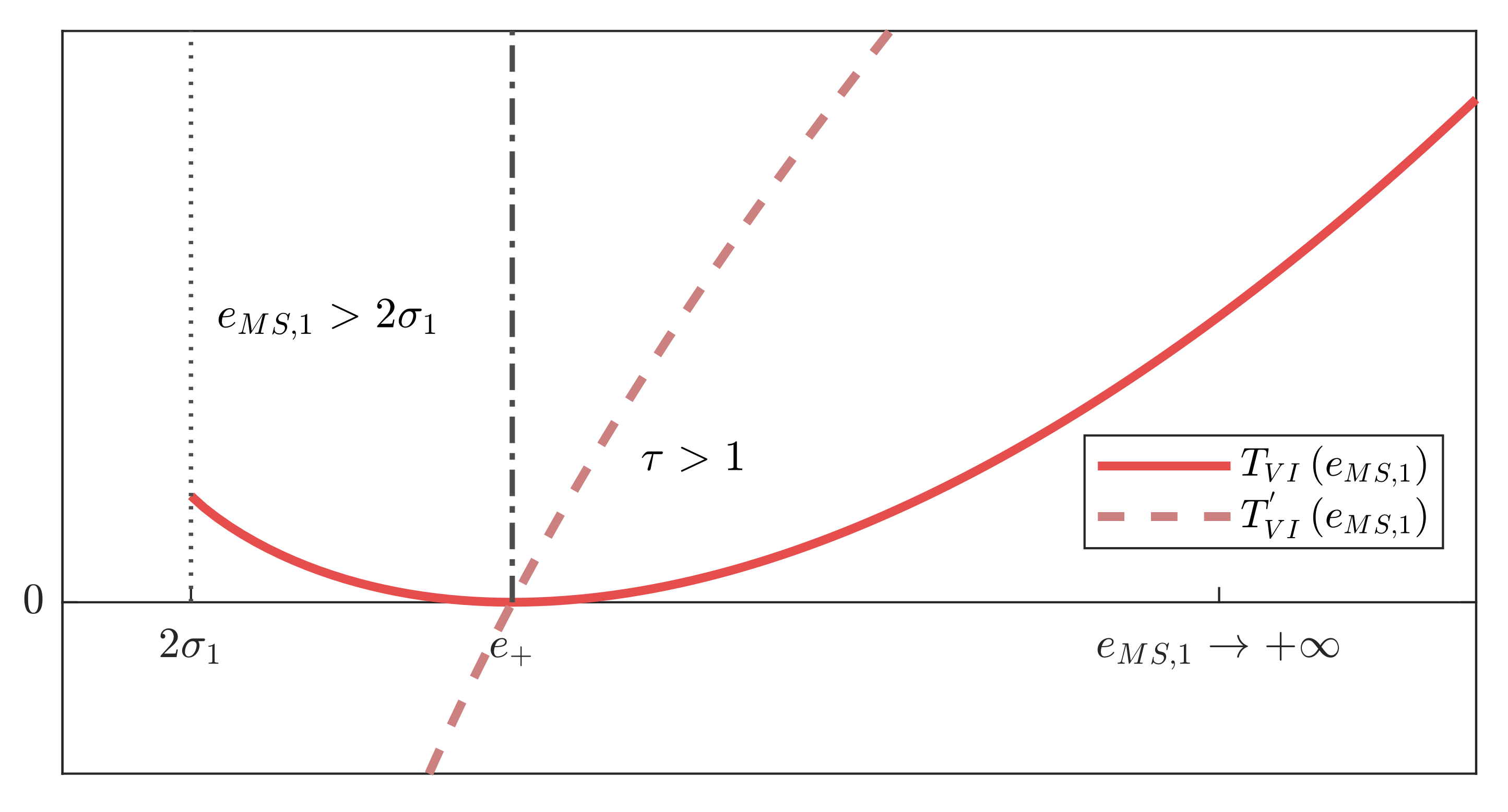
Figure 4 shows that (54) as a function of e ^ M S , 1 is monotone. A mathematical proof of monotony is given in the Appendix A. Thus, it is also monotone as a function of T M S and even strictly monotone for τ ^ 1 > 1 , which is the case that we are interested in. Therefore, the MS model and the VI model are fully equivalent for repeated observations to be tested for m = 1 outlier.
Finally, we numerically determine the probability distribution of test statistic (54) using Monte Carlo integration by
  • defining the ratio σ W / σ 1 ,
  • generating normally distributed pseudo random numbers for e M S , 1 ,
  • evaluating (53) and (54), and
  • taking the histogram of (54),
using 10 7 pseudo random samples of e ^ M S , 1 . In Figure 5, the positive branch of the symmetric probability density function (PDF) is given in logarithmic scale for various ratios of σ W / σ 1 . However, only about 30% of the probability mass is located under this curve, the rest is concentrated at T V I = 0 , and is not displayed. The quantiles of this distribution determine critical values and also α max in (19). The results are summarized in Table 1.

4.4. Variance Inflation Model—Test for Two Outliers

In the case m = 2 outliers, (35) reads
x ^ V I W = σ W 2 y 1 x ^ V I + σ W 2 y 2 x ^ V I .
The solution for x ^ V I can be expressed in terms of a cubic equation, which permits an analytical solution. One real solution must be in the interval y 1 y 2 , but there may be two more solutions
  • both below y 1 , if W < y 1 , or
  • both above y 2 , if W > y 2 , or
  • both between y 1 and y 2 , if y 1 > W > y 2 .
In rare cases, solutions may also coincide. The analytical expressions are very complicated and they do not permit a treatment analogous to the preceding subsection. Therefore, we have to fully rely on numerical methods, which, in our case, is the Monte Carlo method (MCM).
First, we compute the critical values of the test statistic (18)
T V I = 0 if max ( τ ^ 1 , τ ^ 2 ) 1 , ( x ^ V I w ) 2 σ w 2 2 + τ ^ 1 + τ ^ 2 log τ ^ 1 log τ ^ 2 otherwise .
The MCM is preformed, using 10 7 pseudo random samples. We restrict ourselves to the case σ 1 = σ 2 . The maximum selectable type 1 error probabilities α max are summarized in Table 2. It is shown that α max is mostly larger than for m = 1 . The reason is that, more often, we obtain τ ^ i > 1 , even if H 0 is true, which makes it easier to define critical values in a meaningful way. Moreover, Table 2 indicates the probabilities that under H 0
  • (16) has no local minimum, and if it has, that
  • max ( τ ^ 1 , τ ^ 2 ) 1
  • τ ^ 1 1 , τ ^ 2 > 1 or vice versa
  • min ( τ ^ 1 , τ ^ 2 ) > 1
i.e., none, one, or both variances are inflated. It is shown that, if the good observations contain the majority of the information, a minimum exists, but, contrary to our expectation, the case max ( τ ^ 1 , τ ^ 2 ) 1 is not typically the dominating case.
The important result is what happens, if H 0 is false, because variances are truly inflated. The probability that H 0 is rejected is known as the power 1 β of the test, where β is the probability of a type 2 decision error. It is computed both with T M S in (31) as well as with T V I in (59). Table 3 provides the results. It is shown that the power of T M S is always better than of T V I . This is unexpected, because T M S is not equivalent to the likelihood ratio of the VI model.
A possible explanation of the low performance of T V I in (59) is that, in many cases, the likelihood function L V I has no local maximum, such that (16) has no local minimum. Even for an extreme variance inflation of τ 1 = τ 2 = 5 this occurs with remarkable probability of 0.14. Moreover, the probability that max ( τ ^ 1 , τ ^ 2 ) 1 is hardly less than that. In both cases, H 0 cannot be rejected.

4.5. Outlier Identification

If it is not known which observations are outlier-suspected, a multiple test must be set up. If the critical values are identical in all tests, then we simply have to look for the largest test statistic. This is the case for T M S when considering the same number m of outlier-suspected observations, see (9). If we even consider different numbers m in the same multiple test, we have to apply the p-value approach, cf. Lehmann and Lösler [5].
In the VI model, the requirement of identical critical values is rarely met. It is, in general, not met for repeated observations, not even for m = 1 , as can be seen in Figure 5. However, in this case, it is no problem, because the test with T V I in (54) is equivalent to T M S in (30), as demonstrated. This also means that the same outlier is identified with both test statistics.
For repeated observations, we find identical critical values only for identical variances of the outlier-suspected observations, such that those observations are fully indistinguishable from each other. For example, for n = 27 , m = 2 , α = 0.05 , and σ 1 = = σ n , we find σ W / σ i = 0.20 and c α = 2.32 for all 351 pairs of outlier-suspected observations, see Table 2.
We evaluate the identifiability of two outliers in n = 10 and n = 20 repeated observations with m = 2 outliers while using the MCM. In each of the 10 6 repetitions, random observations are generated having equal variances. Two cases are considered. Whereas, in the first case, two variances are inflated by τ according to the VI model, in the second case, two observation values are shifted by ∇ according to the MS model. Using (31) and (59), the test statistics T M S and T V I are computed for all n ( n 1 ) / 2 = 45 or 190 pairs of observations. If the maximum of the test statistic is attained for the actually modified pair of observations, the test statistic correctly identifies the outliers. Here, we assume that α is large enough for the critical value to be exceeded, but otherwise the results are independent of the choice of α . The success probabilities are given in Table 4.
As expected, the success probabilities increase as τ or ∇ gets large. However, for both cases, T M S outperforms T V I . In Figure 6, the ratio r T of the success probabilities between the VI and the MS approach is depicted, having n = 10 repeated observations. If r T > 1 , the success rate of T V I is higher than for T M S and vice versa. The ratio is always r T < 1 and tends to 1, as shown in Figure 6. Therefore, the success probability of the MS is higher than for the VI approach, even if the outliers are caused by an inflation of the variances.

5. Conclusions

We have studied the detection of outliers in the framework of statistical hypothesis testing. We have investigated two types of alternative hypotheses: the mean shift (MS) hypothesis, where the probability distributions of the outliers are thought of as having a shifted mean, and the variance inflation (VI) model, where they are thought of as having an inflated variance. This corresponds to an outlier-generating process thought of as being deterministic or random, respectively. While the first type of alternative hypothesis is routinely applied in geodesy and in many other disciplines, the second is not. However, even if the VI model might be more adequate to describe the stochastics of the observations, this does not mean that it is possible to estimate parameters or detect outliers better than with some less adequate model, like MS.
The test statistic has been derived by the likelihood ratio of null and alternative hypothesis. This was motivated by the famous Neyman–Pearson lemma, cf. Neyman and Pearson [20], even though that this lemma does not directly apply to this test. Therefore, the performance of the test must be numerically evaluated.
When compared to existing VI approaches, we
  • strived for a true (non-restricted) maximization of the likelihood function;
  • allowed for multiple outliers;
  • fully worked out the case of repeated observations; and,
  • computated the corresponding test power by MC method for the first time.
We newly found out that the VI stochastic model has some critical disadvantages:
  • the maximization of the likelihood function requires the solution of a system of u polynomial equations of degree m + 1 , where u is the number of model parameters and m is the number of suspected outliers;
  • it is neither guaranteed that the likelihood function actually has such a local maximum, nor that it is unique;
  • the maximum might be at a point where some variance is deflated rather than inflated. It is debatable, what the result of the test should be in such a case;
  • the critical value of this test must be computed numerically by Monte Carlo integration. This must even be done for each model separately; and,
  • there is an upper limit (19) for the choice of the critical value, which may become small in some cases.
For the first time, the application of the VI model has been investigated for the most simple model of repeated observations. It is shown that here the likelihood function admits at most one local maximum, and it does so, if the outliers are strong enough. Moreover, in the limiting case that the suspected outliers represent an almost negligible amount of information, the VI test statistic and the MS test statistic have been demonstrated to be almost equivalent.
For m = 1 outlier in the repeated observations, there is even a closed formula (54) for the test statistic, and the existence and uniqueness of a local maximum is equivalent to a simple checkable inequality condition. Additionally, here the VI test statistic and the MS test statistic are equivalent.
In our numerical investigations, we newly found out that for m > 1 outliers in the repeated observations the power of the VI test is worse than using the classical MS test statistic. The reason is the lack of a maximum of the likelihood function, even for sizable outliers. Our numerical investigations also show that the identifiability of the outliers is worse for the VI test statistic. This is clearly seen in the case that the outliers are truly caused by shifted means, but also in the other case the identifiability is slightly worse. This means that the correct outliers are more often identified with the MS test statistic.
In the considered cases, we did not find real advantages of the VI model, but this does not prove that they do not exist. As long as such cases are not found, we therefore recommend practically performing outlier detection by the MS model.

Author Contributions

Conceptualization, R.L.; Methodology, R.L.; Software, R.L. and M.L.; Validation, M.L.; Investigation, R.L. and M.L.; Writing—Original Draft Preparation, R.L. and M.L.; Writing—Review & Editing, R.L., M.L., F.N.; Visualization, M.L.; Supervision, F.N. All authors have read and agreed to the published version of the manuscript.

Funding

This research received no external funding.

Conflicts of Interest

The authors declare no conflict of interest.

Appendix A

To prove the monotony of the tails of the function T V I e M S , 1 in (54), the extreme values of T V I have to be determined. Since T V I is symmetric, it is sufficient to restrict the proof for positive values of e M S , 1 . The first derivation of T V I is given by
T V I e M S , 1 = 4 σ W 2 σ 1 2 + 1 e M S , 1 2 σ 1 2 + σ W 2 + e M S , 1 σ 1 2 σ W 2 e M S , 1 2 4 σ W 2 σ W 2 σ 1 2 + σ W 2 e M S , 1 2 4 σ W 2 .
Setting T V I e M S , 1 = 0 yields two roots
e ± = ± ( σ 1 2 + σ W 2 ) σ 1 .
Inserting the positive extreme value e + into the second derivation of T V I , i.e.,
T V I e M S , 1 = e M S , 1 σ 1 2 + σ W 2 + e M S , 1 2 4 σ W 2 σ W 2 σ 1 2 σ W 2 σ 1 2 + σ W 2 e M S , 1 2 4 σ W 2 ,
identifies e + as a minimum value, because T V I e + is always positive for τ 1 > 1 , cf. (55). For that reason, T V I is a monotonically increasing function on the interval e + , + . Figure A1 depicts the positive tail of T V I and T V I , respectively, as well as the minimum e + .
Figure A1. Tail of the function T V I and its first derivation T V I for positive values of e M S , 1 as well as the minimum e + .
Mathematics 08 00991 g0a1

References

  1. Rofatto, V.F.; Matsuoka, M.T.; Klein, I.; Veronez, M.R.; Bonimani, M.L.; Lehmann, R. A half-century of Baarda’s concept of reliability: A review, new perspectives, and applications. Surv. Rev. 2018, 1–17. [Google Scholar] [CrossRef]
  2. Baarda, W. A Testing Procedure for Use in Geodetic Networks, 2nd ed.; Netherlands Geodetic Commission, Publication on Geodesy: Delft, The Netherlands, 1968. [Google Scholar]
  3. Teunissen, P.J.G. Distributional theory for the DIA method. J. Geod. 2018, 92, 59–80. [Google Scholar] [CrossRef]
  4. Lehmann, R. On the formulation of the alternative hypothesis for geodetic outlier detection. J. Geod. 2013, 87, 373–386. [Google Scholar] [CrossRef] [Green Version]
  5. Lehmann, R.; Lösler, M. Multiple outlier detection: Hypothesis tests versus model selection by information criteria. J. Surv. Eng. 2016, 142, 04016017. [Google Scholar] [CrossRef] [Green Version]
  6. Lehmann, R.; Lösler, M. Congruence analysis of geodetic networks—Hypothesis tests versus model selection by information criteria. J. Appl. Geod. 2017, 11. [Google Scholar] [CrossRef]
  7. Teunissen, P.J.G. Testing Theory—An Introduction, 2nd ed.; Series of Mathematical Geodesy and Positioning; VSSD: Delft, The Netherlands, 2006. [Google Scholar]
  8. Kargoll, B. On the Theory and Application of Model Misspecification Tests in Geodesy; C 674; German Geodetic Commission: Munich, Germany, 2012. [Google Scholar]
  9. Bhar, L.; Gupta, V. Study of outliers under variance-inflation model in experimental designs. J. Indian Soc. Agric. Stat. 2003, 56, 142–154. [Google Scholar]
  10. Cook, R.D. Influential observations in linear regression. J. Am. Stat. Assoc. 1979, 74, 169–174. [Google Scholar] [CrossRef]
  11. Thompson, R. A note on restricted maximum likelihood estimation with an alternative outlier model. J. R. Stat. Soc. Ser. B (Methodological) 1985, 47, 53–55. [Google Scholar] [CrossRef]
  12. Gumedze, F.N.; Welhamb, S.J.; Gogel, B.J.; Thompson, R. A variance shift model for detection of outliers in the linear mixed model. Comput. Stat. Data Anal. 2010, 54, 2128–2144. [Google Scholar] [CrossRef]
  13. Gumedze, F.N. Use of likelihood ratio tests to detect outliers under the variance shift outlier model. J. Appl. Stat. 2018. [Google Scholar] [CrossRef]
  14. Koch, K.R.; Kargoll, B. Expectation maximization algorithm for the variance-inflation model by applying the t-distribution. J. Appl. Geod. 2013, 7, 217–225. [Google Scholar] [CrossRef]
  15. Koch, K.R. Outlier detection for the nonlinear Gauss Helmert model with variance components by the expectation maximization algorithm. J. Appl. Geod. 2014, 8, 185–194. [Google Scholar] [CrossRef]
  16. Koch, K.R. Parameter Estimation and Hypothesis Testing in Linear Models; Springer: Berlin/Heidelberg, Germany, 1999. [Google Scholar] [CrossRef]
  17. James, G.; Witten, D.; Hastie, T.; Tibshirani, R. An Introduction to Statistical Learning: With Applications in R; Springer Texts in Statistics; Springer: New York, NY, USA, 2013. [Google Scholar] [CrossRef]
  18. Arnold, S.F. The Theory of Linear Models and Multivariate Analysis; Wiley Series in Probability and Statistics; John Wiley & Sons Inc.: New York, NY, USA, 1981. [Google Scholar]
  19. Lehmann, R.; Voß-Böhme, A. On the statistical power of Baarda’s outlier test and some alternative. Surv. Rev. 2017, 7, 68–78. [Google Scholar] [CrossRef]
  20. Neyman, J.; Pearson, E.S. On the problem of the most efficient tests of statistical hypotheses. Philos. Trans. R. Soc. Lond. Ser. A Contain. Pap. Math. Phys. Character 1933, 231, 289–337. [Google Scholar] [CrossRef] [Green Version]
  21. Lehmann, R. Improved critical values for extreme normalized and studentized residuals in Gauss-Markov models. J. Geod. 2012, 86, 1137–1146. [Google Scholar] [CrossRef]
  22. Sherman, J.; Morrison, W.J. Adjustment of an inverse matrix corresponding to a change in one element of a given matrix. Ann. Math. Stat. 1950, 21, 124–127. [Google Scholar] [CrossRef]
  23. Nocedal, J.; Wright, S.J. Numerical Optimization, 2nd ed.; Springer: New York, NY, USA, 2006. [Google Scholar] [CrossRef] [Green Version]
  24. Prussing, J.E. The principal minor test for semidefinite matrices. J. Guid. Control Dyn. 1986, 9, 121–122. [Google Scholar] [CrossRef]
  25. Gilbert, G.T. Positive definite matrices and Sylveste’s criterion. Am. Math. Mon. 1991, 98, 44. [Google Scholar] [CrossRef]
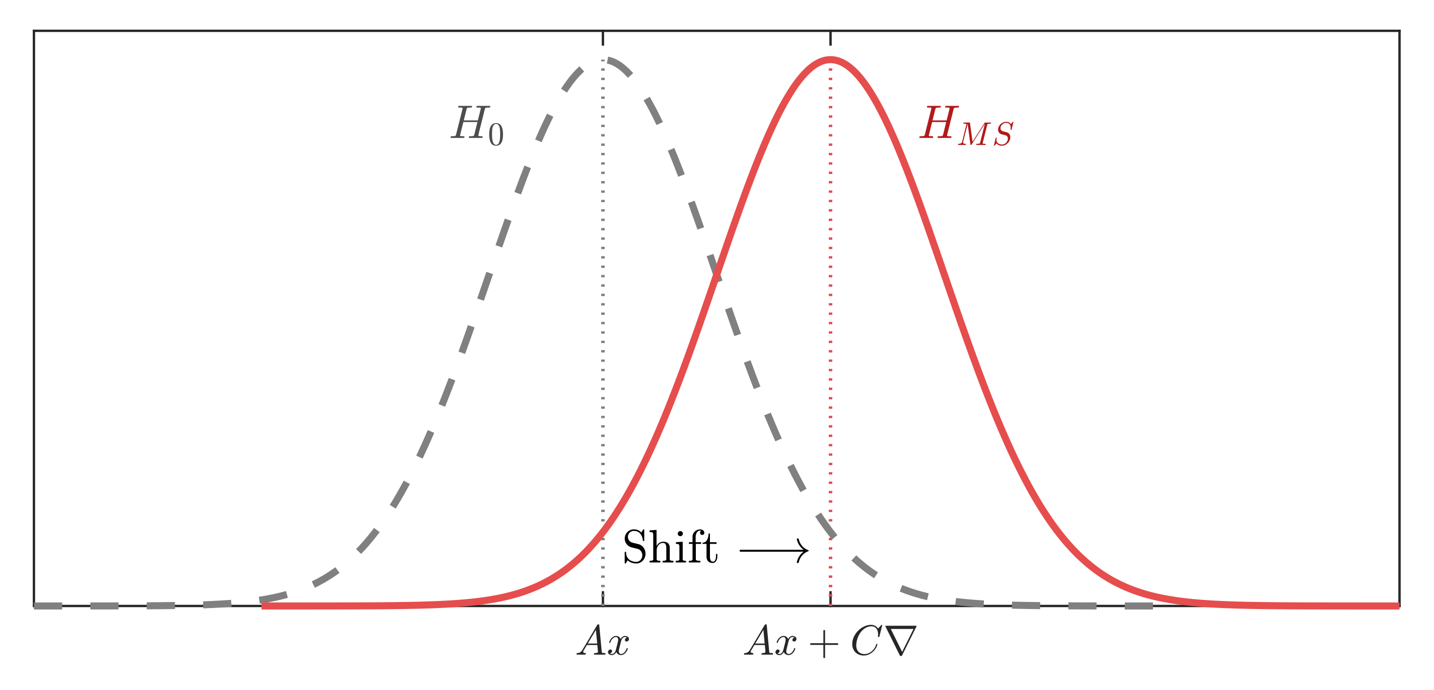
Figure 1. Schematic representation of the MS approach. The null model H 0 is depicted by a dashed grey line and the alternative model H M S is shown as a solid red line.
Mathematics 08 00991 g001
Figure 2. Schematic representation of the VI approach. The null model H 0 is depicted by a dashed grey line and the alternative model H V I is shown as solid red line.
Mathematics 08 00991 g002
Figure 3. Illustration of two exemplary cases of the solution of (35). Whereas the dash-dot red styled lines indicate the right hand side of the function, the black colored dashed line depicts the left hand side of (35). A dark red circle symbolises the desired solution out of five.
Mathematics 08 00991 g003
Figure 4. Resulting test statistic T V I of the variance inflation (VI) approach (54) as a function of the residual e ^ M S , 1 for various ratios of σ w / σ 1 .
Mathematics 08 00991 g004
Figure 5. Probability density function of T V I (54) as a function of the residual e ^ M S , 1 under H 0 , approximated by MCM. Vertical axis is in logarithmic scale. The strong peaks at 0 for τ ^ 1 1 are not displayed. The dashed black and the solid red curve relates to σ W / σ 1 = 0.05 and σ W / σ 1 = 0.5 , respectively.
Mathematics 08 00991 g005
Figure 6. Ratio r T of the success probabilities between the VI and the MS approach using n = 10 repeated observations. The top figure depicts r T for the case of inflated variances. The bottom figure depicts r T for the case of shifted mean values.
Mathematics 08 00991 g006
Table 1. Maximum selectable type 1 error probability α max and critical value c α for T V I in (54) for various ratios of σ W / σ 1 and α = 0.05 .
σ W / σ 1 α max c α
0.050.3171.50
0.100.3151.49
0.200.3081.47
0.300.2971.43
0.500.2641.33
Table 2. Maximum selectable type 1 error probability α max and critical value c α for T V I in (59) for various ratios of σ W / σ 1 = σ W / σ 2 and α = 0.05 as well as probabilities that (16) has no local minimum or that 0 or 1 or 2 variances are inflated.
Probabilities for
no012
σ W / σ 1 = σ W / σ 2 α max c α minInflated Variances
0.010.524.680.030.450.420.10
0.020.514.360.060.420.410.10
0.030.504.110.090.400.400.10
0.050.483.690.150.360.380.10
0.100.433.000.290.270.330.10
0.200.332.320.530.140.240.09
0.300.241.820.690.060.160.09
0.500.120.970.880.010.050.07
Table 3. Test power 1 β M S for test using T M S in (31) and test power 1 β V I for test using T V I in (59) for various true values of the variance inflation factors τ 1 , τ 2 for σ W = 0.1 · σ 1 = 0.1 · σ 2 and α = 0.05 , as well as probabilities that (16) has no local minimum or that 0 or one or two variances are inflated.
Probabilities for
Test Powerno012
τ 1 τ 2 1 β MS 1 β VI minInflated Variances
1.01.00.050.050.290.270.330.10
1.21.20.080.080.270.240.350.13
1.51.50.130.120.240.210.380.17
2.02.00.220.200.210.170.390.23
3.03.00.360.320.180.120.390.31
5.05.00.550.490.140.080.360.42
1.01.50.090.090.270.240.360.13
1.03.00.210.190.240.180.410.18
2.03.00.300.260.190.140.400.27
2.05.00.400.360.180.110.400.31
Table 4. Success probabilities for outlier identification in repeated observations of equal variance σ 2 with two outliers.
Success Probabilities for n = 10 Success Probabilities for n = 20
τ 1 = τ 2 of T MS in (31)of T VI in (59)of T MS in (31)of T VI in (59)
1.00.0220.0210.0050.005
2.00.0650.0610.0280.026
3.00.1080.1040.0610.057
4.00.1500.1440.0950.089
5.00.1850.1800.1280.121
6.00.2180.2120.1560.151
1 = 2 of T MS in (31)of T VI in (59)of T MS in (31)of T VI in (59)
0.00.0220.0210.0050.005
1 σ 0.0810.0650.0350.028
2 σ 0.3250.2860.2260.202
3 σ 0.6830.6520.6060.586
4 σ 0.9120.9020.8920.886
5 σ 0.9850.9840.9840.984