1. Introduction
Wind energy based electrical generation has undergone important growth during the last decade. According to a report by the association WindEurope [
1], the cumulative capacity of the wind energy raised from nearly 60 GW in the year 2008 to around 180 GW in the year 2018, which depicts an increment of 200% in 10 years. Additional information about important growth of the wind energy in different countries can also be found in the literature [
2,
3]. In the same way, nowadays there are many wind turbine manufacturers and, according to the Global Wind Energy Council [
4], around 341.320 wind turbines were operating all over the world at the end of 2016. All of these turbines have different structural characteristics or operate in different conditions.
An important issue during the design process of a wind turbine is the design of its control system. These control algorithms regulate the performance of the wind turbine during the whole range of operating conditions, mainly responding to a double functional objective: regulation of the generated electrical power (maximization for under rated wind speed conditions and saturation for above rated wind speed conditions) and minimization of the mechanical loads in the structural elements of the wind turbine (tower, blades and power shaft).
The regulation of the performance of a wind turbine is usually achieved with two different control loops: the torque control loop and the pitch control loop, see Bianchi et al. [
5]. The torque control loop, as explained in the work of Burton et al. [
6], regulates the rotational speed of the rotor of the wind turbine when the system in under rated condition. To that end, the electromagnetic torque of the electrical generator is modified by means of a power electronics converter. The pitch control loop, as explained in the work of Bossanyi et al. [
7], regulates the rotational speed of the wind turbine when the system is in rated condition. The actuator associated to this control loop is the pitch system, which allows for modification of the Angle of Attack (AoA) of the incoming relative wind with respect to the blades of the wind turbine. Hence, the power extracted from the wind can be regulated.
The effect of the pitch system in the performance of the National Renewable Energies Laboratory (NREL) 5 MW wind turbine is presented by Jonkman et al. [
8]. According to their explanation, the pitch system has two important characteristics to be taken into account: a negative sensitivity with respect to the aerodynamic power and a high non-linearity, which arises as a result of the different effect of the pitch angle variations at non-identical operating points. An analysis of the interdependency between the pitch system response and the operating point of the wind turbine is presented in the work of Muhando et al. [
9].
The most important requirement during the design of the control system of a wind turbine is the guarantee of the stability of the control loops. The most widely-used techniques for the assessment of the stability are the Routh-Hurwitz (RH) and the Gain Phase Margin (GPM) methods. The RH criterion [
10,
11], proposed by E.J. Routh and A. Hurwitz in 19th century, provides a way to study the absolute stability of a system. The stability criterion used by the Routh Hurwitz method, as it is explained in the work of Choghadi et al. [
12], is that no roots of the characteristic polynomial of the closed loop system are located in the Right Half Plane (RHP). The GPM method [
13,
14] defines the relative stability of a system according to the value of the Gain Margin (GM) and the Phase Margin (PM), being the latter usually linked to the damping of the system. In order for a system to be stable, the GM and the PM have to be positive. The GPM method can be evaluated numerically (Ho et al. [
14]), with the Nyquist plot (Ho et al. [
15]) or by means of the Bode plot (Cavicchi et al. [
16]).
However, one of the problems linked to the methods explained before is their lack of capability to deal with the uncertainties. In fact, it is known that many systems may present uncertainties that modify the characteristics of the plant, and thus compromise the stability of the system. Variation of the characteristic of the wind turbine, fabrication tolerances or non-linearities related to different operating-points may be the sources of the uncertainties. In this context, in order to minimize the effect of the uncertainties in the performance of the designed controllers, different robust control strategies and stability analyses can be found in the literature. Yuan et al. [
17] present in their work a robust H
inf based controller for the individual pitch control of a wind turbine. The robust control of the Doubly Fed Induction Generator (DFIG) of a wind turbine is covered in the works of Muhando et al. [
18] and Surinkaew et al. [
19].
In line with the design of robust controllers, robust stability analysis methods can also be found in the literature. The principal robust stability criteria are the Sylvester or Lyapunov Equations (SLE) and the Kharitonov analysis. The SLE based criterion assesses the stability of time-varying dynamic systems; see Amato et al. [
20]. As explained in the work of Behr et al. [
21], the Lyapunov Equation is the symmetric version of the general Sylvester Equation, so they are usually considered to be part of the same criterion. The application of the Lyapunov criterion to the control system of a horizontal axis wind turbines can be found in the works of Palejiya et al. [
22,
23]. In those papers, the stability of a control algorithm proposed for the transitions of the wind turbine between the under rated and the rated operations is analyzed by means of the Lyapunov criterion. Bennouk et al. [
24] carry out a Lyapunov based stability analysis of the DFIG system of a wind turbine.
The Kharitonov theorem [
25,
26] claims that the stability of a system with uncertainties can be guaranteed if the individual stability of 4 Kharitonov polynomials is proven. To that end, the systems with the uncertainties are calculated and defined by means of their characteristic polynomial and the upper and lower limits of the coefficients are considered to infer the Kharitonov polynomials. In the work of Veronica et al. [
27], the Kharitonov theorem is used to evaluate the stability of a controller implemented in a microgrid. In the same way, in the work of Raouf et al. [
28], the Kharitonov theorem is used to evaluate the stability of a controller in a hybrid wind-diesel generation system. Finally, in the work of Ahmed et al. [
29], the Kharitonov robust stability analysis is used to evaluate the absolute stability of the pitch control loop of a wind turbine simplified model. Nevertheless, no robust stability analysis based on the Kharitonov theorem and applied to a complex and realistic wind turbine model has been found in the literature.
Hence, in this paper, the Kharitonov theorem is applied to the stability analysis of the pitch control system of the NREL 5 MW horizontal axis wind turbine, which is widely considered to be a reference wind turbine for many kinds of analyses. A detailed description of the characteristics of the NREL 5 MW wind turbine is presented in the work of Jonkman et al. [
8]. Moreover, regarding classification of the wind turbine according to the criteria proposed by the International Electrotechnical Commission (IEC), the NREL 5 MW wind turbine belongs to the class IIA, see Kim et al. [
30]. For the modelling of the pitch control system of the wind turbine, the linearization tool of the open-source aeroelastic code FAST v7 [
31] has been used, which has been designed by the NREL. By using the linearization tool included in FAST v7, highly detailed models of the wind turbine at many operating points can be calculated.
The objective of the analysis proposed in this paper is to evaluate the viability of the Kharitonov theorem when assessing the stability of a pitch controller of a wind turbine subjected to uncertainties due to variations in its operating conditions. Moreover, it is to be evaluated if the complexity and degree of detail of the wind turbine model used in the analysis, as well as the deviation in the operating conditions, may compromise the correct performance of the Kharitonov theorem. In consequence, different order wind turbine models and many deviations in the operating point are to be used in the stability analysis.
This paper is structured as follows: In
Section 2 the procedure for the modelling of the pitch control system with the aeroelatstic code FAST v7 is presented. A detailed explanation of the Kharitonov robust stability analysis is given in
Section 3. In
Section 4, the procedure for the application of the Kharitonov theorem to the pitch control system of the NREL 5 MW wind turbine is introduced. Finally, the results and discussion and the conclusions are presented in
Section 5 and
Section 6, respectively.
2. Modelling of the Pitch Control System
The pitch control loop of a horizontal axis wind turbine regulates the rotational speed of the rotor when the system is in rated condition, i.e., when the value of the wind speed is high enough to keep the power produced by the wind turbine at rated value. To that end, the pitch angle of the wind turbine blades is modified by means of an electrical or hydraulic system. As a consequence, the AoA of the incident relative wind is also modified and the aerodynamic power that the wind turbine extracts from the wind can be limited.
An illustration of the pitch angle and the AoA of the wind during the rotation of the wind turbine blade is shown in
Figure 1. Note that
refers to the pitch angle of the wind turbine blade,
refers to the twist angle of the wind turbine, AoA refers to the angle of attack of the incident relative wind and
refers to the value of incident relative wind speed.
While some simplified models representing the effect of the pitch angle on the dynamic performance of the wind turbine at different operating points can be developed, the most accurate choice to study this topic is the use of aeroelastic codes. Aeroelastic codes are formed by a high number of equations that represent the operation of the different components of the wind turbine (tower, power shaft, blades, nacelle and foundation) with a high degree of accuracy. Hence, the results obtained with these aeroelastic codes can be more easily extrapolated to real wind turbines.
The aeroelastic code used for the analysis presented in this paper is FAST v7 [
31]. An important characteristic of FAST v7 is that it does not only allow to carry out non-linear simulations of the operation of the wind turbine, but also to calculate linear models at different operating points. Hence, in order to characterize the effect of the pitch angle on the dynamic performance of the wind turbine at different operation conditions, the linearization tool of the aeroelastic code FAST v7 has been used to obtain linear models of the wind turbine at various operating points. The operating points considered have been listed in
Table 1.
As a result of the linearization process, a Linear Time Invariant (LTI) system in state-space form is obtained, see Equation (1).
where:
is the state matrix and represents the dynamics of the system
is the input matrix
is the output matrix
is the feedforward matrix
is the matrix that contains the states of the system
is the matrix that contains the derivatives of the states of the system
is the input variable. The pitch angle in this case.
is the output variable. The rotational speed of the generator in this case.
In the analysis presented in this paper, the LTI models of the wind turbine at each one of the operating points listed in
Table 1 have been calculated. As it was expected, due to the characteristic of non-linearity of the pitch angle in the performance of the wind turbine, the location of the poles and zeros of the LTI model varies considerably for each one of the operating points, see
Figure 2, which results in an alteration of the dynamics of the system. As a result, the sensitivity of the rotational speed of the generator with respect to variations of the pitch angle is expected to vary considerably depending on the operating conditions as well.
In presence of such non-linearities, the Kharitonov robust stability theorem seems to be a good option to analyze the stability of a pitch controller in a determined range of operating conditions of the wind turbine. Moreover, the use of the aeroelastic code FAST v7 to calculate the linear model ensures its mathematical accuracy and realistic representation of the reality.
A flowchart depicting the main steps of the linearization and pitch control system model calculation process is presented in
Figure 3.
3. Kharitonov Robust Stability Theorem
The Kharitonov robust stability theorem, first introduced by V.L. Kharitonov [
25] in 1978, is a mathematical proposition aimed to analyze the stability of a system in case of uncertainties or dynamic variations of its parameters. The variation of the parameters may be due to different reasons, such as, non-linearities inherent to the nature of the system, changes in the operating conditions or non-expected variations of its physical components. As it has been proven in
Section 2, the dynamics of the pitch system of a wind turbine are highly non-linear, showing remarkable differences in the location of the poles at variable operating conditions. As a result, the pitch system of a wind turbine is considered to be a suitable candidate to be studied by the Kharitonov robust stability theorem. Consequently, the first step is to obtain the open-loop transfer function of the system to be studied, see
Section 2, and present it as shown in Equation (2).
As the controller, a classical Proportional-Integral (PI) topology is selected, see Equation (3).
For the whole analysis, the proportional and integral gains are defined as
and
. Note that the negative signs responds to the negative sensitivity of the power produced of the wind turbine with respect to variations in the pitch angle. Even if the most common strategy for the pitch control loop design is the Gain Scheduling [
32], in this case, the controller gains have been fixed and it has been ensured that the closed loop response of the system with the proposed controller gains, and at each one of the operating points, is stable. The objective of keeping fixed valued controller gains is to reduce the sources of non-similarities between models.
Once the expression of the open loop plant and the controller are known, the characteristic polynomial of the closed loop transfer function can be calculated as shown in Equation (4).
Finally, the characteristic polynomial must be transformed into the form of an interval polynomial, see Equation (5).
where each coefficient is supposed to take a value within a defined range, i.e.,
. This range is derived from the uncertainties or dynamic variations of the parameters of the system.
In this case, various plants corresponding to different operating conditions of the wind turbine have been obtained using the linearization tool of FAST v7. By following the procedure presented from Equations (2)–(5) for each one of the LTI models obtained, the lower and upper limits of each one of the coefficients can be easily obtained. Once the limits
for each one of the parameters have not been obtained, the Kharitonov polynomials, shown in Equation (6) and first cited by V.L. Kharitonov [
25], can be calculated. According to the Kharitonov robust stability theorem, the stability of the system (with all the uncertainties considered) is guaranteed if the following 4 polynomials, also known as the Kharitonov polynomials, are stable on their own. The most widely used criterion to determine the stability of each Kharitonov polynomial is the Routh-Hurwitz theorem [
10,
11,
33].
In the work of Ahmed et al. [
29], the Kharitonov robust stability theorem is used to analyze the stability of the pitch control system of a wind turbine. Nevertheless, in the cited paper, a rather simple model of a wind turbine, with no consideration of the dynamics of the tower and the low speed shaft has been used. Hence, the obtained results could not be easily applicable to a real wind turbine. To overcome that, in this paper, instead of a simplified model, a realistic model with all the interactions and cross-couplings between all the elements of the wind turbine is used for the analysis. The objective is to assess the applicability of the Kharitonov theorem to be used with a complex and highly detailed model of a horizontal axis wind turbine.
4. Kharitonov Stability Analysis of the Pitch Control System
In this paper, a robust stability analysis, based on the Kharitonov stability theorem, of the pitch control system of the NREL 5 W wind turbine is carried out. Thus, the LTI models of the wind turbine at different operating conditions have been obtained as presented in
Section 2. It is to be highlighted that the proposed stability analysis is not restricted to be used with the pitch control system of a wind turbine, but it could be applied to any other system whose dynamics are known or measurable. Two concepts related to the Kharitonov theorem are considered of great importance when it comes to study the stability of the LTI systems: The order of the LTI models and the relative stability. Further explanations of both these concepts are given in the following subsections.
4.1. Model Order
As it was stated in
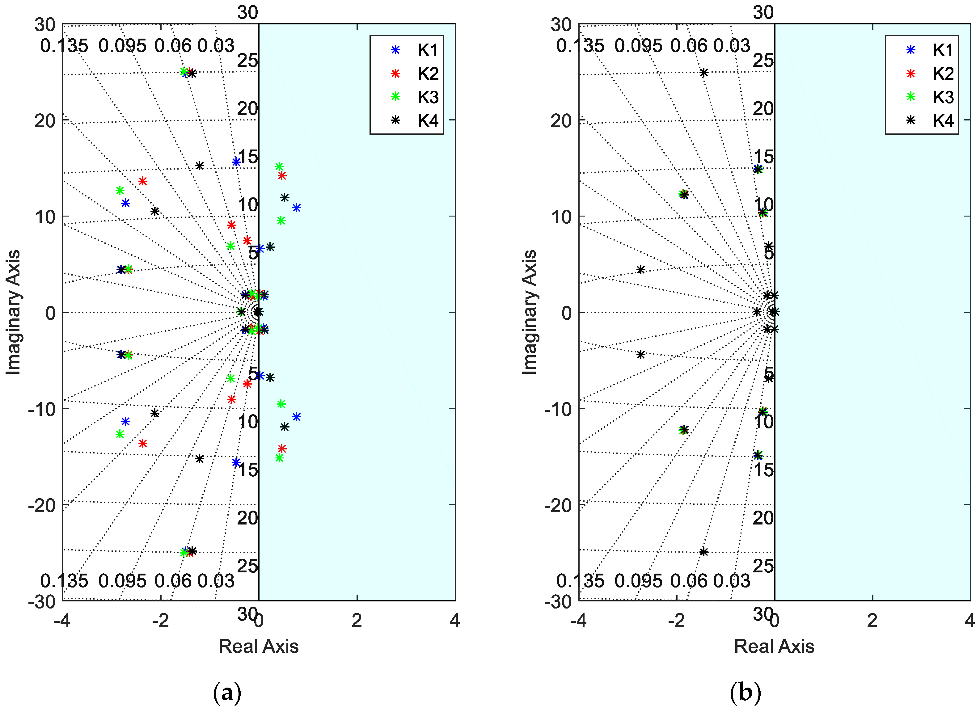
Section 3, the most widely used technique to assess the stability of the Kharitonov polynomials is the Routh-Hurwitz theorem. This theorem affirms that a system is stable if and only if all the poles of the interval polynomial have a negative real part. In this case, even if the LTI models from which the limits of the coefficients have been obtained are known, the location of the poles of the Kharitonov polynomials shown in Equation (6) will be totally unpredictable. To achieve a better understanding of that topic, the effect of increasing the order of the LTI model on the relocation of the poles of the Kharitonov polynomials is to be studied in this paper. Theoretically, the risk of instability of the systems is expected to rise with the increase of the order of the model.
On the one hand, as can be observed in
Figure 2, the complex model of the wind turbine presents open loop poles that are very close to the imaginary axis, which means they are easily susceptible to fall into instability when closing the loop. That must be taken into account, as the majority of the simplified models of a wind turbine found in the literature do not have such poles. Hence, the importance of working with a complex model to achieve realistic conclusions is highlighted.
On the other hand, models of such complexity have the drawback that the many existent interactions and cross-couplings between the poles can lead the system to instability. A study to determine the variation of the coefficients of the characteristic polynomial for different order models is carried out in this paper. Moreover, it must be understood that this analysis is essential when applying the Kharitonov stability theorem, because as shown in Equation (6), the Kharitonov polynomials consider situations of the wind turbine that are mathematically possible, but almost certainly not feasible in reality. Hence, a mathematically possible but really unfeasible situation could cause the Kharitonov theorem to assess an instability that is not going to happen in reality. A mathematical approach to this issue is presented from Equations (7)–(12). First, the characteristic polynomial of a closed loop system of order
is written as shown in Equation (7).
In order to guarantee the stability of the system, the classical Routh-Hurwitz method indicates that the characteristic polynomial must be equaled to 0, see Equation (8), and the location of the closed loop poles analyzed.
As it was previously stated, when doing a Kharitonov based stability analysis, it is important to study the variation of the characteristic polynomial with respect to the variation of its coefficients. Since both, the value of the coefficients and the location of the poles, are known to be dependent on the value of the coefficient, the derivative of the characteristic polynomial with respect to the coefficients can be expressed as shown in Equation (9).
From Equation (9), the sensitivity of the location of the poles with respect to variations of the coefficients of the characteristic polynomial can be calculated, see Equation (10).
If the sensitivity of the coefficients of the characteristic polynomial with respect to the pitch angle variation is introduced to the equation, the sensitivity of the poles with respect to the pitch angle variations can be calculated, see Equation (11). The sensitivity of the coefficients of the characteristic polynomial with respect to pitch angle variations could be easily computed by linearizing at different operating conditions, as it has been explained in
Section 2, and obtaining the characteristic polynomial associated to each case. The value of the coefficients of the characteristic polynomial for the LTI model corresponding to a wind speed of 19 m/s (Plant 4 in
Table 1) are shown in
Table 2.
Finally, from Equation (11) the variation of the poles with respect to variations of the pitch angle can be derived as shown in Equation (12).
As it can be concluded from Equations (11) and (12), the effect of the pitch angle variations on the location of the closed loop poles increases with the increment of the order of the model. There are two facts that suggest this:
- -
The variation of the coefficients of the characteristic polynomial with respect to the variations of the pitch angle, i.e.,
, will be bigger in case of high order polynomials, see
Table 2.
- -
The number of coefficients is higher in case of high order polynomials. Thus, the accumulative effect presented in Equation (11) will be more important.
As a result, it is to be expected that the Kharitonov stability theorem will be more prone to instability by considering high order plants. In this paper, an analysis to prove the difference in the sensitivity of distinct order models to variations in the pitch angle is presented. Moreover, the effect of this sensitivity on the performance of the classical Kharitonov stability theorem is also to be analyzed. To that end, the characteristic polynomials have been reduced to smaller orders. The square root method has been used for the reduction of the original LTI models. As it is explained in the works of Varga et al. [
34,
35], the square root method based reductions are performed via numerical computations and are known for their capability to make appropriate approximations based on the whole frequency range. The coefficients of the characteristic polynomial of different order plants corresponding to the LTI model calculated with a wind speed of 19 m/s (Plant 4 in
Table 1) are presented in
Table 2.
Note that the coefficient
, due to its very small value in comparison to the rest of the coefficients, has not been included in
Table 2 nor in the following tables presented in this paper.
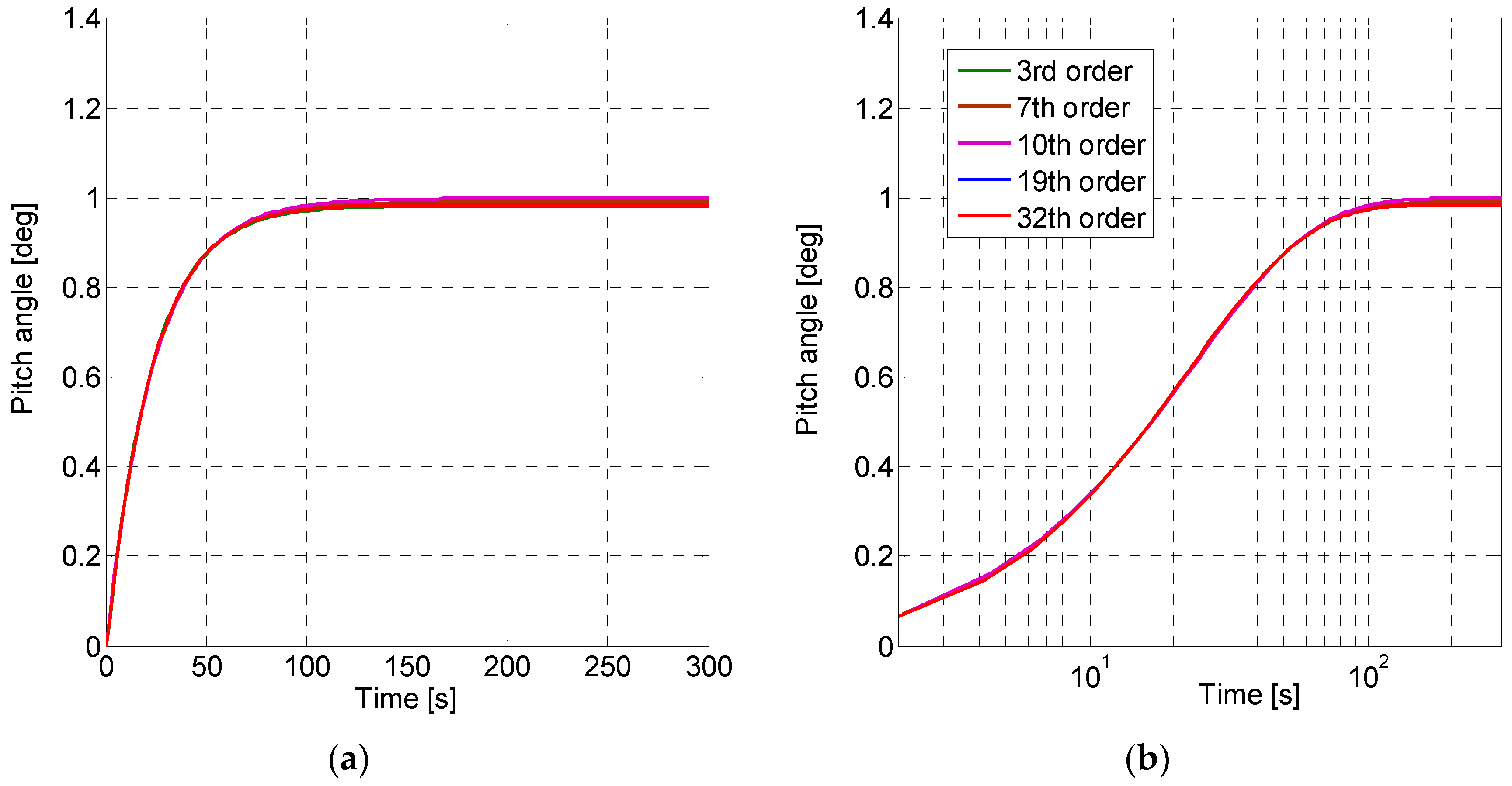
In order to ensure that the reduced plants have been obtained correctly, the step response of each one of them has been represented in
Figure 4. As it can be observed, all the plants present the same transient response, which indicates that the dynamics of the model have been maintained even if the order of the plant has been reduced. Moreover, the unity value of the steady state response ensures the correct performance of the closed loop control loop and the stability of the systems.
As can be seen in
Table 2, the values of the coefficients of the characteristic polynomial are remarkably bigger in case of high order models, and, thus, according to Equation (11), the sensitivity of the closed loop poles with respect to the variations in the pitch angle is expected to be bigger as well. Moreover, as big variations of the coefficients of the characteristic polynomial are expected to lead the system to instability, a new method to determine the lower and upper values of the coefficients of the Kharitonov polynomial is proposed in the analysis presented in this paper, see Equation (13).
where
is a factor to limit the maximum variation of the coefficients to be used in the Kharitonov polynomials and
is the intermediate or mean value of the coefficient with the uncertainties considered. The subscript
defines the number of the Kharitonov polynomial coefficient, being
the order of the polynomial.
The use of the factor is expected to enable to prove that the big variation of the coefficients is the responsible for the poor performance of the Kharitonov robust stability theorem with high order wind turbine models. By limiting the maximum and minimum values of the coefficients, the results should tend to stability. On the contrary, in low order models, being the interactions and cross-couplings between the poles less significant, the dependency on the factor should be non-existent or very small.
4.2. Relative Stability
The strength of the Kharitonov theorem lies in its ability to analyze the stability of systems that present uncertainties on their dynamic performance, which makes it a very powerful tool for robust system analysis. Nevertheless, one of the weaknesses associated to this theorem could be the lack of relativity in the assessment of the stability. Since the stability of the Kharitonov polynomials is analyzed by means of the Routh-Hurwitz theorem, only the absolute, and not the relative, stability of the system is determined. That means that the theorem only affirms if the system is stable or not, but not in which degree. To solve that issue, in this paper a new functionality is introduced to the original Kharitonov theorem, being the objective to offer the possibility to study the relative robust stability of the system.
The main idea behind the proposed functionality is the automatic variation of the coefficients of the characteristic polynomial, which will be calculated with respect to a different ordinate axis. The new ordinate axis is considered by shifting the original one, and, thus, by studying the absolute stability with respect to shifted ordinate axes, the relative stability with respect to the original one can be determined. The expression of the original characteristic polynomial is presented in Equation (7). The new characteristic polynomial would be calculated as shown in Equation (14).
where
indicates the location in the coordinate axis to which the new ordinate axis is shifted.
The mathematical procedure to calculate the coefficients of the new polynomial can be expressed as in Equation (15).
where
is the value of original coefficient and
is known as the binomial coefficient.
The expression corresponding to the binomial coefficient is presented in Equation (16).
where
and
are both integers and must satisfy the following condition
.
If the ordinate axis is shifted various distances defined by the parameter
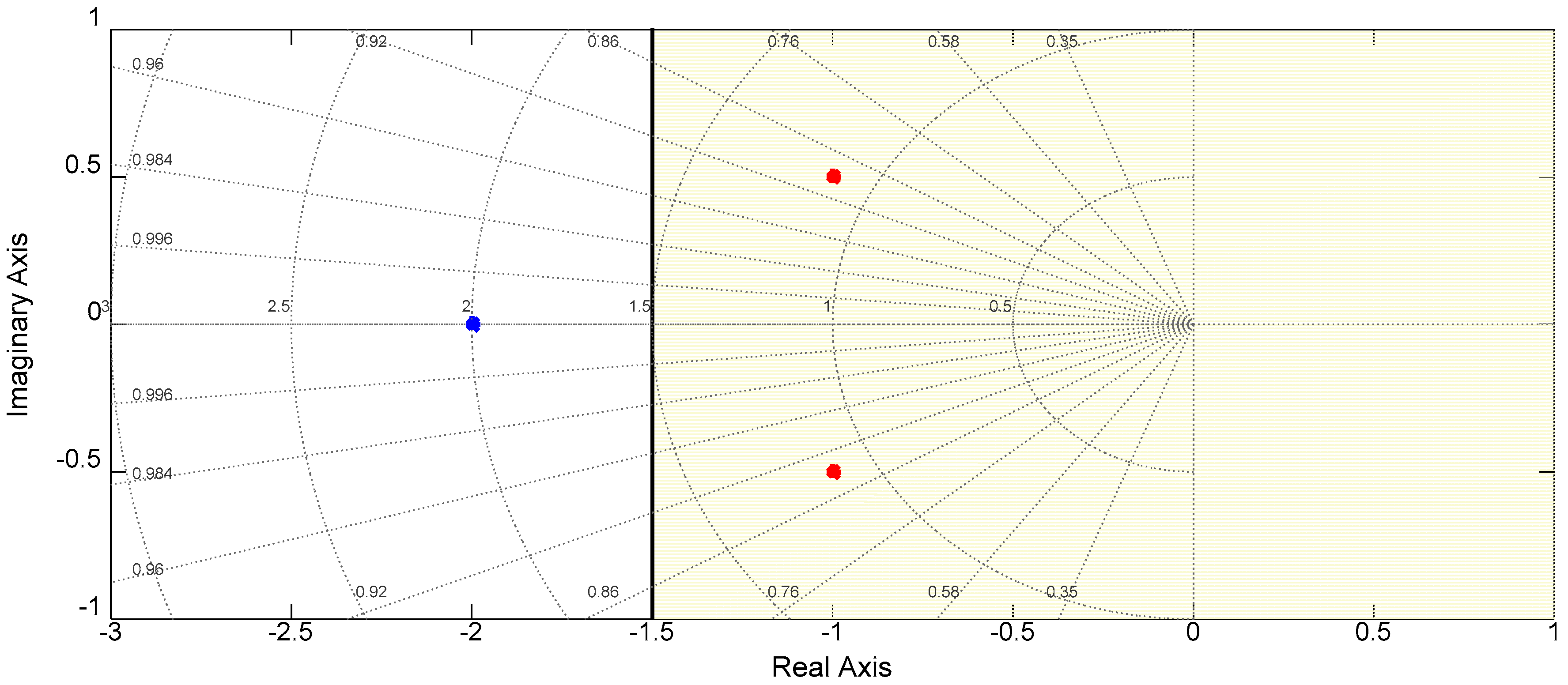
, the Kharitonov theorem will calculate the absolute stability with respect to the new requirements, and the relative stability of the system will be determined An illustrative example is shown in
Figure 5, where as a result of the shift of the ordinary axis to
, a couple of poles that were stable according to the classical stability theorem, are observed to be unstable with respect to the new axis, which means that they do not fulfill the relative stability requirement.
The coefficients of the characteristic polynomials of the LTI model, corresponding to a wind speed of 19 m/s (Plant 4 in
Table 1), and calculated with respect to new ordinate axes, placed in
and
, are presented in
Table 3 and
Table 4, respectively.
As can be observed by comparing the values presented in
Table 2,
Table 3 and
Table 4, the values of the coefficients of the characteristic polynomial differ as a result of the shift of the ordinate axis. Moreover, as it could be expected due to the bigger shift of the ordinate axis, the difference of the coefficient values between
Table 2 and
Table 3 is remarkably higher than between
Table 2 and
Table 4. Additionally, it is to be observed that the difference between the values of the coefficients is more easily noticeable in reduced order models, in which the required decimal precision for the presentation of the coefficient values is lower.
In any case, the calculation of the new polynomials with respect to the shifted ordinate axes is performed via a computationally simple operation, which makes its implementation straightforward. The proposed functionality could result of great utility for 2 important applications:
- -
The design of a controller that meets a more restrictive stability requirement.
- -
Check that a control system fulfills a relative stability requirement.
6. Conclusions
In the analysis presented in this paper, the Kharitonov robust stability criterion is applied to the pitch control system of the NREL 5 MW wind turbine. Due to the non-linear nature of the pitch system of a wind turbine, the variations of the operating conditions may cause uncertainties in the performance of the system. Hence, it is a suitable system to be studied by the Kharitonov robust stability analysis. In order to limit the sources of uncertainties, constant gains of the controller of the pitch control loop have been considered.
The first conclusion to be extracted from the analysis presented herein is that the complexity of the LTI model of the pitch system and the performance of the Kharitonov criterion are strongly related. As the complexity of the pitch model increases, the pole displacement of the Kharitonov polynomials increments, and that leads to a nonfulfillment of the Kharitonov stability criterion. Thus, a high order pitch model may be a very detailed representation of the reality, but not a good option for the Kharitonov theorem, since the existence of a high number of mathematically possible but physically unfeasible combinations of coefficients lead to a nonfulfillment of the robust stability criterion. An order reduction of the complex pitch system model is contemplated as a good option. On the one hand, the performance of the Kharitonov analysis is not so strongly affected by the mathematically possible but physically unfeasible coefficient combinations. On the other hand, compared to other simplified models seen in the literature, the reduced order pitch system models keep the dynamics of a detailed and realistic model of a horizontal axis wind turbine.
Furthermore, a procedure to complement the Kharitonov robust stability theorem with a relative stability analysis has been proposed and successfully tested in this paper. The result shows that this functionality could be particularly useful for undertaking the design of a controller subject to a certain relative stability requirement and with very little computational effort.
Finally, it is to be concluded that the Kharitonov robust stability theorem is considered to be a powerful mathematical tool and interesting option to study small deviances from an operating point. However, when it comes to covering wide ranges of operating points, it is not considered to be the best option because the consideration of physically unfeasible models could lead the designer to inaccurate conclusions.

 ,
, 


