Qualitative Study of a Well-Stirred Isothermal Reaction Model

Abstract

We consider a two-dimensional system which is a mathematical model for a temporal evolution of a well-stirred isothermal reaction system. We give sufficient conditions for the existence of purely imaginary eigenvalues of the Jacobian matrix of the system at its fixed points. Moreover, we show that the system admits a supercritical Hopf bifurcation.

1. Introduction

In the recent years mathematical studies of chemical, biological and biochemical systems are growing. There is a significant role played by limit cycles oscillations in biochemical reaction systems organization in living organisms and it is important to determine the simplest, realistic mechanisms that can generate periodic oscillations. Results on Hopf bifurcations of many systems, from two-dimensional, e.g., [1,2], to three dimensional, e.g., [3,4] or higher are known. Studies of limit cycles of a two-dimensional system, which is a mathematical model for a temporal evolution of a well-stirred isothermal reaction system in contact with a large bath,

$$\begin{array}{cc}\hfill \dot{x}=& a-xy+y^2,\hfill \\ \hfill \dot{y}=& (b-cy{(1+y)}^{-1}+xy-y^2)/K,\hfill \end{array}$$

(1)

go more than forty years back. The system in the form (1) was first time studied more detailed in [5], but some results are known as given as well by Z. Kadas and H.G. Othmer, see [6]. They have shown that a stable limit cycle can exist in a two-species open system. For such systems only one biomolecular reaction following mass action kinetics occurs. The disagreement with the results from paper [6] was then presented and supported with proofs in [5]. As written in paper [5], the authors in [6] claim that their choice of chemical potential differences for the constitutive relation is more appropriate on the thermodynamic grounds than a relation linear in concentration differences. The author J.J. Tyson disagree with that claim and presents arguments, and more details on the contradistinguished conclusion, that confirm his claim. Independently, the same results were obtained by Hanusse [7] and by Tyson and Light [8].

In the model presented by a system (1) are $a=(A/V)j_x$ and $b=(A/V)j_y$, where A is the area across which the diffusion takes place. The volume of the reaction vessel is denoted by V and $j_s$ is the flux of the species s into the vessel from the bath, K denotes the equilibrium constant for the reaction $x+y\rightleftharpoons 2y$ and c is a reaction rate. If the diffusional flux is given by

$$j_s=h_i({\mu }_s^0-{\mu }_s),$$

where ${\mu }_s$ and ${\mu }_s^0$ are the chemical potentials of species s (in our case dynamical quantities x and y) in the reaction vessel and in the bath, and $h_s$ is a “phenomenological coefficient”.

In this paper we performed a detailed study of of the behaviour of the vector field in the first quadrant. There we have observed more complicated behaviour of trajectories near singularity at the infinity, which was studied using blow-up method. For more details on this method, see [9]. We have determined all the singular points of system and studied the Hopf bifurcation. Exact conditions on chemically relevant values, so positive values, under which a supercritical Hopf bifurcation were determined. Some examples of this Hopf bifurcation were given as well.

2. Preliminaries

To analyse the vector flow of the two-dimensional system

$$\begin{array}{cc}\hfill \dot{x}=& P(x,y),\hfill \\ \hfill \dot{y}=& Q(x,y)\hfill \end{array}$$

(2)

we have to determine the behaviour of trajectories in a neighborhood of its fixed points. They can appear not only as singularities with finite values of coordinates but also as the points at infinity. To study such examples we use the Poincaré compactification.

Let $S=\{(x,y,z)\in {\mathbb{R}}^3:x^2+y^2+z^2=1\}$ be the unit sphere and consider the phase plane $(x,y)$ with the plane $\pi$ tangent to the sphere through the point $(0,0,-1)$. We project the finite points of the plane $\pi$ to the northern and southern hemispheres of S and the infinite points to the equator $z=0$ by applying the central projection. To analyse points on the equator we project them further to the two planes tangent to S at $(1,0,0)$ (chart $U_1$) and $(0,1,0)$ (chart $U_2$), respectively. Then the vector fields are

$$\dot{u}=v^{d}Q\left(\frac{1}{v},\frac{u}{v}\right)-u{v}^{d}P\left(\frac{1}{v},\frac{u}{v}\right),\dot{v}=-v^{d+1}P\left(\frac{1}{v},\frac{u}{v}\right)\mathrm{in}{U}_1$$

and

$$\dot{u}=v^{d}P\left(\frac{u}{v},\frac{1}{v}\right)-u{v}^{d}Q\left(\frac{u}{v},\frac{1}{v}\right),\dot{v}=-v^{d+1}Q\left(\frac{u}{v},\frac{1}{v}\right)\mathrm{in}{U}_2,$$

where d denotes the degree of the system. The points at infinity correspond to $v=0$ in these two charts. For more details, see [10,11].

The analysis of a neighborhood of a singular point in a planar system depends on its type. We can classify simple singular points (with both eigenvalues different from zero) with Hartman–Grobman theorem, where the main problem is to distinguish between a center and focus. Semi-simple singular points (with exactly one eigenvalue different from zero) are also amenable (see [10]). Situation is more complicated when both of the eigenvalues are zero. To analyse the topology around the linearly zero cases:

$$\begin{array}{cc}\hfill \dot{x}=& P(x,y)=P_m(x,y)+h.o.t.,\hfill \\ \hfill \dot{y}=& Q(x,y)=Q_m(x,y)+h.o.t,\hfill \end{array}$$

(3)

where $P_m$ and $Q_m$ are homogeneous polynomials of degree $m>0$, for each individual case we can use the blow-up technique. One type of the blow-up is a polar blow-up where the degenerate singular point is blown into a circle. Another type is a directional blow-up where the singularity is expanded into a straight line. Possible directions of the blow-up are the roots of the characteristic function

$$F(x,y)=x{Q}_m(x,y)-y{P}_m(x,y).$$

The blow-up in the x direction is the transformation $x\to x,y\to xz$ which yields the system

$$\begin{array}{cc}\hfill \dot{x}=& P(x,xz),\hfill \\ \hfill \dot{z}=& \frac{Q(x,xz)-zP(x,xz)}{x}.\hfill \end{array}$$

(4)

The singular point at the origin of system (3) corresponds to the z-axis in system (4) and it is called the exceptional divisor. The common factor, either $x^m$ or $x^{m-1}$, needs to be cancelled and the second and third quadrants are swapped. We study singular points on the exceptional divisor and determine their type. In some cases a sequence of blow-ups is needed. However, their number is always finite (see [12]). After we determine the topological behaviour on the whole z-axis, we start with the reverse procedure and “compress” the line back into the singular point.

Similarly, the blow-up in the y direction is given by the transformation $x\to yz,y\to y$ with the exceptional divisor $y=0$ and the third and fourth quadrants being swapped; for more details see [9,11,13].

An indicator of the auto-oscillations in a mathematical model described by a planar system of differential equations is a limit cycle. This is an isolated closed orbit that attracts other orbits from its neighborhood with increasing (in this case the limit cycle is stable) or decreasing (the unstable limit cycle) time. A Hopf bifurcation is a way to obtain such periodic trajectory in a phase plane. We start by considering a Lyapunov function in the form

$$\mathsf{\Phi }(x,y)=\sum _{j+l=2}^{\infty }{a}_{jl}{x}^j{y}^l,$$

(5)

where $a_{ij}\in \mathbb{R}$ and it is positive defined in some neighborhood of the origin. If the quadratic part of (5) is positive defined and the derivative of the function with respect to the planar vector field of system (2) is

$$\mathsf{\Psi }\left(\mathsf{\Phi }\right):=\frac{\partial \varphi (x,y)}{\partial x}P(x,y)+\frac{\partial \varphi (x,y)}{\partial y}Q(x,y)=g_1{(x^2+y^2)}^2+g_2{(x^2+y^2)}^3+...$$

(6)

then the quantity $g_n$ on the right hand side of this equation is called the n-th focus quantity. When $g_1<0$ the singular point is a stable focus. With perturbation of the set of parameters we can slightly change the system in a way that the real part of the eigenvalues becomes positive. With increasing time the trajectories from the neighborhood of the origin start to tend away from the origin towards the stable limit cycle. This occurrence is called a supercritical Hopf bifurcation. On the contrary, when $g_1>0$ the singular point is an unstable focus which can be achieved with a perturbation called a subcritical Hopf bifurcation. For more details, see [1,7,14].

3. Singular Point

There exists only one finite singular point of system (1), namely,

$$A\left(-a-\frac{a+b}{a+b-c}+\frac{ac}{a+b},-\frac{a+b}{a+b-c}\right).$$

As the variables in the system denote concentrations of the species, we are only interested in their positive values. The singular point lies in the first quadrant when

$$c=s(a+b),s>1,$$

in which case we have that

$$A\left(a(s-1)+\frac{1}{s-1},\frac{1}{s-1}\right).$$

If the eigenvalues of the Jacobian matrix are purely imaginary, we can observe two possible behaviours in a neighborhood of the singular point A. Either every trajectory lies on a closed orbit around A and we have a center, or it is a focus, where every trajectory spirals towards or away from the singular point A as the time increases. The following theorem provides necessary conditions for a Hopf bifurcation.

Theorem 1.

Suppose that $c=s(a+b)$ with $s>1$,

$$K=\frac{a{(s-1)}^2-b{(s-1)}^3-s}{s}$$

and

$$\frac{s}{{(s-1)}^2}<a,b<\frac{a{(s-1)}^2-s}{{(s-1)}^3}.$$

Then the Jacobian matrix of system (1) at the point A has purely imaginary eigenvalues

$${\lambda }_{1,2}=\frac{\pm i(a+b)\sqrt{s-1}}{\sqrt{(a+b)(a{(s-1)}^2-b{(s-1)}^3-s)}}.$$

Proof. 

Calculation of the Jacobian matrix at the singular point A yields

$$J\left(A\right)=\left[\begin{array}{cc}\frac{1}{1-s}& a+\frac{1}{s-1}-as\\ & \\ \frac{1}{(s-1)K}& \frac{a{(s-1)}^2-b{(s-1)}^3-s}{s(s-1)K}\end{array}\right]$$

with eigenvalues

$${\lambda }_{1,2}=\frac{1}{2K(s-1)s}(R\pm \sqrt{M})$$

where

$$\begin{array}{cc}\hfill R=& a{(s-1)}^2-b{(s-1)}^3-(1+K)s,\hfill \\ \hfill M=& -4(a+b)K{(s-1)}^{3}s+{(-a{(s-1)}^2+b{(s-1)}^3+s+Ks)}^2.\hfill \end{array}$$

The eigenvalues are purely imaginary when $R=0$ and $M<0$. These conditions and $a,b,$$K>0$, $s>1$ imply that

$$K=\frac{a{(s-1)}^2-b{(s-1)}^3-s}{s},a>\frac{s}{{(s-1)}^2}\mathrm{and}0<b<\frac{a{(s-1)}^2-s}{{(s-1)}^3}$$

and under these conditions the eigenvalues are

$${\lambda }_{1,2}=\frac{\pm i(a+b)\sqrt{s-1}}{\sqrt{(a+b)(a{(s-1)}^2-b{(s-1)}^3-s)}}.$$

 □

Theorem 2.

All the first quadrant trajectories of system (1) approach the singular point A or a limit cycle revolving around it as $t\to \infty$, when the parameters $a,b,c$ and K are positive.

Proof. 

First, we multiply the equations in system (1) by $(1+y)$ to obtain the following system:

$$\begin{array}{cc}\hfill \dot{x}=& a+ay-xy+y^2-x{y}^2+y^3,\hfill \\ \hfill \dot{y}=& (b+(b-c)y+xy-y^2+x{y}^2-y^3)/K.\hfill \end{array}$$

(7)

The vector field on the coordinate axes bounding the first quadrant is directed inside the quadrant. More precisely,

$$\mathrm{if}x=0\mathrm{and}y>0\mathrm{then}\dot{x}=a+ay+y^2+y^3>0$$

and

$$\mathrm{if}y=0\mathrm{and}x>0\mathrm{then}\dot{y}=\frac{b}{K}>0.$$

Next we analyse the singular points of the system at infinity in order to understand the behaviour of the trajectories in the first quadrant. To observe the singular points on the equator of the Poincaré sphere of system (7) we apply the substitution

$$u=\frac{y}{x},v=\frac{1}{x}$$

followed by scaling of the time variable $dt\to \frac{dt}{v^2}$. Then we obtain the system

$$\begin{array}{cc}\hfill \dot{u}=& \frac{1}{\mathit{K}}{u}^2+\frac{1}{\mathit{K}}uv+\frac{\mathit{K}-1}{\mathit{K}}{u}^3+\frac{\mathit{K}-1}{\mathit{K}}{u}^{2}v+\frac{b-c}{\mathit{K}}u{v}^2+\frac{b}{\mathit{K}}{v}^3-u^4-u^{3}v\hfill \\ \hfill & -a{u}^2{v}^2-au{v}^3=P(u,v),\hfill \\ \hfill \dot{v}=& u^{2}v-u^{3}v+u{v}^2-u^2{v}^2-au{v}^3-a{v}^4=Q(u,v).\hfill \end{array}$$

(8)

System (8) has three singular points on the equator $v=0$. These are the points $B(0,0)$, $C(1,0)$ and $D(-\frac{1}{K},0)$. Since we look for the points corresponding to the first quadrant we discard the point D.

Similarly, we apply the substitution

$$u=\frac{x}{y},v=\frac{1}{y},$$

to system (7). However, the resulting system does not have singular points at the origin which implies that there is not a singular point at the end of the axis y and hence the points B and C are the only ones suitable for further analysis.

Next, we compute the Jacobian matrices of system (8) at the points B and C, obtaining

$$J_B=\left[\begin{array}{cc}0& 0\\ 0& 0\end{array}\right]\mathrm{and}{J}_C=\left[\begin{array}{cc}-\frac{1+K}{K}& 0\\ 0& 0\end{array}\right],$$

respectively. At least one of the eigenvalues of each of the matrices is equal to zero indicating that both of the singular points are degenerate. Since all the eigenvalues of $J_B$ are zero, the blow-up technique needs to be used to investigate the behavior of the trajectories in its neighborhood. The other singular point is semi-hyperbolic with precisely one zero eigenvalue. Therefore, we can apply Theorem 65 of [10] to analyse its vicinity.

There are no first degree terms in the system (8) and the second degree approximations of $P(u,v)$ and $Q(u,v)$ are $P_2(u,v)=\frac{1}{K}(u^2+uv)$ and $Q_2(u,v)=0$. Then the characteristic function is equal to

$$F(u,v)=u{Q}_2-v{P}_2=-\frac{uv(u+v)}{K},$$

which vanishes when $u=0$, $v=0$ or $u=-v$ and tangetialy to these lines the trajectories of the system (8) approach or draw away from the singular point B. Now we blow-up this singularity to the line z with the substitution

$$u=u,z=\frac{v}{u}$$

and after cancelling the common factor u we get the system

$$\begin{array}{cc}\hfill \dot{u}=& \frac{1}{\mathit{K}}u+\frac{\mathit{K}-1}{\mathit{K}}{u}^2+\frac{1}{\mathit{K}}uz-u^3+\frac{\mathit{K}-1}{\mathit{K}}{u}^{2}z-u^{3}z+\frac{b-c}{\mathit{K}}{u}^2{z}^2-a{u}^3{z}^2+\hfill \\ \hfill & +\frac{b}{\mathit{K}}{u}^2{z}^3-a{u}^3{z}^3,\hfill \\ \hfill \dot{z}=& -\frac{1}{\mathit{K}}z+\frac{1}{\mathit{K}}uz-\frac{1}{\mathit{K}}{z}^2+\frac{1}{\mathit{K}}u{z}^2+\frac{c-b}{\mathit{K}}u{z}^3-\frac{b}{\mathit{K}}u{z}^4.\hfill \end{array}$$

(9)

Singular points on the axis $u=0$ are $E=(0,0)$ and $F=(0,-1)$. E is a saddle with separatrices tangent to the coordinate axes (trajectories on the z-axis are moving towards the singular point), while F is a semi-hyperbolic singular point with only one nonzero eigenvalue. We move the origin of the system (9) to the point F, multiply the system with K and with the linear transformation

$$X=u,Y=-cu+z$$

we reduce system (9) to the form

$$\begin{array}{cc}\hfill \dot{X}=& R_2(X,Y),\hfill \\ \hfill \dot{Y}=& Y+S_2(X,Y),\hfill \end{array}$$

(10)

where the polynomials $R_2(X,Y)$ and $S_2(X,Y)$ do not have linear terms. The equation $Y+S_2(X,Y)=0$ has the solution $Y=\phi \left(X\right)=-c(-1+b+2c)X^2+(c-2bc+b^{2}c-4c^2+6b{c}^2+5c^3+c^{2}K)X^3+h.o.t$ and $R_2(X,\phi \left(X\right))=cK{X}^3+h.o.t$, thus by Theorem 65 of [10] the point F is an unstable node. Now we go back to the $u,v$-plane. First, we multiply system (9) by the common factor u, consequently the trajectories in the half-plane $u<0$ change direction. With the blow-down the whole z-axis shrinks into a point B and the second and the third quadrant swap (Figure 1).

Now we take a closer look at the singular point C. We move the origin to C and then with the linear transformation

$$X=u,Y=v$$

and multiplication of the whole system with $\frac{-K}{1+K}$ we transform the system into form (10). Now equation $Y+S_2(X,Y)=0$ has solution $Y={\phi }_C\left(X\right)=\frac{(b-c-aK)}{1+K}{X}^2+\frac{c}{1+K}{X}^3+h.o.t$ and $R_2(X,{\phi }_C\left(X\right))=\frac{(a+b-c)K}{{(1+K)}^2}{X}^3+h.o.t$. By Theorem 65 of [10], C is a saddle with the approaching separatrice tangential to the equator of the Poincaré sphere.

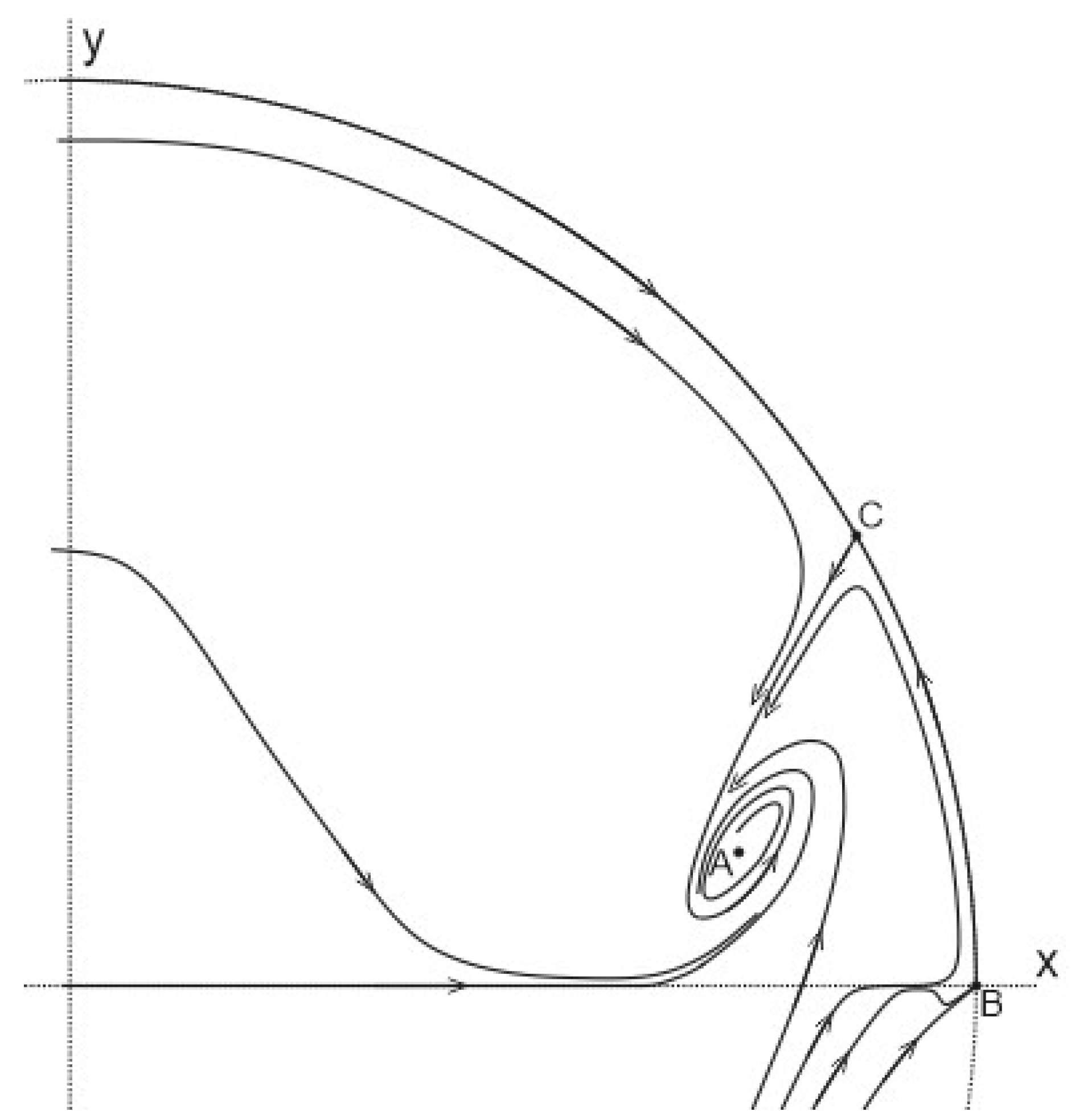
It follows that, with the increasing time the trajectories of the first quadrant tend to the singular point A or to the possible limit cycle surrounding it (Figure 2). □

We now study Hopf bifurcations in system (1). Notice that the right hand side of the second equation in system (1) is not polynomial. First we move the origin to the singular point A. Then we take a power series expansion of the right side of the second equation with three terms, obtaining system

$$\begin{array}{cc}\hfill \dot{x}=& F_1(x,y),\hfill \\ \hfill \dot{y}=& F_2(x,y),\hfill \end{array}$$

(11)

where

$F_1(x,y)=\frac{1}{1-s}x+\frac{1-a+2as-a{s}^2}{s-1}y-xy+y^2$ and

$F_2(x,y)=-\frac{s}{(-1+s)(-a-b+s+2as+3bs-a{s}^2-3b{s}^2+b{s}^3)}x+\frac{1}{(-1+s)}y$

$-\frac{s}{-a-b+s+2as+3bs-a{s}^2-3b{s}^2+b{s}^3}xy+\frac{a+b-3as-3bs+s^2+3a{s}^2+3b{s}^2-a{s}^3-b{s}^3}{s(-a-b+s+2as+3bs-a{s}^2-3b{s}^2+b{s}^3)}{y}^2$

$+\frac{(a+b){(-1+s)}^4}{s^2(-a-b+s+2as+3bs-a{s}^2-3b{s}^2+b{s}^3)}{y}^3.$

The quadratic part of (5) is

$${\mathsf{\Phi }}_2(x,y)=\frac{s}{2(a{(s-1)}^2-b{(s-1)}^3-s)}{x}^2+xy+\frac{-1+a{(s-1)}^2}{2}{y}^2$$

(12)

and it is positive defined for the imposed conditions on the parameters.

The calculations yield that the first Lyapunov quantity of (6) is equal to

$$\begin{array}{ll}{g}_1& =((a+b){(s-1)}^6(a(2s-1)+b(s-1)(1+(s-1)s)))/(s(-a{(s-1)}^2+b{(s-1)}^3+s)\\ & (7b^2{(s-1)}^6+3a^4{(s-1)}^8+16b{(s-1)}^{3}s+12s^2-6a^3{(s-1)}^6(1+b{(s-1)}^3+s)\\ & -2a{(s-1)}^2(3b{(s-1)}^6+7b{(s-1)}^3(1+s)+4s(2+s))+a^2{(s-1)}^4(7+3b^2{(s-1)}^6+\hfill \\ & 6b{(s-1)}^3(2+s)+s(14+3s)))).\hfill \end{array}$$

(13)

Theorem 3.

The system (1) admits a supercritical Hopf bifurcation, but it does not admit a degenerate Hopf bifurcation for the required values of the variables and the parameters.

Proof. 

For system (1) subcritical Hopf bifurcation occurs, as describe in theory above, if first Lypunov quantity is positive. Hence the semialgebraic system must be satisfied

$$g_1\ge 0\wedge s>1\wedge a>\frac{s}{{(s-1)}^2}\wedge b>0\wedge b<\frac{a}{s^2-s},$$

(14)

where $g_1$ is defined as (13). In order for eigenvalues to be purely imaginary the remaining conditions of (14) must be satisfy, see Theorem 1 above.

Using the command Reduce of the computer algebra system MATHEMATICA, we have proven that this system is unsolvable. Thus, the singular point A is a stable focus and the only Hopf bifurcation possible for system (1) is a supercritical Hopf bifurcation. □

Note, the method which can be used to obtained the asymptotic expression on the solution near the Hopf bifurcation is presented in [15].

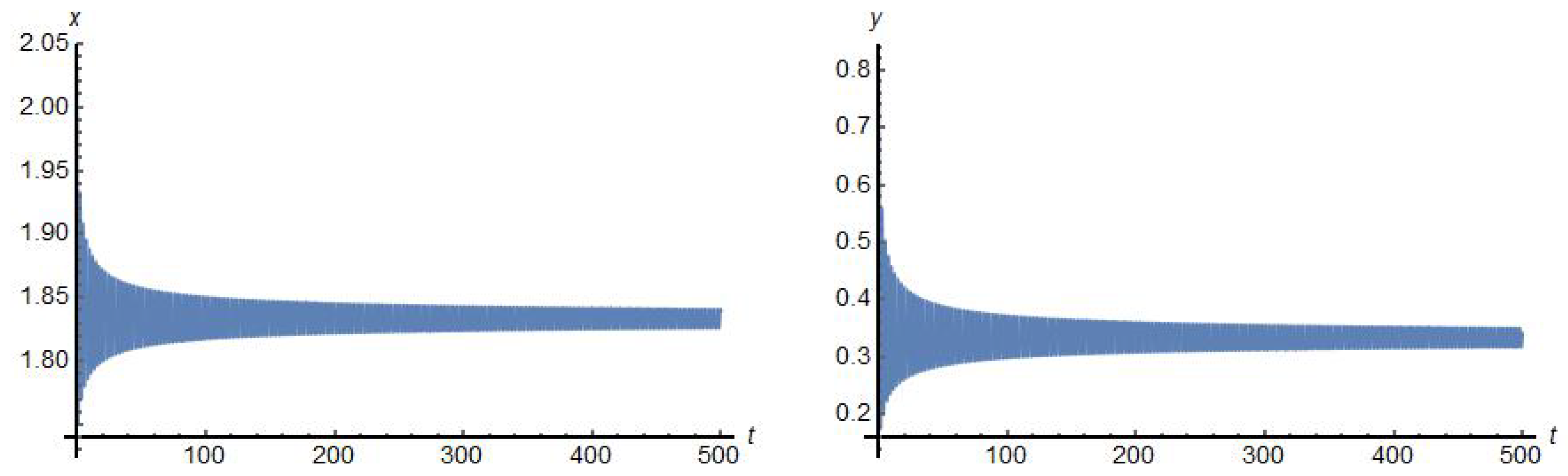
Due to a result from [5], the system (1) admits relaxation oscillations when $b,K\ll 1,c>1$ and $c{b}^{\frac{1}{2}}{(c-1)}^{\frac{1}{2}}<a<c-c^{\frac{1}{2}}$. A suitable set of parameters for Hopf bifurcation is $a=0.5,b=0.01,$$c=2.04,K=0.0575$. With these values of parameters system (1) has a stable focus in the only finite singular point (Figure 3). With perturbation of the parameter $K=0.06$ the singular point becomes an unstable focus and a stable limit cycle around it appears.

According to [5] the parameter c can be chosen from the interval $(1.866,3.2982)$ for the relaxation oscillations still to be preserved. However, the eigenvalues of Jacobian matrix calculated at the singular point have to be imaginary with nonzero imaginary part $\beta$ and positive real part $\alpha$ for the stable limit cycle. They depend on the parameter c in the following manner:

$$\begin{array}{cc}\hfill \alpha \left(c\right)& =5.2+\frac{5.355}{0.51-c}-\frac{2.601}{c}-0.196c,\hfill \\ \hfill \beta \left(c\right)& =\frac{19.6078\sqrt{45.7679-696.813c+3085.61c^2-2532.31c^3+573.521c^4-54.06c^5+c^6}}{c(-51+100c)}\hfill \end{array}$$

(15)

Thus, for the oscillations in general, the parameter c has to be chosen from the interval $I_c=(2.03085,24.8652)$.

Calculations show that the amplitude of the limit cycle depends on the parameter c almost linearly (Figure 4 and Figure 5).

To conclude, we have examined some properties of a two-dimensional system of ordinary differential equations. We focused on the behaviour of the vector field of this system for the positive values of the species and parameters. Some results on this system of a well-stirred isotermal reaction model were known till now, but our approach was different. In [5], one example of the limit cycle oscillations is computed using numerical approach. We extended these results and approached it analytically. Using the theory of Hopf bifurcation we have found the general sufficient conditions on parameters of the system under which a stable limit cycle arises in the phase space of the system. We have described the behaviour of trajectories in the vicinity of the finite singularity in first quadrant and the whole first quadrant. We have used the blow-up method, which is not known in a big extend. Finally, we have shown the correlation between the real part of the eigenvalues of the Jacobian matrix, calculated at the unstable focus inside the limit cycle and the amplitude of the limit cycle on the example. There are still some open problems to be studied connected to system (1). Not regarding on the chemical relations of parameters of system, we can study the global phase portraits. From what we observed in the neighbourhood of the singularity in infinity in first quadrant the behaviour can be very interesting. As seen in Figure 4 the change seems to be linear for our example and it is noticeable the same on Figure 5. Similar dependence was noticed in other examples but the proof for such correlation could be a good topic for further investigation.