Time-Varying Vector Norm and Lower and Upper Bounds on the Solutions of Uniformly Asymptotically Stable Linear Systems

Abstract

Based on the eigenvalue idea and the time-varying weighted vector norm in the state space ${\mathbb{R}}^n$ we construct here the lower and upper bounds of the solutions of uniformly asymptotically stable linear systems. We generalize the known results for the linear time-invariant systems to the linear time-varying ones.

1. Introduction

In addition to the Lyapunov stability criteria for the linear system of ordinary differential equations $\dot{x}=A\left(t\right)x,$ $\dot{x}=dx/dt,$ $t\ge t_0,$ $x\in {\mathbb{R}}^n,$ other types of conditions guaranteeing the stability often are useful. Typically these are sufficient conditions that are proved by application of the Lyapunov stability theorems [1], or the Gronwall–Bellman inequality [2], though sometimes either technique can be used, and sometimes both are used in the same proof of a stability criterion. One of these useful results for stability analysis of the linear systems is the following theorem ([3], p. 132, Theorem 8.2).

Theorem 1.

For the linear system $\dot{x}=A\left(t\right)x,$ $t\ge t_0$ denote the largest and smallest point-wise eigenvalues of $A^T\left(t\right)+A\left(t\right)$ by ${\lambda }_{max}\left(t\right)$ and ${\lambda }_{min}\left(t\right).$ Then for any $t_0$ and $x\left(t_0\right)$ the solution $x\left(t\right)$ satisfies

$${∥x\left(t_0\right)∥}_I{\mathrm{e}}^{1/2\underset{t_0}{\overset{t}{\int }}{\lambda }_{min}\left(\tau \right)d\tau }\le {∥x\left(t\right)∥}_I\le {∥x\left(t_0\right)∥}_I{\mathrm{e}}^{1/2\underset{t_0}{\overset{t}{\int }}{\lambda }_{max}\left(\tau \right)d\tau },t\ge t_0.$$

(1)

Throughout the whole paper it is assumed that a matrix function $A(·):$ $[t_0,\infty )\to {\mathbb{R}}^{n\times n}$ is continuous.

This theorem belongs, as a special case, to the wider family of sufficient conditions for stability of the linear systems based on the “logarithmic measure” of the system matrices ([4], p. 58, Theorem 3) taking into account the fact that for the Euclidean norm ${∥·∥}_I$ the “logarithmic measure” of a real matrix A is just the largest eigenvalue of $\frac{1}{2}(A^T+A)$ ([4], p. 41).

Our aim in this paper is to prove more useful theorem based on the eigenvalues idea for estimating asymptotics of the solutions of uniformly asymptotically stable linear systems. The theory is illustrated by two examples.

Notations, Definitions and Preliminary Results

Let ${\mathbb{R}}^n$ denotes n-dimensional vector space over the real numbers, $x={(x_1,\cdots ,x_n)}^T\in {\mathbb{R}}^n$ is a column vector and the symbol $∥·∥$ refers to any (real) vector norm on ${\mathbb{R}}^n.$ Specifically, for a symmetric, positive definite real matrix $H,$ we define the weight H vector norm ${∥x∥}_H\triangleq {\left(x^{T}Hx\right)}^{1/2}.$ Obviously, for $H=I$ ($I=$ the $n\times n$ identity matrix) we obtain the Euclidean norm, ${∥x∥}_I.$ For the matrices $H\in {\mathbb{R}}^{n\times n}$ as an operator norm we will use an induced norm. Particularly, for weight H vector norm in ${\mathbb{R}}^n,$ the norm ${∥M∥}_H={\left({\lambda }_{max}\left[{\widehat{M}}^T\widehat{M}\right]\right)}^{1/2}$ where $\widehat{M}=H^{1/2}M{H}^{-1/2},$ as was proved in [5]. Further, ${\lambda }_i\left[M\right],$ $i=1,\cdots ,n$ denotes the eigenvalues of the matrix $M,$ ${\lambda }_{min}\left[M\right]=min\{{\lambda }_i\left[M\right]:i=1,\cdots ,n\}$ and, analogously, ${\lambda }_{max}\left[M\right]=max\{{\lambda }_i\left[M\right]:i=1,\cdots ,n\}.$

In this paper we will deal solely with the uniformly asymptotically (⇔ uniformly exponentially) stable linear systems ([1], Theorem 4.11), ([3], Theorem 6.13); for the different types of stability and their relation, see e.g., [6].

Definition 1

([1,3]). The linear system $\dot{x}=A\left(t\right)x$ is called uniformly asymptotically stable (UAS) if there exist finite positive constants $\gamma ,$λ such that for any $t_0$ and $x\left(t_0\right)$ the corresponding solution satisfies

$$∥x\left(t\right)∥\le \gamma ∥x\left(t_0\right)∥{\mathrm{e}}^{-\lambda (t-t_0)},t\ge t_0.$$

We recall that the transition matrix of the linear system $\dot{x}=A\left(t\right)x$ is $\mathsf{\Phi }(t,\tau )\triangleq X\left(t\right)X^{-1}\left(\tau \right),$ where $X\left(t\right),$ $t\ge t_0$ is a fundamental matrix of the system. In particular, if $A\left(t\right)=A$ is an $n\times n$ constant matrix, then the transition matrix is $\mathsf{\Phi }(t,\tau )={\mathrm{e}}^{A(t-\tau )}.$

For the following theorem see, e.g., ([1], p. 156, Theorem 4.11) or ([3], p. 102, Theorem 6.7).

Theorem 2.

The linear system $\dot{x}=A\left(t\right)x$ is uniformly asymptotically stable if and only if there exist finite positive constants $\gamma ,$λ such that

$$∥\mathsf{\Phi }(t,\tau )∥\le \gamma {\mathrm{e}}^{-\lambda (t-\tau )}$$

for all $t,\tau$ such that $t\ge \tau \ge t_0.$

Theorem 1 leads to proof of some simple criterion based on the eigenvalues of $A^T\left(t\right)+A\left(t\right)$ ([3], p. 133, Corollary 8.4); for a wider context in connection with so called “logarithmic measure” of the matrices see also, e.g., [7,8,9].

Corollary 1.

If there exist real positive constants $\tilde{\gamma },$ $\tilde{\lambda }$ such that the largest point-wise eigenvalue of $A^T\left(t\right)+A\left(t\right)$ satisfies

$$\underset{\tau }{\overset{t}{\int }}{\lambda }_{max}\left[A^T\left(s\right)+A\left(s\right)\right]ds\le \tilde{\gamma }-\tilde{\lambda }(t-\tau )$$

(2)

for all $t,\tau$ such that $t\ge \tau \ge t_0,$ then the linear system $\dot{x}=A\left(t\right)x$ is UAS.

This criterion is quite conservative in the sense that many UAS linear systems do not satisfy the condition (2) as demonstrated by the following example.

Example 1.

The system $\dot{x}=Ax,$ $t\ge 0$ with

$$A=\left(\begin{array}{cc}0& \sqrt{10}\\ -\sqrt{10}& -2\end{array}\right)$$

is UAS because ${\lambda }_{1,2}\left[A\right]=-1\pm 3\mathrm{i}.$ Because ${\lambda }_{max}[A^T+A]=0,$ there does not exist a pair of positive constants $\tilde{\gamma },$ $\tilde{\lambda }$ such that the inequality (2) holds for all $t\ge \tau \ge 0,$ and so Corollary 1 is not applicable in this particular case. A straightforward computation by Theorem 1 gives

$${∥x\left(0\right)∥}_I{\mathrm{e}}^{-2t}\le {∥x\left(t\right)∥}_I\le {∥x\left(0\right)∥}_I$$

for all $t\ge 0.$

Despite such examples the eigenvalue idea is not to be completely rejected. In Theorem 3 below we prove for the UAS linear systems $\dot{x}=A\left(t\right)x$ the stronger result, generalizing Theorem 1 in such a way as to be meaningfully applicable to every UAS system.

2. Main Results

The main results of this paper are summarized in the following theorem generalizing ([5], Theorem 3.1) to the linear time-varying systems. Recall that although its claims are mainly of theoretical relevance, providing the necessary conditions for exponential stability, within its framework without giving details and exact mathematical explanation the important results regarding convergent systems were derived in [10]; for the definitions and comparisons with the notion of incremental stability see also [11]. Moreover, this theorem provides also the lower bound on the solutions generally classified as difficult to obtain.

Theorem 3.

If the linear system $\dot{x}=A\left(t\right)x,$ is UAS, where $A(·):$ $[t_0,\infty ]\to {\mathbb{R}}^{n\times n}$ is a continuous matrix function, then there exists a continuous, symmetric and positive definite matrix function $H(·):$ $[t_0,\infty ]\to {\mathbb{R}}^{n\times n}$ such that every solution $x\left(t\right)$ of the system satisfies

$${\left(\frac{{\lambda }_{min}\left[H\left(t\right)\right]}{{\lambda }_{max}\left[H\left(t\right)\right]}\right)}^{1/2}{∥x\left(t_0\right)∥}_I{\mathrm{e}}^{-\frac{1}{2}\underset{t_0}{\overset{t}{\int }}\frac{d\tau }{{\lambda }_{min}\left[H\left(\tau \right)\right]}}\le {∥x\left(t\right)∥}_I$$

$$\le {\left(\frac{{\lambda }_{max}\left[H\left(t\right)\right]}{{\lambda }_{min}\left[H\left(t\right)\right]}\right)}^{1/2}{∥x\left(t_0\right)∥}_I{\mathrm{e}}^{-\frac{1}{2}\underset{t_0}{\overset{t}{\int }}\frac{d\tau }{{\lambda }_{max}\left[H\left(\tau \right)\right]}}\mathrm{for}\mathrm{all}t\ge t_0,$$

(3)

and there exist two positive real constant $\gamma ,\lambda$ such that

$${\lambda }_{max}\left[H\left(t\right)\right]\le \frac{{\gamma }^2}{2\lambda }.$$

In particular, if $A\left(t\right)$ is bounded, ${∥A\left(t\right)∥}_I\le L$ for all $t\ge t_0$, then

$$\frac{1}{2L}\le {\lambda }_{min}\left[H\left(t\right)\right]\le {\lambda }_{max}\left[H\left(t\right)\right]\le \frac{{\gamma }^2}{2\lambda }.$$

(4)

Proof. 

Set

$$H\left(t\right)=\underset{t}{\overset{\infty }{\int }}{\mathsf{\Phi }}^T(\tau ,t)\mathsf{\Phi }(\tau ,t)d\tau ,t\ge t_0.$$

In particular, if $A\left(t\right)=A$ is a constant matrix, we have

$$H=\underset{0}{\overset{\infty }{\int }}{\mathrm{e}}^{A^T\tau }{\mathrm{e}}^{A\tau }d\tau .$$

We begin with the analysis of the properties of the matrix function $H(·).$ Observe that $H\left(t\right)$ is symmetric and positive definite because such is the integrand ${\mathsf{\Phi }}^T(\tau ,t)\mathsf{\Phi }(\tau ,t)$ ([12], Corollary 14.2.10). The use of

• The Rayleigh–Ritz ratio [13],
• The fact that ${∥\mathsf{\Phi }(\tau ,t)∥}_I={∥{\mathsf{\Phi }}^T(\tau ,t)∥}_I$ because every matrix and its transpose have the same characteristic polynomial ([12], Lemma 21.1.2),
• The fact that spectral radius of the matrix ${\mathsf{\Phi }}^T(\tau ,t)\mathsf{\Phi }(\tau ,t)$ is less or equal to any induced matrix norm $∥{\mathsf{\Phi }}^T(\tau ,t)\mathsf{\Phi }(\tau ,t)∥,$ and
• Theorem 2

yields for every fixed $t\ge t_0$ and $x\in {\mathbb{R}}^n$ that

$$x^{T}H\left(t\right)x\le {\lambda }_{max}\left[\underset{t}{\overset{\infty }{\int }}{\mathsf{\Phi }}^T(\tau ,t)\mathsf{\Phi }(\tau ,t)d\tau \right]{∥x∥}_I^2\le {∥\underset{t}{\overset{\infty }{\int }}{\mathsf{\Phi }}^T(\tau ,t)\mathsf{\Phi }(\tau ,t)d\tau ∥}_I{∥x∥}_I^2$$

$$\le {∥x∥}_I^2\underset{t}{\overset{\infty }{\int }}{∥\mathsf{\Phi }(\tau ,t)∥}_I^{2}d\tau \le {∥x∥}_I^2\underset{t}{\overset{\infty }{\int }}{\gamma }^2{\mathrm{e}}^{-2\lambda (\tau -t)}d\tau =\frac{{\gamma }^2}{2\lambda }{∥x∥}_I^2,$$

where $\gamma ,$ $\lambda$ are the constants given by Theorem 2. As a consequence, ${\lambda }_{max}\left[H\left(t\right)\right]\le \frac{{\gamma }^2}{2\lambda }$ because there is equality $x^{T}H\left(t\right)x={\lambda }_{max}\left[H\left(t\right)\right]{∥x∥}_I^2$ for x equal to the eigenvector corresponding to ${\lambda }_{max}\left[H\left(t\right)\right].$ To prove the left inequality in (4) we will need the following result.

Lemma 1.

If ${∥A\left(t\right)∥}_I\le L$ for all $t\ge t_0,$ then the solution $x\left(t\right)$ of the $\dot{x}=A\left(t\right)x$ satisfies

$${∥x\left(t_0\right)∥}_I{\mathrm{e}}^{-L(t-t_0)}\le {∥x\left(t\right)∥}_I\le {∥x\left(t_0\right)∥}_I{\mathrm{e}}^{L(t-t_0)},t\ge t_0.$$

(5)

Observe that the right-hand side inequality is uninteresting for UAS systems, every estimate of ${∥x\left(t\right)∥}_I$ would grow exponentially as $t\to \infty .$

Proof. 

The claim of the lemma follows immediately from the chain of inequalities

$${\lambda }_{max}\left[A^T\left(t\right)+A\left(t\right)\right]\le {∥A^T\left(t\right)+A\left(t\right)∥}_I\le 2{∥A\left(t\right)∥}_I\le 2L,$$

$${\lambda }_{min}\left[A^T\left(t\right)+A\left(t\right)\right]\ge -{∥A^T\left(t\right)+A\left(t\right)∥}_I\ge -2{∥A\left(t\right)∥}_I\ge -2L,$$

and (1). □

Now if $\varphi \left(\tau \right)$ is a solution of $d\varphi /d\tau =A\left(\tau \right)\varphi$ starting at $(t,x),$ that is, $\varphi \left(\tau \right)=\mathsf{\Phi }(\tau ,t)x,$ then for all $x\in {\mathbb{R}}^n$ one gets

$$x^{T}H\left(t\right)x=x^T\left(\underset{t}{\overset{\infty }{\int }}{\mathsf{\Phi }}^T(\tau ,t)\mathsf{\Phi }(\tau ,t)d\tau \right)x=\underset{t}{\overset{\infty }{\int }}{\varphi }^T\left(\tau \right)\varphi \left(\tau \right)d\tau$$

and, by (5),

$$\underset{t}{\overset{\infty }{\int }}{∥\varphi \left(\tau \right)∥}_I^{2}d\tau \ge {∥x∥}_I^2\underset{t}{\overset{\infty }{\int }}{\mathrm{e}}^{-2L(\tau -t)}d\tau =\frac{1}{2L}{∥x∥}_I^2.$$

Arguing analogously as above, ${\lambda }_{min}\left[H\left(t\right)\right]\ge \frac{1}{2L}$ and the inequality (4) is proved.

Now we are ready to prove the remaining part of the theorem, namely the inequality (3). Suppose $x\left(t\right)$ is a solution of $\dot{x}=A\left(t\right)x$ corresponding to a given $t_0$ and nonzero $x\left(t_0\right).$ Let us formally consider a time-varying weighted vector norm of the solutions ${∥x\left(t\right)∥}_{H\left(t\right)}.$ Then

$$\frac{d}{dt}{∥x\left(t\right)∥}_{H\left(t\right)}^2=\frac{d}{dt}\left[x^T\left(t\right)H\left(t\right)x\left(t\right)\right]=x^T\left(t\right)\left[A^T\left(t\right)H\left(t\right)+\dot{H}\left(t\right)+H\left(t\right)A\left(t\right)\right]x\left(t\right).$$

(6)

Now we show that the function $H\left(t\right)$ satisfies time-varying Lyapunov equation (e.g., [1,3,14])

$$\dot{H}\left(t\right)+A^T\left(t\right)H\left(t\right)+H\left(t\right)A\left(t\right)=-I.$$

Using the Equations ([15], p. 70) and ([3], p. 62)

$$\frac{d}{dt}\mathsf{\Phi }(\tau ,t)=-\mathsf{\Phi }(\tau ,t)A\left(t\right),$$

$$\frac{d}{dt}{\mathsf{\Phi }}^T(\tau ,t)=-A^T\left(t\right){\mathsf{\Phi }}^T(\tau ,t)$$

and

$$\mathsf{\Phi }(\tau =\infty ,t)=0(\Leftarrow \mathrm{UAS}),\mathsf{\Phi }(t,t)=I,$$

we obtain that

$$\dot{H}\left(t\right)=\underset{t}{\overset{\infty }{\int }}{\mathsf{\Phi }}^T(\tau ,t)\left[\frac{\partial }{\partial t}\mathsf{\Phi }(\tau ,t)\right]d\tau +\underset{t}{\overset{\infty }{\int }}\left[\frac{\partial }{\partial t}{\mathsf{\Phi }}^T(\tau ,t)\right]\mathsf{\Phi }(\tau ,t)d\tau -I$$

$$=-\underset{t}{\overset{\infty }{\int }}{\mathsf{\Phi }}^T(\tau ,t)\mathsf{\Phi }(\tau ,t)d\tau A\left(t\right)-A^T\left(t\right)\underset{t}{\overset{\infty }{\int }}{\mathsf{\Phi }}^T(\tau ,t)\mathsf{\Phi }(\tau ,t)d\tau -I$$

$$=-A^T\left(t\right)H\left(t\right)-H\left(t\right)A\left(t\right)-I.$$

Returning to (6), $\frac{d}{dt}{∥x\left(t\right)∥}_{H\left(t\right)}^2=-{∥x\left(t\right)∥}_I^2.$ Dividing through by ${∥x\left(t\right)∥}_{H\left(t\right)}^2$ which is positive at each $t\ge t_0,$ the Rayleigh–Ritz ratio yields

$$-\frac{1}{{\lambda }_{min}\left[H\left(t\right)\right]}\le \frac{\frac{d}{dt}{∥x\left(t\right)∥}_{H\left(t\right)}^2}{{∥x\left(t\right)∥}_{H\left(t\right)}^2}=-\frac{{∥x∥}_I^2}{x^{T}H\left(t\right)x}\le -\frac{1}{{\lambda }_{max}\left[H\left(t\right)\right]}.$$

Integrating from $t_0$ to any $t\ge t_0$ one gets

$$-\underset{t_0}{\overset{t}{\int }}\frac{d\tau }{{\lambda }_{min}\left[H\left(\tau \right)\right]}\le \ln {∥x\left(t\right)∥}_{H\left(t\right)}^2-\ln {∥x\left(t_0\right)∥}_{H\left(t\right)}^2\le -\underset{t_0}{\overset{t}{\int }}\frac{d\tau }{{\lambda }_{max}\left[H\left(\tau \right)\right]}.$$

Exponentiation followed by taking the nonnegative square root gives for all $t\ge t_0$ the inequality

$${∥x\left(t_0\right)∥}_{H\left(t\right)}{\mathrm{e}}^{-\frac{1}{2}\underset{t_0}{\overset{t}{\int }}\frac{d\tau }{{\lambda }_{min}\left[H\left(\tau \right)\right]}}\le {∥x\left(t\right)∥}_{H\left(t\right)}\le {∥x\left(t_0\right)∥}_{H\left(t\right)}{\mathrm{e}}^{-\frac{1}{2}\underset{t_0}{\overset{t}{\int }}\frac{d\tau }{{\lambda }_{max}\left[H\left(\tau \right)\right]}}.$$

(7)

Finally using “norm conversion rule” between different weight $H_1$ and $H_2$ (recall $H_1,$ $H_2$ are symmetric and positive definite matrices)

$$\frac{{\lambda }_{min}\left[H_1\right]}{{\lambda }_{max}\left[H_2\right]}\le \frac{{∥x∥}_{H_1}^2}{{∥x∥}_{H_2}^2}=\frac{x^T{H}_{1}x}{x^T{H}_{2}x}\le \frac{{\lambda }_{max}\left[H_1\right]}{{\lambda }_{min}\left[H_2\right]}\mathrm{for}x\ne 0,$$

we obtain the inequality (3). □

Remark 1.

Combining ([5], Lemma 2.3, Theorem 2.1) and ([4], p. 58, Theorem 3) we obtain

$${∥x\left(t_0\right)∥}_{\tilde{H}}{\mathrm{e}}^{-\underset{t_0}{\overset{t}{\int }}\frac{d\tau }{{\lambda }_{min}\left[\tilde{H}\right]}}\le {∥x\left(t\right)∥}_{\tilde{H}}\le {∥x\left(t_0\right)∥}_{\tilde{H}}{\mathrm{e}}^{-\underset{t_0}{\overset{t}{\int }}\frac{d\tau }{{\lambda }_{max}\left[\tilde{H}\right]}}$$

which is a special case of (7) if $H\left(t\right)=\tilde{H}/2.$ Observe that $\tilde{H}$ in [5] satisfies the Lyapunov equation $A^T\tilde{H}+A\tilde{H}=-2I.$ Thus, Theorem 3 represents generalization to the time-varying systems. Moreover, because $x\left(t\right)=\mathsf{\Phi }(t,t_0)x\left(t_0\right),$ and from the properties of induced matrix norm we have

$${\left(\frac{{\lambda }_{min}\left[H\left(t\right)\right]}{{\lambda }_{max}\left[H\left(t\right)\right]}\right)}^{1/2}{\mathrm{e}}^{-\frac{1}{2}\underset{t_0}{\overset{t}{\int }}\frac{d\tau }{{\lambda }_{min}\left[H\left(\tau \right)\right]}}\le {∥\mathsf{\Phi }(t,t_0)∥}_I\le {\left(\frac{{\lambda }_{max}\left[H\left(t\right)\right]}{{\lambda }_{min}\left[H\left(t\right)\right]}\right)}^{1/2}{\mathrm{e}}^{-\frac{1}{2}\underset{t_0}{\overset{t}{\int }}\frac{d\tau }{{\lambda }_{max}\left[H\left(\tau \right)\right]}}$$

for $t\ge \tau \ge t_0.$ The general idea of the proof follows, e.g., the proof of ([3], p. 100, Theorem 6.4) and so the proof is omitted here. The last inequality generalizes ([5], Theorem 3.1) to the linear time-varying systems. Moreover, we get also the lower bound on the solutions.

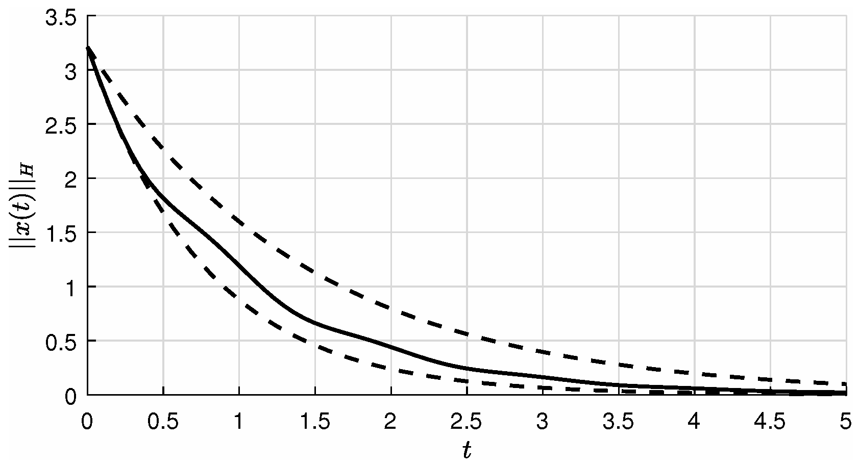
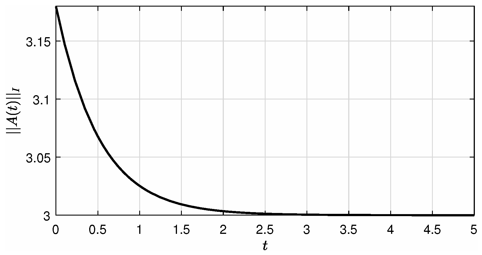
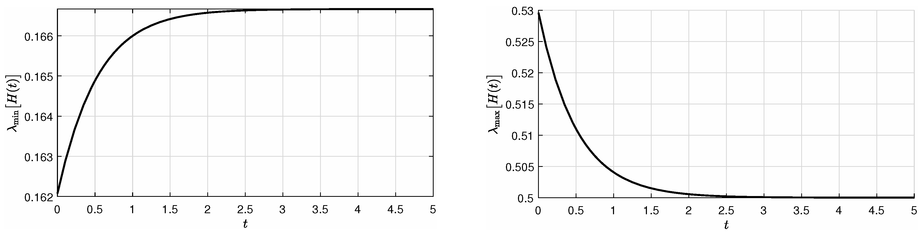
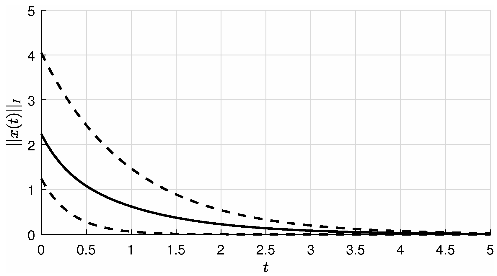
3. Simulation Results

Example 2 (Example 1 revisited).

Let us consider again the system from Example 1. One gets

$${\mathrm{e}}^{At}=\frac{{\mathrm{e}}^{-t}}{3}\left(\begin{array}{cc}3cos3t+sin3t& \sqrt{10}sin3t\\ -\sqrt{10}sin3t& 3cos3t-sin3t\end{array}\right)$$

and

$$H=\underset{0}{\overset{\infty }{\int }}{\mathrm{e}}^{A^T\tau }{\mathrm{e}}^{A\tau }d\tau =\left(\begin{array}{cc}3/5& \sqrt{10}/20\\ \sqrt{10}/20& 1/2\end{array}\right).$$

Since the eigenvalues of H are ${\lambda }_{min}\left[H\right]=11/20-\sqrt{11}/20,$ ${\lambda }_{max}\left[H\right]=11/20+\sqrt{11}/20,$ the inequality (7) for $t_0=0$ becomes

$${∥x\left(0\right)∥}_H{\mathrm{e}}^{-\frac{10t}{11-\sqrt{11}}}\le {∥x\left(t\right)∥}_H\le {∥x\left(0\right)∥}_H{\mathrm{e}}^{-\frac{10t}{11+\sqrt{11}}},$$

(8)

where ${∥x∥}_H={\left(3x_1^2/5+\left(\sqrt{10}/10\right)x_1{x}_2+x_2^2/2\right)}^{1/2}.$ The result of simulation in the Matlab environment demonstrating effectiveness of the developed approach is depicted in Figure 1.

Figure 1. Solution of the linear time-invariant system from Example 1 and 2 with an initial state$x\left(0\right)={(x_1\left(0\right),x_2\left(0\right))}^T={(-4,3)}^T$(the solid line) and the lower and upper bound given by (8) (the dashed lines).

Example 3.

For the linear time-varying system $\dot{x}=A\left(t\right)x,$ $t\ge 0$ with

$$A\left(t\right)=\left(\begin{array}{cc}-1& {\mathrm{e}}^{-t}\\ 0& -3\end{array}\right)$$

the fundamental matrix of the system (see [6]) is

$$X\left(t\right)=\left(\begin{array}{cc}{\mathrm{e}}^{-t}& \frac{{\mathrm{e}}^{-t}}{3}-\frac{{\mathrm{e}}^{-4t}}{3}\\ 0& {\mathrm{e}}^{-3t}\end{array}\right).$$

The eigenvalues of $A^T\left(t\right)A\left(t\right),t\ge 0$ satisfy

$${\lambda }_1\left[A^T\left(t\right)A\left(t\right)\right]=\frac{{\mathrm{e}}^{-2t}}{2}-\frac{{\mathrm{e}}^{-2t}}{2}{\left[\left(4{\mathrm{e}}^{2t}+1\right)\left(16{\mathrm{e}}^{2t}+1\right)\right]}^{1/2}+5\to 1$$

as $t\to \infty ,$

$${\lambda }_2\left[A^T\left(t\right)A\left(t\right)\right]=\frac{{\mathrm{e}}^{-2t}}{2}+\frac{{\mathrm{e}}^{-2t}}{2}{\left[\left(4{\mathrm{e}}^{2t}+1\right)\left(16{\mathrm{e}}^{2t}+1\right)\right]}^{1/2}+5\to 9$$

as $t\to \infty ;$ ${\lambda }_1\left[A^T\left(t\right)A\left(t\right)\right]<{\lambda }_2\left[A^T\left(t\right)A\left(t\right)\right]$ for all $t\ge 0$ and ${∥A\left(0\right)∥}_I=3.1796,$ ${∥A\left(t\right)∥}_I={\left({\lambda }_{max}\left[A^T\left(t\right)A\left(t\right)\right]\right)}^{1/2}\to 3$ (monotonically) as $t\to \infty$ and therefore the constant L in (4) is equal to ${∥A\left(0\right)∥}_I=3.1796$ (Figure 2).

Figure 2. Time development of the${∥A\left(t\right)∥}_I,$$t\ge 0$.

The transition matrix is

$$\mathsf{\Phi }(t,\tau )=X\left(t\right)X^{-1}\left(\tau \right)=\left(\begin{array}{cc}{\mathrm{e}}^{\tau -t}& \frac{{\mathrm{e}}^{-t}}{3}-\frac{{\mathrm{e}}^{3\tau -4t}}{3}\\ 0& {\mathrm{e}}^{3\tau -3t}\end{array}\right)$$

and the matrix function $H\left(t\right)$ from Theorem 3 is

$$H\left(t\right)=\underset{t}{\overset{\infty }{\int }}{\mathsf{\Phi }}^T(\tau ,t)\mathsf{\Phi }(\tau ,t)d\tau =\left(\begin{array}{cc}\frac{1}{2}& \frac{{\mathrm{e}}^{-t}}{10}\\ \frac{{\mathrm{e}}^{-t}}{10}& \frac{{\mathrm{e}}^{-2t}}{40}+\frac{1}{6}\end{array}\right)$$

with the eigenvalues

$${\lambda }_{min}\left[H\left(t\right)\right]=\frac{{\mathrm{e}}^{-2t}}{80}-\frac{{\mathrm{e}}^{-2t}}{240}{\left[336{\mathrm{e}}^{2t}+1600{\mathrm{e}}^{4t}+9\right]}^{1/2}+\frac{1}{3}\to 1/6$$

(9)

$${\lambda }_{max}\left[H\left(t\right)\right]=\frac{{\mathrm{e}}^{-2t}}{80}+\frac{{\mathrm{e}}^{-2t}}{240}{\left[336{\mathrm{e}}^{2t}+1600{\mathrm{e}}^{4t}+9\right]}^{1/2}+\frac{1}{3}\to 1/2$$

(10)

as $t\to \infty$ (Figure 3).

Figure 3. Time development of the functions${\lambda }_{min}\left(H\left(t\right)\right)$and${\lambda }_{max}\left(H\left(t\right)\right),$$t\ge 0$.

The integrals in (3) can be calculated explicitly

$$-\frac{1}{2}\underset{0}{\overset{t}{\int }}\frac{d\tau }{{\lambda }_{min}\left[H\left(\tau \right)\right]}=\frac{3}{2}\ln \left(\rho -1\right)-\frac{5}{2}\ln \left(\frac{2\sqrt{6}}{5}-\rho +\frac{7}{5}\right)$$

$$+\frac{1}{2}\ln \left(\left(\rho +1\right)\left(2\sqrt{6}-\rho +5\right)\right)+3.2375954052$$

and

$$-\frac{1}{2}\underset{0}{\overset{t}{\int }}\frac{d\tau }{{\lambda }_{max}\left[H\left(\tau \right)\right]}=\frac{3}{2}\ln \left(\rho +1\right)-\frac{5}{2}\ln \left(\frac{2\sqrt{6}}{5}+\rho +\frac{7}{5}\right)$$

$$+\frac{1}{2}\ln \left(\left(\rho -1\right)\left(2\sqrt{6}+\rho +5\right)\right)+2.1447615497,$$

where

$$\rho ={\left(\frac{100{\mathrm{e}}^{2t}+3\sqrt{6}+\frac{21}{2}}{100{\mathrm{e}}^{2t}-3\sqrt{6}+\frac{21}{2}}\right)}^{1/2}.$$

The result of simulation—the solution of system and the lower and upper bounds—are depicted in the Figure 4.

Figure 4. Solution of the linear time-varying system from Example 3 with initial state$x\left(0\right)={(2,-1)}^T$(the solid line) and the lower and upper bounds given by (3), (9) and (10) (the dashed lines).

Analyzing the properties of matrix function $H\left(t\right)$ it is obvious that

$${\lambda }_{min}\left[H\left(0\right)\right]=\frac{1}{80}-\frac{\sqrt{1945}}{240}+\frac{1}{3}(\approx 0.1621)\le {\lambda }_{min}\left[H\left(t\right)\right],$$

$${\lambda }_{max}\left[H\left(t\right)\right]\le {\lambda }_{max}\left[H\left(0\right)\right]=\frac{1}{80}+\frac{\sqrt{1945}}{240}+\frac{1}{3}(\approx 0.5296)$$

and

$$(-t/2){\left({\lambda }_{min}\left[H\left(0\right)\right]\right)}^{-1}=-3.0845t\le -\frac{1}{2}\underset{0}{\overset{t}{\int }}1/{\lambda }_{min}\left[H\left(\tau \right)\right]d\tau ,$$

$$(-t/2){\left({\lambda }_{max}\left[H\left(0\right)\right]\right)}^{-1}=-0.9441t\ge -\frac{1}{2}\underset{0}{\overset{t}{\int }}1/{\lambda }_{max}\left[H\left(\tau \right)\right]d\tau$$

for every $t\ge 0.$ Thus we obtain more readable approximate estimate of the solutions

$$0.5531{∥x\left(0\right)∥}_I{\mathrm{e}}^{-3.0845t}\le {∥x\left(t\right)∥}_I\le 1.8075{∥x\left(0\right)∥}_I{\mathrm{e}}^{-0.9441t}$$

and Theorem 2 is satisfied for

$$\gamma ={\left(\frac{{\lambda }_{max}\left[H\left(0\right)\right]}{{\lambda }_{min}\left[H\left(0\right)\right]}\right)}^{1/2}={\left(\frac{0.5296}{0.1621}\right)}^{1/2}=1.8075,$$

and

$$\lambda =(1/2){\left({\lambda }_{max}\left[H\left(0\right)\right]\right)}^{-1}=0.9441.$$

4. Conclusions

In this paper we established the lower and upper bounds of all solutions to uniformly asymptotically stable linear time-varying systems from the knowledge of one fundamental matrix solution. Our approach is based on the eigenvalue idea and a time-varying metric on the state space ${\mathbb{R}}^n.$ The simulation experiments demonstrates the effectiveness of the proposed method for estimating solutions, generally classified as “difficult to obtain”, especially in the case of the lower bounds.

References

- Khalil, H.K. Nonlinear Systems, 3rd ed.; Prentice-Hall: Englewood Cliffs, NJ, USA, 2002. [Google Scholar]
- Chicone, C. Ordinary Differential Equations with Applications; (Texts in Applied Mathematics); Springer: New York, NY, USA, 1999; Volume 34. [Google Scholar]
- Rugh, W.J. Linear System Theory, 2nd ed.; Prentice-Hall, Inc.: Upper Saddle River, NJ, USA, 1996. [Google Scholar]
- Coppel, W.A. Stability and Asymptotic Behavior of Differential Equations; D. C. Heath and Company: Boston, MA, USA, 1965. [Google Scholar]
- Hu, G.-D.; Liu, M. The weighted logarithmic matrix norm and bounds of the matrix exponential. Linear Algebra Appl. 2004, 390, 145–154. [Google Scholar] [CrossRef]
- Zhou, B. On asymptotic stability of linear time-varying systems. Automatica 2016, 68, 266–276. [Google Scholar] [CrossRef]
- Afanas’ev, V.N.; Kolmanovskii, V.B.; Nosov, V.R. Mathematical Theory of Control Systems Design; Originally published by Kluwer Academic Publishers in 1996; Springer Science+Business Media: Dordrecht, The Netherlands, 1996. [Google Scholar]
- Dekker, K.; Verwer, J.G. Stability of Runge-Kutta Methods for Stiff Nonlinear Differential Equations; North-Holland: Amsterdam, The Netherlands, 1984. [Google Scholar]
- Desoer, C.A.; Haneda, H. The Measure of a Matrix as a Tool to Analyze Computer Algorithms for Circuit Analysis. IEEE Trans. Circuits Theory 1972, 19, 480–486. [Google Scholar] [CrossRef]
- Lohmiller, W.; Slotine, J.-J.E. On contraction analysis for non-linear systems. Automatica 1998, 34, 683–696. [Google Scholar] [CrossRef]
- Rüffer, B.S.; van de Wouw, N.; Mueller, M. Convergent systems vs. incremental stability. Syst. Control Lett. 2013, 62, 277–285. [Google Scholar]
- Harville, D.A. Matrix Algebra From a Statistician’s Perspective; Springer: New York, NY, USA, 2008. [Google Scholar]
- Horn, R.A.; Johnson, C.R. Matrix Analysis; Cambridge University Press: Cambridge, UK, 1990. [Google Scholar]
- Goh, B.S. Global stability in many-species systems. Am. Nat. 1977, 111, 135–143. [Google Scholar] [CrossRef]
- Coddington, E.A.; Levinson, N. Theory of Ordinary Differential Equations; McGraw-Hill: New York, NY, USA, 1955. [Google Scholar]
© 2020 by the author. Licensee MDPI, Basel, Switzerland. This article is an open access article distributed under the terms and conditions of the Creative Commons Attribution (CC BY) license (http://creativecommons.org/licenses/by/4.0/).