The Triads Geometric Consistency Index in AHP-Pairwise Comparison Matrices

Abstract

The paper presents the Triads Geometric Consistency Index ($T\text{-}GCI$), a measure for evaluating the inconsistency of the pairwise comparison matrices employed in the Analytic Hierarchy Process (AHP). Based on the Saaty’s definition of consistency for AHP, the new measure works directly with triads of the initial judgements, without having to previously calculate the priority vector, and therefore is valid for any prioritisation procedure used in AHP. The $T\text{-}GCI$ is an intuitive indicator defined as the average of the log quadratic deviations from the unit of the intensities of all the cycles of length three. Its value coincides with that of the Geometric Consistency Index ($GCI$) and this allows the utilisation of the inconsistency thresholds as well as the properties of the $GCI$ when using the $T\text{-}GCI$. In addition, the decision tools developed for the $GCI$ can be used when working with triads ($T\text{-}GCI$), especially the procedure for improving the inconsistency and the consistency stability intervals of the judgements used in group decision making. The paper further includes a study of the computational complexity of both measures ($T\text{-}GCI$ and $GCI$) which allows selecting the most appropriate expression, depending on the size of the matrix. Finally, it is proved that the generalisation of the proposed measure to cycles of any length coincides with the $T\text{-}GCI$. It is not therefore necessary to consider cycles of length greater than three, as they are more complex to obtain and the calculation of their associated measure is more difficult.

1. Introduction

Since the origin of the species, humans have used pairwise comparisons to choose between tangible elements. This has generally involved taking the lesser element as a reference unit, and then indicating how many times the greater element “includes” or “dominates” the lesser. This intuitive method for comparing elements has been formalised in the course of human history. After the seminal work of the Majorcan Ramon Llull (1232–1315) (see [1]), the comparisons technique was formally introduced in the second half of the 19th century [2] and further developed in the early years of the 20th century [3]. Following the substantive rationality that was prevalent in the traditional scientific method, pairwise comparisons were generally utilised to order tangible elements, based on an objective attribute with a known unit of reference or measurement scale.

In the mid-1970s, Thomas L. Saaty [4] instigated and refined a new school of thought in the field of multicriteria decisions—the Analytic Hierarchy Process (AHP). Using a hierarchical model of the problem and pairwise comparison to incorporate the preferences of the decision maker, AHP allows for the integration of the objective aspects associated with the traditional scientific method and the subjective aspects associated with the human factor.

The AHP methodology comprises four stages [5]: (i) modelling, or the construction of a hierarchical model; (ii) valuation, or the incorporation of the preferences by means of pairwise comparisons; (iii) prioritisation, or the calculation of the local priorities associated with the nodes of the hierarchy, by means of an existing prioritisation procedure, and the calculation of the global priorities by means of the principle of hierarchical composition; and (iv) synthesis, or the determination of the total priorities of the alternatives by means of one of the available aggregation procedures.

In addition to integrating the subjective with the objective, AHP permits the explicit evaluation of the consistency of the decision maker at the time of eliciting their judgements, whilst admitting small levels of inconsistency. An earlier analysis of inconsistency can be found in [6,7,8].

Given a pairwise comparison matrix $A_{(n\times n)}=\left(a_{ij}\right)$ with $a_{ij}{a}_{ji}=1$ and $a_{ij}>0$, Saaty [4] established that the matrix A is consistent when $a_{ij}{a}_{jk}=a_{ik}\forall i,j,k=1,\dots ,n$. In the same way [9], A is consistent if all the cycles of length three fulfil $a_{ij}{a}_{jk}{a}_{ki}=1\forall i,j,k=1,\dots ,n$.

Although consistency in AHP is defined in terms of triads of the elements of the matrix $A=\left(a_{ij}\right)$, its evaluation, following Saaty’s proposal (and the majority of methods that are traditionally followed for the evaluation of inconsistency), depends on the prioritisation procedure that is employed, that is to say, the measurement of inconsistency is linked to the prioritisation procedure.

Nevertheless, a group of measures explicitly based on the Saaty’s definition of consistency that are not linked to any prioritisation method are being considered. The present work puts forward an inconsistency measure—the Triads Geometric Consistency Index ($T\text{-}GCI$)—which belongs to this last group but that coincides with the Geometric Consistency Index ($GCI$), a measure of the former group. This fact provides a link between both groups of inconsistency measures.

The most relevant contributions of this work are: (i) the definition of the $T\text{-}GCI$; (ii) the demonstration of its relationship with one of the inconsistency measures most used in AHP, the $GCI$ [10], making it possible to use the properties of the $GCI$ as well as its thresholds to make the $T\text{-}GCI$ operative; (iii) the study of the computational complexity of the $T\text{-}GCI$, comparing with that of the $GCI$; and (iv) the generalisation of the $T\text{-}GCI$ to cycles of any length.

After this brief Introduction, the remainder of the article is structured as follows. Section 2 offers a summary of the concept of consistency in AHP and details some measurements for its evaluation that have been used in the scientific literature. Section 3 defines the $T\text{-}GCI$, proves its relationship with the $GCI$, explains its operational behaviour, gives thresholds for evaluation of inconsistency in AHP and analyses its computational complexity. Section 4 places the $T\text{-}GCI$ in a more general context of inconsistency measurements based on cycles of any length and demonstrates that they are coincident with the $T\text{-}GCI$. Section 5 highlights the most important conclusions of the work and suggests some future lines of research.

2. Consistency in the Analytic Hierarchy Process

Defined as the cardinal transitivity in judgements ($a_{ij}{a}_{jk}=a_{ik}\forall i,j,k$), consistency in AHP is a desirable property that reflects a certain rationality, logic or formal coherence in the actions of individuals, especially when they compare intangible aspects for which appropriate measurement scales are not currently available.

Some of the factors that may cause inconsistency are: (i) the ambiguity and complexity of the problem; (ii) the knowledge of the actors in the matter under consideration; (iii) the affective aspects (mood, emotions, personality features, attitudes and motivations) that condition the behaviour of the actors; (iv) the level of attention (errors in the response) during the assessment process [11,12]; and (v) the rationality of the procedure followed when incorporating preferences, especially when working with subjective aspects. Some examples are: the assessment scale [13], the use of extreme values [14], the number of comparisons [15] and the incorrect calculation of priorities [16]. To limit the impact of the aspects that determine the preferences of the decision makers, it is necessary to measure their inconsistency when eliciting the judgements and to set appropriate thresholds for making the considered measure operational.

In the AHP literature, two large groups of inconsistency measures can be distinguished: (i) those linked to the prioritisation procedure followed; and (ii) those based on triads, which explicitly incorporate the definition of consistency given by Saaty. A description of some of the measures (the most relevant and widely utilised) from the two groups is set out below.

Given a positive reciprocal pairwise comparison matrix $A_{(n\times n)}=\left(a_{ij}\right)$, the Eigenvector (EV) method obtains the priority vector by solving the following system:

$$Aw={\lambda }_{\max }\left(A\right)w,\mathrm{with}{w}_j\ge 0,j=1,\dots ,n\mathrm{and}\sum _{j=1}^n{w}_j=1$$

(1)

where ${\lambda }_{\max }\left(A\right)$ it the maximum eigenvalue of the pairwise comparison matrix A. For this prioritisation method, Saaty [5] proposes the measure of inconsistency known as the Consistency Ratio ($CR$):

$$CR\left(A\right)=\frac{CI\left(A\right)}{RI\left(n\right)}$$

(2)

The numerator of this expression is the Consistency Index, $CI\left(A\right)$, which measures the inconsistency of matrix A as the normalised difference between the principal eigenvalue and the size of the matrix:

$$CI\left(A\right)=\frac{{\lambda }_{\max }\left(A\right)-n}{n-1}=\frac{1}{n(n-1)}\sum _{i\ne j}^n(e_{ij}-1)$$

(3)

where $e_{ij}=a_{ij}{w}_j/w_i$ is the error obtained when estimating the ratio $w_i/w_j$ through judgement $a_{ij}$. The value of the CI also corresponds to the average of the deviations of the errors with respect to the unit.

The denominator of Equation (2), $RI\left(n\right)$, is the Random Consistency Index. This value removes the influence of the order of the matrix A by obtaining the expected value of the $CI\left(A\right)$ considering random matrices of order n with values in the set $\left\{1/9,1/7,\dots ,1/3,1,3,\dots ,9\right\}$. The values of $RI\left(n\right)$, obtained for 100,000 simulations, can be seen in [10].

If a matrix A is consistent, ${\lambda }_{\max }\left(A\right)=n$ and then $CI\left(A\right)=CR\left(A\right)=0$. Saaty [5] argued that a consistency ratio of less than 10% ($CR\le 0.10$) would be permissible. Several authors have criticised this rule and its empirical justification [17,18]. In a later work, Saaty [19] proposed the thresholds 5% for $n=3$, 8% for $n=4$ and 10% for $n>4$.

Since the appearance of the Conventional-AHP [4,5], several prioritisation procedures and inconsistency measures have been proposed in the literature. The most extended prioritisation procedure is the Row Geometric Mean (RGM) or Logarithmic Least Square (LLS) method [5,20]. This method is widely employed due to simplicity of use and its psychological and mathematical properties [10,21,22,23]. For the RGM, Aguarón and Moreno-Jiménez [10] proposed to use the inconsistency measure named the Geometric Consistency Index ($GCI$), given by:

$$GCI=\frac{1}{(n-1)(n-2)}\sum _{i,j=1}^n{log}^2{e}_{ij}$$

(4)

where $e_{ij}=a_{ij}{\omega }_j/{\omega }_i$ and $\omega$ is the priority vector obtained using the RGM method, $\omega =\left({\omega }_i\right)=\left({\prod }_{k=1}^n{a}_{ik}^{1/n}\right)$.

Other inconsistency measures related to the prioritisation procedures were proposed by: (i) Golden and Wang [24], who suggested an index to measure the deviations between the pairwise comparison matrix entries and the priorities obtained either by the EV or the RGM; (ii) Stein and Mizzi [25], who proposed an index for the Additive Normalisation prioritisation method [26]; and (iii) Ramík and Korviny [27], who put forward another index for the RGM. Kou and Lin [28] proposed a prioritisation procedure based on similarity measures, the Cosine Maximisation (CM) method, and defined the associated inconsistency measure, the Cosine Consistency Index ($CCI$).

Koczkodaj [18,29,30] designed one of the first inconsistency measures that does not depend on prioritisation methods and is based on triads:

$$KI\left(A\right)=\underset{i<j<k}{max}\left\{min\left\{\left|1-\frac{a_{ik}}{a_{ij}{a}_{jk}}\right|,\left|1-\frac{a_{ij}{a}_{jk}}{a_{ik\phantom{j}}}\right|\right\}\right\}$$

(5)

Several other inconsistency measures have appeared in this group. Especially noteworthy is that of Pelaez and Lamata [31], who defined an index using the average of all the determinants of the $3\times 3$ submatrices of the pairwise comparison matrix (based on the fact that, if $a_{ij}{a}_{jk}=a_{ik}$, the corresponding determinant is equal to 0):

$$PLI\left(A\right)=\sum _{i=1}^{n-2}\sum _{j=i+1}^{n-1}\sum _{k=j+1}^n\left(\frac{a_{ik}}{a_{ij}{a}_{jk}}+\frac{a_{ij}{a}_{jk}}{a_{ik}}-2\right)/\left(\genfrac{}{}{0pt}{}{n}{3}\right)$$

(6)

Other indices in the literature have not been located in either of the two previous groups (see [32,33,34,35,36,37,38]). Brunelli et al. [39] analysed the proportionality between four of the inconsistency indices whilst Szybowski [40] defined triad and cycle inconsistency indexes that are induced by metrics, and proved that the Koczkodaj’s measure is an index of this kind. A survey on the inconsistency measures, their properties and relations can be seen in [41]. The current paper presents two new inconsistency measures based, respectively, on triads and cycles, and proves that, under certain conditions, both coincide with the $GCI$ [10].

3. The Triads Geometric Consistency Measure ($\mathit{T}\text{-}\mathit{GCI}$)

This section presents and analyses a triads-based indicator that explicitly considers Saaty’s definition of consistency expressed as $a_{ij}{a}_{jk}{a}_{ki}=1\forall i,j,k=1,\dots ,n$, that is to say, that for each list of judgements that form a cycle of length 3, the product of their intensities is the unit. The suitability of this definition of consistency is intuitively justified in the following example.

Let the matrices A and B be

$$A=\left(\begin{array}{ccc}1& 2& 7\\ 1/2& 1& 3\\ 1/7& 1/3& 1\end{array}\right)B=\left(\begin{array}{ccc}1& 2& 9\\ 1/2& 1& 3\\ 1/9& 1/3& 1\end{array}\right)$$

It can be seen that in both cases the condition of consistency is violated when considering the only three judgements elicited: $a_{12}{a}_{23}\ne a_{13}$ $(2\times 3\ne 7)$ and $b_{12}{b}_{23}\ne b_{13}$ $(2\times 3\ne 9)$. The two matrices are inconsistent, but it can be intuitively appreciated that matrix A is closer to consistency than matrix B. It can be verified that $CR\left(A\right)=0.002$ and $GCI\left(A\right)=0.008$, as well as that $CR\left(B\right)=0.017$ and $GCI\left(B\right)=0.055$.

To determine which of these two matrices is more inconsistent, it is not necessary to apply a prioritisation method and calculate its associated inconsistency measure. Inconsistency measures based on triads employ the evaluation of the intensities of cycles of length 3. If these intensities are close to the unit, the matrix will be close to consistency, while distant values will indicate a lack of consistency. It is therefore necessary to start by measuring the deviations from the unit of the intensities of cycles of length 3, $d_{ijk}=f\left(a_{ij}{a}_{jk}{a}_{ki}\right)$, and then aggregate the deviations of all existing cycles of length 3. In general, we can express this as:

$$M=g\left(d_{123},\dots ,d_{ijk}\dots d_{n(n-1)(n-2)}\right),i\ne j\ne k$$

(7)

A first possibility is to consider the difference between the intensity of the cycle and the unit ($d_{ijk}=a_{ij}{a}_{jk}{a}_{ki}-1$), and then aggregate the differences additively (M would simply be the sum function).

$$M_1=\sum _{i\ne j\ne k}\left(a_{ij}{a}_{jk}{a}_{ki}-1\right)$$

(8)

This measure contemplates intensity when going through each cycle in both directions. In the case of inconsistency, one of these intensities will always be greater than 1 and the other less than 1. When considering a cycle and its inverse, addends of type $\left(a_{ij}{a}_{jk}{a}_{ki}+{\left(a_{ij}{a}_{jk}{a}_{ki}\right)}^{-1}-2\right)$ are taken. These addends are always positive ($x+1/x\ge 2$ if $x>0$), thus the overall measure will always be non-negative (and null when the matrix is consistent):

$$M_1=3\sum _{i<j<k}\left(a_{ij}{a}_{jk}{a}_{ki}+\frac{1}{a_{ij}{a}_{jk}{a}_{ki}}-2\right)$$

(9)

Except for the factor, this last expression was the one followed by the $PLI$ measure proposed by Pelaez and Lamata (Equation (6)).

There are two methods for avoiding the different contribution to the inconsistency measures of cycles with intensity greater than the unit and that of its inverses (intensity less than the unit): (i) consider cycles of only one type, either greater than one or less than one; or (ii) consider the definition itself, as is proposed in the current work.

With the first method, reconsidering $d_{ijk}=a_{ij}{a}_{jk}{a}_{ki}-1$ as the divergence function, the maximum as the aggregation function and only cycles with intensity greater than one, a new family of inconsistency measures is derived:

$$M_2=\underset{i<j<k}{max}\left\{a_{ij}{a}_{jk}{a}_{ki}-1\mathrm{with}{a}_{ij}{a}_{jk}{a}_{ki}>1\right\}$$

(10)

Measure $M_2$ does not aggregate the deviations of the intensity of all the cycles of length 3 with respect to 1; it only considers the extreme discrepancy. Further, the use of the maximum function presents problems from an analytical point of view. It can easily be shown that the Koczkodaj’s measure $KI$ (5) corresponds to the $M_2$ function.

To define inconsistency measures that verify the reversibility in the intensity of the cycles of length 3, that is to say, that the cycles in both directions contribute to the indicator in the same value, this work suggests the use of the logarithms of these intensities. Obviously, the values corresponding to a cycle and its inverse would be compensated, thus it is necessary to consider them in positive terms. The first option, taking absolute values, results in the same analytical problems as the Koczkodaj index. The use of the squares of the logarithms of the intensities is therefore proposed.

With this method, the divergence functions are $d_{ijk}={\left(log{a}_{ij}{a}_{jk}{a}_{ki}-log1\right)}^2$, which can be understood as the log quadratic distance between the intensity of the cycle and the unit. Finally, the arithmetic mean function corrected by the number of involved judgements is used as the aggregation function. In the particular case of Equation (11), the denominator indicates the number of terms, $n(n-1)(n-2)$, in the summation multiplied by the number of judgments, 3, that intervene in each summand.

Definition 1.

Given a pairwise comparison matrix, $A_{\left(nxn\right)}=\left(a_{ij}\right)$ with $a_{ij}{a}_{ji}=1$ and $a_{ij}>0$, the Triads Geometric Consistency Index is defined as

$$T\text{-}GCI\left(A\right)=\frac{{\sum }_{i\ne j\ne k}{log}^2\left(a_{ij}{a}_{jk}{a}_{ki}\right)}{3n(n-1)(n-2)}$$

(11)

Remark 1.

Since there are $3!=6$ cycles ($ijk,ikj,jik,jki,kij,kji$), including the indices $i,j,k$, that contribute to Equation (11) in the same way: ${\left(log{a}_{ij}+log{a}_{jk}+log{a}_{ki}\right)}^2$. This expression can be rewritten as:

$$T\text{-}GCI\left(A\right)=\frac{2{\sum }_{i<j<k}{log}^2\left(a_{ij}{a}_{jk}{a}_{ki}\right)}{n(n-1)(n-2)}$$

(12)

3.1. A Link between the Two Groups of Inconsistency Measures

The following result establishes the relationship between the proposed measure ($T\text{-}GCI$), based on triads, and the $GCI$, based on a prioritisation method (RGM).

Theorem 1.

Given a pairwise comparison matrix, $A_{\left(nxn\right)}=\left(a_{ij}\right)$ with $a_{ij}{a}_{ji}=1$ and $a_{ij}>0$, it holds that

$$T\text{-}GCI\left(A\right)=GCI\left(A\right)$$

(13)

Proof. 

See Appendix A.  □

This result allows the utilisation of the properties and relationships with other inconsistency measures of the $GCI$ [41,42], as well as its inconsistency thresholds and the decision tools developed for it, when working with the $T\text{-}GCI$. In particular, the procedure proposed for improving the inconsistency [43,44] and the judgements’ consistency stability intervals used in group decision making [45,46,47,48,49].

The authors of [42,50,51,52,53,54] posed different properties that inconsistency measures should meet. Brunelli and Fedrizzi [50] give five axiomatic properties for inconsistency indices: (i) the existence of a unique element representing consistency; (ii) invariance under permutation of alternatives; (iii) monotonicity under reciprocity-preserving mapping; (iv) monotonicity on single comparisons; and (v) continuity. Brunelli [52] added a new property: (vi) invariance under inversion of preferences. The authors of [50,52] also proved that the indexes $CR$, $GCI$, $KI$ and $PLI$ satisfy the six axiomatic properties; therefore, in line with Theorem 1, these properties are also verified by the $T\text{-}GCI$, as they are verified by the $GCI$.

In the last decade, many authors [18,41,50,51,52,54,55,56,57,58,59,60,61,62] have made efforts to formalise the definition of inconsistency measure; they have demanded a series of properties that guarantee the construction of an axiomatic system. The introduction and justification of reasonable properties may help to narrow the general definition of inconsistency index and identify problematic indices that do not satisfy these requirements [54].

Among the many properties proposed for inconsistency measures are those of Koczkodaj and Szybowski [63] (the normalisation of any inconsistency index) and Mazurek [64] (an upper limit on the value of an inconsistency index). Without discussing the relevance of the reversibility of the intensity of the cycles of length 3 (mentioned above) or these last two properties, it can be said that all of them are fulfilled by the $T\text{-}GCI$; the first by construction, and the other two by slightly adapting their expression. It would be enough to define the Normalised $T\text{-}GCI$ as $1-e^{-T\text{-}GCI}$. It should be noted that the problem is still unresolved, and this is evidenced by the numerous articles that are regularly published.

In addition to the properties of the indicator, another fundamental aspect when applying it in practice is the existence of thresholds that allow the $T\text{-}GCI$ to be operational. In this case, the thresholds obtained in [10] for the $GCI$ by analogy with the Saaty $CR$ are available as a reference. These values are: $T\text{-}GCI=0.31$ for $n=3$, $T\text{-}GCI=0.35$ for $n=4$ and $T\text{-}GCI=0.37$ for $n>4$.

3.2. Computational Complexity

This section describes a study of the computational complexity of both measures: the $GCI$ and the $T\text{-}GCI$. It allows the selection of the most appropriate expression with regards to the size of the matrix.

The first step in the calculation of the $GCI$ is to determine the priorities. Next, the errors must be identified. Then, the squares of the logarithms of the errors must be calculated, added and divided by the denominator. For the calculation of each priority $w_i$ (there are n in total), $n-1$ products are needed to obtain ${\prod }_j{a}_{ij}$. To calculate the nth root, a logarithm, a division and an exponential are required. In total, $n(n-1)$ products, n logarithms, n divisions and n exponentials. As the cost in computer cycles of the product and the division are usually the same, the divisions are counted as products. Similarly, the exponentials are counted as logarithms. Therefore, to obtain the priorities, $n(n-1)+n=n^2$ products and $n+n=2n$ logarithms are required. When the priorities have been calculated, the errors (one product and one division) must be obtained for each of the judgments that are above the diagonal, a total of $n(n-1)/2$, then their logarithms must be squared (one product). This equals three products and one logarithm for each error; $3n(n-1)/2$ products and $n(n-1)/2$ logarithms are therefore required. Next, all the squared logarithms of the errors are added, which represents $n(n-1)/2-1$ sums. Finally, the result is divided by $n(n-1)$ and multiplied by 2, which gives three products.

The $T\text{-}GCI$ is obtained by calculating the term ${log}^2{a}_{ij}{a}_{jk}{a}_{ki}$ for each of the different triads ($n(n-1)(n-2)/6$). For this calculation, two products, one logarithm and one additional product (square) are needed, that is, three products and one logarithm. This makes a total of $n(n-1)(n-2)/2$ products and $n(n-1)(n-2)/6$ logarithms. Next, all the squared logarithms are added, which represent $n(n-1)(n-2)/6-1$ sums. Finally, the result is divided by $n(n-1)(n-2)$ and multiplied by 6, which means making four products. The total number of operations of each type necessary to obtain both measures are summarised in

Table 1. Computational Complexity of $GCI$ and $T\text{-}GCI$.

Operation	$\mathit{GCI}$	$\mathit{T}\text{-}\mathit{GCI}$
Sums	${\displaystyle \frac{n(n-1)}{2}-1}$	${\displaystyle \frac{n(n-1)(n-2)}{6}-1}$
Products	${\displaystyle n^2+\frac{3n(n-1)}{2}+3}$	${\displaystyle \frac{n(n-1)(n-2)}{2}+4}$
Logarithms	${\displaystyle 2n+\frac{n(n-1)}{2}}$	${\displaystyle \frac{n(n-1)(n-2)}{6}}$

.

It is easy to notice that the calculations needed to obtain the $GCI$ and the $T\text{-}GCI$ are, respectively, of orders $o\left(n^2\right)$ and $o\left(n^3\right)$. However, for small values of n (which is common in AHP), the constants can be very important.

Table 2. Computational complexity of $GCI$ and $T\text{-}GCI$ for different values of n.

	$\mathit{GCI}$			$\mathit{T}\text{-}\mathit{GCI}$
n	Sums	Products	Logarithms	Sums	Products	Logarithms
3	2	21	9	0	7	1
4	5	37	14	3	16	4
5	9	58	20	9	34	10
6	14	84	27	19	64	20
7	20	115	35	34	109	35
8	27	151	44	55	172	56
9	35	192	54	83	256	84

shows the number of operations of each type for the values of n commonly employed in AHP.

It can be noted that for values of n less than 8 the $T\text{-}GCI$ requires fewer operations (logarithms are more complex, followed by products and sums). Obviously, this is not so important if the calculation of the inconsistency of only one matrix is the objective, but in a simulation study with a large number of matrices, e.g., ${10}^6$, the use of one or other measure can have a significant impact on simulation time.

3.3. Example

Consider the following matrix:

$$A=\left(\begin{array}{cccc}1& 2& 3& 4\\ 1/2& 1& 5& 6\\ 1/3& 1/5& 1& 7\\ 1/4& 1/6& 1/7& 1\end{array}\right)$$

The steps for the calculation of both measures are followed in

Table 3. Calculation of the $GCI$.

i	${\prod }_{\mathit{j}}{\mathit{a}}_{\mathit{ij}}$	${\mathit{w}}_{\mathit{i}}={\left({\prod }_{\mathit{j}}{\mathit{a}}_{\mathit{ij}}\right)}^{1/4}$	$\mathit{E}=\left({\mathit{e}}_{\mathit{ij}}\right)=({\mathit{a}}_{\mathit{ij}}{\mathit{w}}_{\mathit{j}}/{\mathit{w}}_{\mathit{i}})$	$\left({log}^2{\mathit{e}}_{\mathit{ij}}\right)$
1	$1\times 2\times 3\times 4=24$	2.213	$\left(\begin{array}{cccc}1& 1.778& 1.120& 0.502\\ & 1& 2.100& 0.847\\ & & 1& 2.352\\ & & & 1\end{array}\right)$	$\left(\begin{array}{cccc}0& 0.331& 0.013& 0.475\\ & 0& 0.550& 0.028\\ & & 0& 0.732\\ & & & 0\end{array}\right)$
2	$\frac{1}{2}\times 1\times 5\times 6=15$	1.968
3	$\frac{1}{3}\times \frac{1}{5}\times 1\times 7=\frac{7}{15}$	0.827
4	$\frac{1}{4}\times \frac{1}{6}\times \frac{1}{7}\times 1=\frac{1}{168}$	0.278
			${\displaystyle \sum _{i<j}{log}^2{e}_{ij}=}$	2.129
			${\displaystyle GCI=\frac{2\times 2.129}{(4-1)\times (4-2)}=}$	0.710

and

Table 4. Calculation of the $T\text{-}GCI$.

$\mathit{ijk}$	${\mathit{a}}_{\mathit{ij}}{\mathit{a}}_{\mathit{jk}}{\mathit{a}}_{\mathit{ki}}$	$log{\mathit{a}}_{\mathit{ij}}{\mathit{a}}_{\mathit{jk}}{\mathit{a}}_{\mathit{ki}}$	${log}^2{\mathit{a}}_{\mathit{ij}}{\mathit{a}}_{\mathit{jk}}{\mathit{a}}_{\mathit{ki}}$
123	$2\times 5\times \frac{1}{3}=\frac{10}{3}$	1.204	1.450
124	$2\times 6\times \frac{1}{4}=3$	1.099	1.207
134	$3\times 7\times \frac{1}{4}=\frac{21}{4}$	1.658	2.750
234	$5\times 7\times \frac{1}{6}=\frac{35}{6}$	1.764	3.110
${\displaystyle \sum _{i<j<k}{log}^2{a}_{ij}{a}_{jk}{a}_{ki}=}$			8.516
${\displaystyle T\text{-}GCI=\frac{2\times 8.516}{4\times (4-1)\times (4-2)}=}$			0.710

. It can be seen that for this size of matrix the calculation of the $T\text{-}GCI$ is less complicated.

The steps for the calculation of the $GCI$ are (Table 3): (i) the calculation of ${\prod }_j{a}_{ij}$ for each row; (ii) the calculation of priorities $w_i$; (iii) the calculation of the errors $e_{ij}$; (iv) the calculation of the squared logarithm of the errors; and (v) the value of the $GCI$.

Table 4 shows the calculation of the product and squared logarithms for each of the four triads or cycles of length 3. The $T\text{-}GCI$ is obtained by adding these values and dividing by $n(n-1)(n-2)/6$.

4. Inconsistency Measures Based on Cycles

In general, if A is consistent, it holds [9] that

$$a_{i_1{i}_2}{a}_{i_2{i}_3}\dots a_{i_l{i}_1}=1\forall i_1,i_2,\dots ,i_l$$

(14)

An inconsistency measure can therefore be defined through the intensities of cycles of any length l ($>2$).

Definition 2.

Given a pairwise comparison matrix, $A_{\left(nxn\right)}=\left(a_{ij}\right)$ with $a_{ij}{a}_{ji}=1$ and $a_{ij}>0$, the $l-$Cycles Consistency Index is defined as

$$I_l\left(A\right)=\frac{{\sum }_{i_1\ne i_2\ne \cdots \ne i_l}{log}^2\left(a_{i_1{i}_2}{a}_{i_2{i}_3}\cdots a_{i_l{i}_1}\right)}{l{V}_{n,l}}$$

(15)

where $V_{n,l}$ are the number of l-variations of n elements.

Remark 2.

Clearly, the $T\text{-}GCI\left(A\right)=I_3\left(A\right)$.

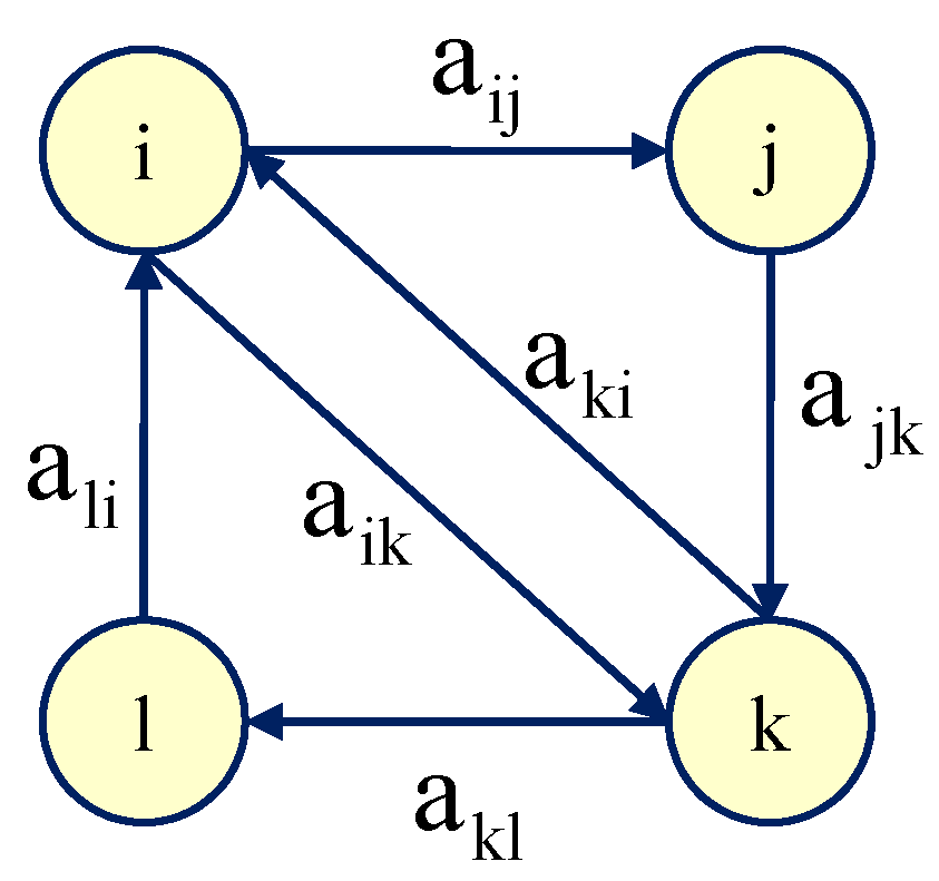
A cycle of length greater than 3 can be easily broken down into product of cycles of length 3. For example (Figure 1 and Figure 2), when $l=4$:

$$a_{ij}{a}_{jk}{a}_{kl}{a}_{li}=a_{ij}{a}_{jk}\left(a_{ki}{a}_{ik}\right)a_{kl}{a}_{li}=\left(a_{ij}{a}_{jk}{a}_{ki}\right)\left(a_{ik\phantom{j}}{a}_{kl}{a}_{li}\right)$$

Therefore, a measure of divergence $d_{ijkl}=f\left(a_{ij}{a}_{jk}{a}_{kl}{a}_{li}\right)$ can be obtained as $d_{ijkl}=f^{\prime }(d_{ijk},d_{ikl})$ and a global measure can be considered as a function of the intensities of the cycles of length 3.

The following result not only allows the expression of the general index $I_l\left(A\right)$ to be obtained in terms of cycles of length 3, but also proves that all indexes $I_l\left(A\right)$ provide the same value regardless of the value of l.

Theorem 2.

Given a pairwise comparison matrix, $A_{\left(nxn\right)}=\left(a_{ij}\right)$ with $a_{ij}{a}_{ji}=1$ and $a_{ij}>0$, it holds that

$$I_l\left(A\right)=GCI\left(A\right)$$

(16)

Proof. 

See Appendix A. □

These cycle-based indices are equivalent, regardless of the cycle length that is considered. Given that the complexity of calculation increases as l increases, it is sufficient to consider the $T\text{-}GCI$ when the objective is to measure the inconsistency from a judgements cycles-based approach.

It can be easily verified that the calculation of the index $I_l\left(A\right)$ has complexity $o\left(n^l\right)$, with n being the order of the matrix A. From a computational point of view, its calculation for $n>3$ will not be of interest. Since all these measures are equal, it is faster to obtain the value of $I_3\left(A\right)=T\text{-}GCI\left(A\right)$.

5. Conclusions

The evaluation of the consistency of decision makers when incorporating their preferences in the AHP, in other words, when eliciting their judgements in pairwise comparison matrices, is one of the most outstanding characteristics of this multi-criteria technique. The initial measures of inconsistency, including the two most widely employed in the scientific literature ($CR$ and $GCI$), were associated with indexes derived for the prioritisation method used (EV and RGM, respectively). Along with this approach, another method, based on triads, is developed. It evaluates the inconsistency using the definition of a consistent pairwise comparison matrix, or equivalently, in terms of the cycles of length 3, comprising the elements of the matrix.

The current paper introduces a new indicator based on triads ($T\text{-}GCI$) that links the two approaches followed in the evaluation of the inconsistency of AHP. As demonstrated in the paper, this indicator coincides with the $GCI$, a measure of inconsistency proposed for the RGM. The relationship between the two indicators can take advantage of the properties and characteristics of both to exploit their potential with regards to calculation.

The work does not analyse the relationship between consistency and representativeness of the priority vector derived from the pairwise comparison matrix. The main objective is to propose a new indicator based on triads, the $T\text{-}GCI$, which links the two approaches considered when defining inconsistency measures and is more efficient than the $GCI$ for matrices with fewer than eight alternatives. This fact is of great significance for simulation studies that require reiterating on numerous occasions the calculation of the inconsistency measure. It is also necessary to emphasise the fact that our work does not deal with obtaining the $T\text{-}GCI$ for incomplete matrices. Studies analysing the estimation of inconsistency for incomplete matrices can be seen in [65,66].

The relationship between the $T\text{-}GCI$ and the $GCI$, and the similarities with different inconsistency measures already proved for the $GCI$, can be used to transfer the results obtained for it to other inconsistency measures, based on triads or the priority vectors; in particular, the setting of thresholds to make those inconsistency indices without thresholds operational. Finally, it has been shown that the generalisation of the $T\text{-}GCI$ to cycles of any length can be expressed in terms of cycles of length 3, which facilitates calculation. Future extensions that are under consideration include how to obtain thresholds for the $T\text{-}GCI$ that would be calculated directly, or obtained in a similar way to the methods for other related indicators.

References

1. Colomer, J.M. Ramon Llull: From ‘Ars electionis’ to social choice theory. Soc. Choice Welf. 2013, 40, 317–328. [Google Scholar] [CrossRef]
2. Fechner, G.; Boring, E.; Howes, D. Elements of Psychophysics; Number v. 1 in Henry Holt Editions in Psychology; Holt, Rinehart and Winston: New York, NY, USA, 1966. [Google Scholar]
3. Thurstone, L.L. A law of comparative judgment. Psychol. Rev. 1927, 34, 273–286. [Google Scholar] [CrossRef]
4. Saaty, T.L. A scaling method for priorities in hierarchical structures. J. Math. Psychol. 1977, 15, 234–281. [Google Scholar] [CrossRef]
5. Saaty, T.L. Multicriteria Decision Making: The Analytic Hierarchy Process; McGraw-Hill: New York, NY, USA, 1980. [Google Scholar]
6. Gerschgorin, S. Über die Abgrenzung der Eigenwerte einer Matrix. Izv. Akad. Nauk. SSSR Ser. Mat. 1931, 7, 749–754. [Google Scholar]
7. Kendall, M.G.; Smith, B.B. On the Method of Paired Comparisons. Biometrika 1940, 31, 324–345. [Google Scholar] [CrossRef]
8. Gerard, H.B.; Shapiro, H.N. Determining the degree of inconsistency in a set of paired comparisons. Psychometrika 1958, 23, 33–46. [Google Scholar] [CrossRef]
9. Vargas, L.G. A note on the eigenvalue consistency index. Appl. Math. Comput. 1980, 7, 195–203. [Google Scholar] [CrossRef]
10. Aguarón, J.; Moreno-Jiménez, J.M. The Geometric Consistency Index: Approximated Thresholds. Eur. J. Oper. Res. 2003, 147, 137–145. [Google Scholar] [CrossRef]
11. Schmidt, F.L.; Hunter, J.E. Theory Testing and Measurement Error. Intelligence 1999, 27, 183–198. [Google Scholar] [CrossRef]
12. Baby, S. AHP modeling for multicriteria decision-making and to optimise strategies for protecting coastal landscape resources. Int. J. Innov. Manag. Technol. 2013, 4, 218–227. [Google Scholar] [CrossRef] [Green Version]
13. Kwiesielewicz, M.; van Uden, E. Inconsistent and contradictory judgements in pairwise comparison method in the AHP. Comput. Oper. Res. 2004, 31, 713–719. [Google Scholar] [CrossRef]
14. Danner, M.; Vennedey, V.; Hiligsmann, M.; Fauser, S.; Gross, C.; Stock, S. How Well Can Analytic Hierarchy Process be Used to Elicit Individual Preferences? Insights from a Survey in Patients Suffering from Age-Related Macular Degeneration. Patient Cent. Outcomes Res. 2016, 9. [Google Scholar] [CrossRef] [PubMed]
15. Bodin, L.; Gass, S.I. On teaching the analytic hierarchy process. Comput. Oper. Res. 2003, 30, 1487–1497. [Google Scholar] [CrossRef]
16. Lipovetsky, S.; Conklin, W.M. Robust estimation of priorities in the AHP. Eur. J. Oper. Res. 2002, 137, 110–122. [Google Scholar] [CrossRef]
17. Dyer, J.S. Remarks on the Analytic Hierarchy Process. Manag. Sci. 1990, 36, 249–258. [Google Scholar] [CrossRef]
18. Koczkodaj, W.; Szwarc, R. On Axiomatization of Inconsistency Indicators for Pairwise Comparisons. Fundam. Inf. 2014, 132, 485–500. [Google Scholar] [CrossRef] [Green Version]
19. Saaty, T.L. How to Make a Decision: The Analytic Hierarchy Process. Interfaces 1994, 24, 19–43. [Google Scholar] [CrossRef]
20. Crawford, G.; Williams, C. A note on the analysis of subjective judgment matrices. J. Math. Psychol. 1985, 29, 387–405. [Google Scholar] [CrossRef]
21. Altuzarra, A.; Moreno-Jiménez, J.M.; Salvador, M. Consensus Building in AHP-Group Decision Making: A Bayesian Approach. Oper. Res. 2010, 58, 1755–1773. [Google Scholar] [CrossRef]
22. Csató, L. Characterization of the Row Geometric Mean Ranking with a Group Consensus Axiom. Group Decis. Negot. 2018, 27, 1011–1027. [Google Scholar] [CrossRef] [Green Version]
23. Csató, L. A characterization of the Logarithmic Least Squares Method. Eur. J. Oper. Res. 2019, 276, 212–216. [Google Scholar] [CrossRef]
24. Golden, B.L.; Wang, Q. An Alternate Measure of Consistency. In The Analytic Hierarchy Process: Applications and Studies; Golden, B.L., Wasil, E.A., Harker, P.T., Eds.; Springer: Berlin/Heidelberg, Germany, 1989; pp. 68–81. [Google Scholar] [CrossRef]
25. Stein, W.; Mizzi, P. The Harmonic Consistency Index for the Analytic Hierarchy Process. Eur. J. Oper. Res. 2007, 177, 488–497. [Google Scholar] [CrossRef]
26. Srdjevic, B. Combining different prioritization methods in the analytic hierarchy process synthesis. Comput. Oper. Res. 2005, 32, 1897–1919. [Google Scholar] [CrossRef]
27. Ramík, J.; Korviny, P. Inconsistency of pair-wise comparison matrix with fuzzy elements based on geometric mean. Fuzzy Sets Syst. 2010, 161, 1604–1613. [Google Scholar] [CrossRef]
28. Kou, G.; Lin, C. A cosine maximization method for the priority vector derivation in AHP. Eur. J. Oper. Res. 2014, 235, 225–232. [Google Scholar] [CrossRef] [Green Version]
29. Koczkodaj, W. A new definition of consistency of pairwise comparisons. Math. Comput. Model. 1993, 18, 79–84. [Google Scholar] [CrossRef]
30. Duszak, Z.; Koczkodaj, W.W. Generalization of a new definition of consistency for pairwise comparisons. Inf. Process. Lett. 1994, 52, 273–276. [Google Scholar] [CrossRef]
31. Peláez, J.; Lamata, M. A new measure of consistency for positive reciprocal matrices. Comput. Math. Appl. 2003, 46, 1839–1845. [Google Scholar] [CrossRef] [Green Version]
32. Shiraishi, S.; Obata, T.; Daigo, M. Properties of a Positive Reciprocal Matrix and their Application to AHP. J. Oper. Res. Soc. Jpn. 1998, 41, 404–414. [Google Scholar] [CrossRef] [Green Version]
33. Dodd, F.; Donegan, H.; McMaster, T. A statistical approach to consistency in AHP. Math. Comput. Model. 1993, 18, 19–22. [Google Scholar] [CrossRef]
34. Jensen, R. Comparison of Eigenvector, Least Squares, Chi Square and Logarithmic Least Squares Methods of Scaling a Reciprocal Matrix; Working Paper 127; Trinity University: San Antonio, TX, USA, 1983. [Google Scholar]
35. Gass, S.; Rapcsák, T. Singular value decomposition in AHP. Eur. J. Oper. Res. 2004, 154, 573–584. [Google Scholar] [CrossRef]
36. Monsuur, H. An intrinsic consistency threshold for reciprocal matrices. Eur. J. Oper. Res. 1997, 96, 387–391. [Google Scholar] [CrossRef]
37. Chu, A.T.W.; Kalaba, R.E.; Spingarn, K. A comparison of two methods for determining the weights of belonging to fuzzy sets. J. Optim. Theory Appl. 1979, 27, 531–538. [Google Scholar] [CrossRef]
38. Wu, Z.; Xu, J. A consistency and consensus based decision support model for group decision making with multiplicative preference relations. Decis. Support Syst. 2012, 52, 757–767. [Google Scholar] [CrossRef]
39. Brunelli, M.; Critch, A.; Fedrizzi, M. A note on the proportionality between some consistency indices in the AHP. Appl. Math. Comput. 2013, 219, 7901–7906. [Google Scholar] [CrossRef] [Green Version]
40. Szybowski, J. The Cycle Inconsistency Index in Pairwise Comparisons Matrices. Procedia Comput. Sci. 2016, 96, 879–886. [Google Scholar] [CrossRef]
41. Brunelli, M. A survey of inconsistency indices for pairwise comparisons. Int. J. Gen. Syst. 2018, 47, 751–771. [Google Scholar] [CrossRef]
42. Cavallo, B. Functional relations and Spearman correlation between consistency indices. J. Oper. Res. Soc. 2020, 71, 301–311. [Google Scholar] [CrossRef]
43. Aguarón, J.; Escobar, M.T.; Moreno-Jiménez, J.M. Reducing Inconsistency measured by the Geometric Consistency Index in the Analytic Hierarchy Process. Eur. J. Oper. Res. 2020. Forthcoming. [Google Scholar]
44. Bozóki, S.; Fülöp, J.; Poesz, A. On reducing inconsistency of pairwise comparison matrices below an acceptance threshold. Cent. Eur. J. Oper. Res. 2015, 23, 849–866. [Google Scholar] [CrossRef] [Green Version]
45. Aguarón, J.; Escobar, M.T.; Moreno-Jiménez, J.M. Consistency Stability Intervals for a judgement in AHP Decision Support Systems. Eur. J. Oper. Res. 2003, 145, 382–393. [Google Scholar] [CrossRef]
46. Moreno-Jiménez, J.M.; Aguarón, J.; Raluy, A.; Turón, A. A Spreadsheet Module for Consistent Consensus Building in AHP-Group Decision Making. Group Decis. Negot. 2005, 14, 89–108. [Google Scholar] [CrossRef]
47. Moreno-Jiménez, J.M.; Aguarón, J.; Escobar, M.T. The Core of Consistency in AHP-Group Decision Making. Group Decis. Negot. 2008, 17, 249–265. [Google Scholar] [CrossRef]
48. Escobar, M.T.; Aguarón, J.; Moreno-Jiménez, J.M. Some extensions of the precise consistency consensus matrix. Decis. Support Syst. 2015, 74, 67–77. [Google Scholar] [CrossRef]
49. Aguarón, J.; Escobar, M.T.; Moreno-Jiménez, J.M. The precise consistency consensus matrix in a local AHP-group decision making context. Ann. Oper. Res. 2016, 245, 245–259. [Google Scholar] [CrossRef]
50. Brunelli, M.; Fedrizzi, M. Axiomatic properties of inconsistency indices for pairwise comparisons. J. Oper. Res. Soc. 2015, 66, 1–15. [Google Scholar] [CrossRef] [Green Version]
51. Brunelli, M.; Fedrizzi, M. Boundary properties of the inconsistency of pairwise comparisons in group decisions. Eur. J. Oper. Res. 2015, 240, 765–773. [Google Scholar] [CrossRef] [Green Version]
52. Brunelli, M. Studying a set of properties of inconsistency indices for pairwise comparisons. Ann. Oper. Res. 2017, 248, 143–161. [Google Scholar] [CrossRef] [Green Version]
53. Bozóki, S.; Rapcsák, T. On Saaty’s and Koczkodaj’s inconsistencies of pairwise comparison matrices. J. Glob. Optim. 2008, 42, 157–175. [Google Scholar] [CrossRef] [Green Version]
54. Csató, L. Axiomatizations of inconsistency indices for triads. Ann. Oper. Res. 2019, 280, 99–110. [Google Scholar] [CrossRef] [Green Version]
55. Cavallo, B.; D’Apuzzo, L. Investigating Properties of the ⊙–Consistency Index. In Advances in Computational Intelligence; Greco, S., Bouchon-Meunier, B., Coletti, G., Fedrizzi, M., Matarazzo, B., Yager, R.R., Eds.; Springer: Berlin/Heidelberg, Germany, 2012; pp. 315–327. [Google Scholar] [CrossRef]
56. Brunelli, M.; Canal, L.; Fedrizzi, M. Inconsistency indices for pairwise comparison matrices: A numerical study. Ann. Oper. Res. 2013, 211, 493–509. [Google Scholar] [CrossRef]
57. Kułakowski, K.; Szybowski, J. The New Triad based Inconsistency Indices for Pairwise Comparisons. Procedia Comput. Sci. 2014, 35, 1132–1137. [Google Scholar] [CrossRef] [Green Version]
58. Koczkodaj, W.; Szybowski, J. Pairwise comparisons simplified. Appl. Math. Comput. 2015, 253, 387–394. [Google Scholar] [CrossRef] [Green Version]
59. Kazibudzki, P. Redefinition of Triad’s Inconsistency and its Impact on the Consistency Measurement of Pairwise Comparison Matrix. J. Appl. Math. Comput. Mech. 2016, 2016, 71–78. [Google Scholar] [CrossRef] [Green Version]
60. Brunelli, M. Recent advances on inconsistency indices for pairwise comparisons—A commentary. Fundam. Inf. 2016, 144, 321–332. [Google Scholar] [CrossRef] [Green Version]
61. Koczkodaj, W.; Urban, R. Axiomatization of inconsistency indicators for pairwise comparisons. Int. J. Approx. Reason. 2018, 94, 18–29. [Google Scholar] [CrossRef] [Green Version]
62. Csató, L. Characterization of an inconsistency ranking for pairwise comparison matrices. Ann. Oper. Res. 2018, 261. [Google Scholar] [CrossRef] [Green Version]
63. Koczkodaj, W.W.; Szybowski, J. The key properties of inconsistency indicators for a triad in pairwise comparison matrices. arXiv 2017, arXiv:1505.05220v2. [Google Scholar]
64. Mazurek, J. Some notes on the properties of inconsistency indices in pairwise comparisons. Oper. Res. Decis. 2018, 1, 27–42. [Google Scholar]
65. Bozóki, S.; Fülöp, J.; Rónyai, L. On optimal completion of incomplete pairwise comparison matrices. Math. Comput. Model. 2010, 52, 318–333. [Google Scholar] [CrossRef] [Green Version]
66. Kułakowski, K.; Talaga, D. Inconsistency indices for incomplete pairwise comparisons matrices. Int. J. Gen. Syst. 2020, 49, 1–27. [Google Scholar] [CrossRef] [Green Version]
Figure 1. Cycle of length 4.
Mathematics 08 00926 g001
Figure 2. Cycles of length 3.
Mathematics 08 00926 g002