Improvement of the Fairness of Non-Preemptive Priorities in the Transmission of Heterogeneous Traffic

Abstract

A new flexible discipline for providing priority to one of two types of customers in a single-server queue is proposed. This discipline assumes the use of additional finite storages for each type of arriving customer. During the stay in a storage, a customer can leave the system or transfer to the main infinite buffer. Preference to priority customers is provided via the proper choice of the rates of a customer transfer from the storages to the buffer. Analysis of this discipline is implemented under quite general assumptions about the arrival and service processes. The advantage of the proposed discipline over the classical non-preemptive discipline is numerically demonstrated.

1. Introduction

Queueing theory provides a powerful tool for the optimization of sharing the restricted resources in many telecommunication, manufacturing, logistic, social, and other systems and networks. In particular, it has wide applications for optimization of routing and energy saving in modern networks where heterogeneous information flows have to be delivered from one node to another one with minimal delay and energy consumption; see, e.g., [1,2,3,4,5,6,7]. The flows are heterogeneous with respect to the required bandwidth (e.g., elephant, dog, and mice flows) and CPU (computationally sparse and computationally dense flows). Very often, the requests receiving service in such systems are inhomogeneous with respect to the indicators of the quality of service (e.g., delay sensitive or insensitive customers, customers tolerant or intolerant to partial loss, streaming or elastic customers, perishable and non-perishable goods, etc.), as well as with respect to their economic or social value. Therefore, certain mechanisms for providing preferences for some types of customers are offered and widely analyzed in the literature. Among these mechanisms, we can mention various polling disciplines with suitably chosen round tables and the maximum attendance times and the generalized processor sharing disciplines. In polling disciplines, which assume a cyclic connection of the common server to the buffers designed for storing different types of customers, priority can be provided to some type of customers via more frequent connection to the buffer for storing the priority customers and via a longer duration of maintaining this connection. The generalized processor sharing discipline is the generalization of the usual processor sharing discipline, which assumes that all customers present in the system receive service simultaneously with the rate inversely proportional to the number of these customers. This generalization assumes that various types of customers can use not equal, but different shares of the capacity of the server.

As a simpler mechanism, which does not permanently require the sharing of time or processor and may be much easier implemented in real-world systems, customer prioritization can be used. Static priorities define the discipline of the choice of the next customer for service based only on the types of customers present in the system. A non-preemptive static priority does not suggest an interruption of non-priority customer service when the priority customer arrives. The preemptive static priority assumes such an interruption. A non-priority customer in this situation may be lost or return to the buffer and later try to receive service again (there exist many variants of the duration of the repeated service). The evident shortcoming of the static priorities is their evident unfairness with respect to the low priority customers, especially in the situation when the real values of the priority and non-priority customers for the system are not essentially different. A low priority customer can have a very long waiting time and succeed to start service essentially later than the priority customer that arrived only recently; see, e.g., [8]. In this respect, the dynamical priorities, which take into account not only the types of customers present in the system, but also the lengths of the corresponding queues, are much more flexible. However, the problems of proving the optimality of some intuitively reasonable strategies (e.g., the threshold or hysteresis) in the class of all available strategies and making the optimal choice of the parameters of the control strategy are, as a rule, quite complicated. Furthermore, what is even more essential is that the practical realization of such a strategy (requiring, in particular, the permanent monitoring of the lengths of queues of all types) can be very difficult or costly.

As some trade-off between the static and dynamic priorities, the disciplines changing (or accumulating) the priority during a customer stay in the queue deserve to be mentioned; see, e.g., [9,10,11,12]. The advantage of such disciplines is that in the case of long waiting in the queue, the non-priority customer may receive a chance to become the priority customer. Another interesting kind of priority queue, in which the contradiction between different types of customers is a bit smoothed out, is queues with space–time priority, in which one type of customer has a priority in the selection of the service from the queue (time priority), while the second one has a priority in the admission to the common buffer space (space priority); see, e.g., [13,14] and the references therein. A simpler discipline, which relaxes the static priority, consists of the randomized choice of the queue from which the next customer is picked for service at the service completion moment. In the case of two priority classes, this discipline includes the strict non-preemptive priority discipline as a particular case. A shortcoming of this discipline consists of the fact that the discipline does not account for the lengths of queues. With a probably small, but positive, probability, the next service can be provided to the very recently arrived low priority customer, while there are many high priority customers waiting in the queue. In [15], essential improvement of such a discipline was considered. The system had one finite and one infinite buffer. The improved discipline assumed the randomized choice of the buffer, from which the next customer would be picked for service, if the number of customers in the finite buffer did not exceed a certain threshold. In the opposite case, the customer from the finite buffer was picked for service.

In this paper, we propose and analyze another reasonable mechanism for customer admission to service that is more flexible than the strict non-preemptive priority. The idea of this mechanism is to introduce some auxiliary storages for the preliminary storing of the different types of arriving customers before their admission to the main buffer. These storages allow smoothing customers’ arrival to the buffer and prevent monopolization of the buffer by the high priority customers. Via the proper choice of the rates of customer transfer from the corresponding storage to the buffer, it is possible to provide enough preference to high priority customers without service discrimination of low priority customers. The analysis of the performance of the system under any fixed set of system parameters is implemented under quite general assumptions about the arrival and service processes. We assume the Marked Markov Arrival Process $\left(MMAP\right)$, which allows accounting for possible correlation in the arrival process, and the Phase-Type (PH) distribution of service time, which allows dealing with the service time having the coefficient of variation different from one.

The outline of the presentation of the results is the following. In Section 2, the mathematical model is completely described. The process of system states is formally defined in Section 3. This process is a multi-dimensional continuous-time Markov chain. This chain belongs to the class of level-independent quasi-birth-and-death processes in the case when the customers staying in the buffer are absolutely patient and to the class of level-dependent quasi-birth-and-death processes (and asymptotically quasi-Toeplitz–Markov chains) when the customers staying in the buffer are impatient. For both cases, ergodicity conditions are proven, and the calculation of the stationary distribution is briefly discussed. Expressions for the key performance indicators of the system are given in Section 4. The results of numerical experiments are presented in Section 5. They highlight the impact of customer transfer rates from the storages to the buffer on the performance measures of the system and illustrate the possibility of the optimal choice of the rates to minimize the weighted loss functions including the probabilities of customer loss in the storages and in the buffer (due to impatience).

2. Mathematical Model

We consider a single-server queueing system with an infinite buffer, the structure of which is presented in Figure 1.

The arrival of two types of customers is defined by the $MMAP$ (see [16]), which is the transparent generalization of the well-known $MAP$ (Markov Arrival Process) (see, e.g., [17,18,19]) to the case of heterogeneous customers. This process is defined by the irreducible continuous-time Markov chain ${\nu }_t,t\ge 0,$ having a finite state space $\{1,2,...,W\}$ and the matrices $D_0,D_1,D_2$ such that the matrix $D_r$ consists of the intensities of transitions of the chain ${\nu }_t$ that are accompanied by the arrival of the type-r customer, $r=1,2.$ The non-diagonal entries of the matrix $D_0$ define the intensity of the corresponding transition of the chain ${\nu }_t$ without the generation of customers, and the modules of the negative diagonal entries define the rates of the exit of the process ${\nu }_t$ from the corresponding states. The matrix $D\left(1\right)=D_0+D_1+D_2$ is the generator of the Markov chain ${\nu }_t.$

The average intensity of customers’ arrival (fundamental rate) $\lambda$ is defined by the formula $\lambda =\theta (D_1+D_2)\mathbf{e},$ where $\theta$ is the row vector of the stationary probabilities of the Markov chain ${\nu }_t.$ This vector is the unique solution to the system $\theta D\left(1\right)=\mathbf{0},\mathbf{\theta }\mathbf{e}=1.$ Here and throughout this paper, $\mathbf{e}$ is a column vector of appropriate size consisting of ones, and $\mathbf{0}$ is a row vector of appropriate size consisting of zeroes. The average intensity of type-r customers’ arrival ${\lambda }_r$ is defined by the formula ${\lambda }_r=\theta D_r\mathbf{e},r=1,2.$ A more detailed description of the $MMAP$ can be found, e.g., in [20].

Upon arrival, type-r customers are placed into the rth storage. The first and the second storages have the finite capacities K and $R,$ correspondingly. Each type-r customer transfers from the storage to the infinite buffer after a random time that is exponentially distributed with the parameter ${\gamma }_r,{\gamma }_r\ge 0,r=1,2.$ We assume that Type-1 customers have a priority over Type-2 customers. This priority is achieved due to the higher rate of transfer from the storage to the buffer. Thus, we assume ${\gamma }_1>{\gamma }_2$.

To avoid starvation of the server and improve the performance of the system, we assume the following. If at a service completion moment, the buffer is empty, but the first storage is not empty, the Type-1 customer is immediately picked up from the storage and starts service. If this storage is empty, but the second storage is not empty, the Type-2 customer is picked up from this storage and starts service. If both storages, as well as the buffer are empty, the server stays idle until the first arrival of a customer of any type. This customer immediately starts service without visiting a storage.

The customers staying in the rth storage are assumed to be impatient. Each type-r customer leaves the corresponding storage (is lost) after an exponentially distributed with the parameter ${\alpha }_r,{\alpha }_r\ge 0,r=1,2,$ amount of time.

After entering the infinite buffer, the customers are assumed to become identical. The service time of an arbitrary customer has a $PH$ distribution with the irreducible representation $(\beta ,S).$ This service time can be interpreted as the time until the underlying Markov process $m_t,t\ge 0,$ with a finite set $\{1,\cdots ,M\}$ of the transient states and the absorbing state $M+1$, reaches the state $M+1$ conditional on the fact that the initial state of this process is selected among the transient states with the probabilities given by the entries of the stochastic row vector $\beta .$ The transition rates of the process $m_t$ within the set $\{1,\cdots ,M\}$ are defined by the sub-generator $S,$ and the transition rates into the absorbing state are given by the entries of the column vector ${\mathbf{S}}_0=-S\mathbf{e}.$ The mean service time is calculated as $b_1=\beta {(-S)}^{-1}\mathbf{e}.$ The mean service rate is $\mu =b_1^{-1}.$ For more details about the $PH$ distribution, see [21]. It is worth noting that the class of $PH$ distributions is dense in the set of distributions of non-negative random variables; see, e.g., [22]. Therefore, this distribution can be used for the approximation of an arbitrary distribution of service time.

The customers staying in the buffer are assumed to be impatient. Each customer, which is not picked up for service, leaves the buffer after an exponentially distributed with the parameter $\phi$ amount of time.

Let us analyze the stochastic process defining the behavior of the described queueing model.

3. Process of System States and Its Stationary Distribution

Let, during the epoch $t,t\ge 0,$

•

$i_t,$$i_t\ge 0,$ be the number of customers in the infinite buffer and on the server,

•

$k_t,$$k_t=\overline{0,K},$ be the number of customers in Storage 1,

•

$r_t,$$r_t=\overline{0,R},$ be the number of customers in Storage 2,

•

${\nu }_t,{\nu }_t=\overline{1,W},$ be the state of the underlying process of the $MMAP,$

•

$m_t,m_t=\overline{1,M},$ be the state of $PH$ service process.

The Markov chain ${\xi }_t=\{i_t,k_t,r_t,{\nu }_t,m_t\},$$t\ge 0,$ is a regular irreducible continuous-time Markov chain. It has the following state space:

$$\left(\{0,0,0,\nu \}\right)\bigcup (\{i,k,r,\nu ,m\},i>0),k=\overline{0,K},r=\overline{0,R},\nu =\overline{1,W},m=\overline{1,M}.$$

Let us introduce the following notations:

•

I is the identity matrix, and O is a zero matrix of an appropriate dimension. If necessary, the dimension of the matrix is indicated by the suffix;

•

$C_l$ is the square matrix of size l defined as follows $C_l=\mathrm{diag}\{0,1,\dots ,l-1\},$ i.e., C is the diagonal matrix with the diagonal entries $\{0,1,\dots ,l-1\},l=K+1,R+1$;

•

$E_l^{-}$ is the square matrix of size l with all zero entries except the entries ${\left(E_l^{-}\right)}_{k,k-1},k=\overline{1,l-1},$ which are equal to one, $l=K+1,R+1$;

•

$E_l^{+}$ is the square matrix of size l with all zero entries except the entries ${\left(E_l^{+}\right)}_{k,k+1},k=\overline{0,l-2},$ and ${\left(E_l^{+}\right)}_{l-1,l-1}$, which are equal to one, $l=K+1,R+1$;

•

${\widehat{I}}_l$ is the square matrix of size l with all zero entries except the entry ${\left({\widehat{I}}_l\right)}_{0,0}$, which is equal to one, $l=K+1,R+1$;

•

${\mathit{a}}_l$ is the row vector of size l with all zero entries except the entry ${\left({\mathit{a}}_l\right)}_0$, which is equal to one, $l=K+1,R+1$;

•

⊗ and ⊕ are the symbols of the Kronecker product and the sum of matrices; see, e.g., [23].

Let us enumerate the states of the Markov chain ${\xi }_t$ in the lexicographic order and refer to the set of states of the chain having value i of the first component of the Markov chain as level $i,i\ge 0.$

Let Q be the generator of the Markov chain ${\xi }_t,t\ge 0.$

Lemma 1.

The generator Q has the following block-tridiagonal structure:

$$Q=\left(\begin{array}{ccccccc}{Q}_{0,0}& Q_{0,1}& O& O& O& O& \dots \\ Q_{1,0}& Q_{1,1}& Q^{+}& O& O& O& \dots \\ O& Q_{2,1}& Q_{2,2}& Q^{+}& O& O& \dots \\ O& O& Q_{3,2}& Q_{3,3}& Q^{+}& O& \dots \\ ⋮& ⋮& ⋮& ⋮& ⋮& ⋮& \ddots \end{array}\right).$$

The non-zero blocks $Q_{i,j},i,j\ge 0,$ containing the intensities of the transitions from level i to level j have the following form:

$$Q_{0,0}=D_0,$$

$$Q_{0,1}={\mathit{a}}_{K+1}\otimes {\mathit{a}}_{R+1}\otimes (D_1+D_2)\otimes \mathit{\beta },$$

$$Q_{1,1}=I_{(K+1)(R+1)}\otimes (D_0\oplus S)+E_{K+1}^{+}\otimes I_{R+1}\otimes D_1\otimes I_M+I_{K+1}\otimes E_{R+1}^{+}\otimes D_2\otimes I_M-$$

$$({\alpha }_1+{\gamma }_1)C_{K+1}\otimes I_{(R+1)WM}-({\alpha }_2+{\gamma }_2)I_{K+1}\otimes C_{R+1}\otimes I_{WM}+$$

$${\alpha }_1{C}_{K+1}{E}_{K+1}^{-}\otimes I_{(R+1)WM}+{\alpha }_2{I}_{K+1}\otimes C_{R+1}{E}_{R+1}^{-}\otimes I_{WM}+(E_{K+1}^{-}\otimes I_{R+1}+{\widehat{I}}_{K+1}\otimes E_{R+1}^{-})\otimes I_W\otimes {\mathit{S}}_0\mathit{\beta },$$

$$Q_{i,i}=I_{(K+1)(R+1)}\otimes (D_0\oplus S)+E_{K+1}^{+}\otimes I_{R+1}\otimes D_1\otimes I_M+I_{K+1}\otimes E_{R+1}^{+}\otimes D_2\otimes I_M-(i-1)\phi I_{(K+1)(R+1)WM}-$$

$$({\alpha }_1+{\gamma }_1)C_{K+1}\otimes I_{(R+1)WM}-({\alpha }_2+{\gamma }_2)I_{K+1}\otimes C_{R+1}\otimes I_{WM}+$$

$${\alpha }_1{C}_{K+1}{E}_{K+1}^{-}\otimes I_{(R+1)WM}+{\alpha }_2{I}_{K+1}\otimes C_{R+1}{E}_{R+1}^{-}\otimes I_{WM},i\ge 2,$$

$$Q_{i,i+1}=Q^{+}={\gamma }_1{C}_{K+1}{E}_{K+1}^{-}\otimes I_{(R+1)WM}+{\gamma }_2{I}_{K+1}\otimes C_{R+1}{E}_{R+1}^{-}\otimes I_{WM},i\ge 1,$$

$$Q_{1,0}={\left({\mathit{a}}_{K+1}\right)}^T\otimes {\left({\mathit{a}}_{R+1}\right)}^T\otimes I_W\otimes {\mathit{S}}_0,$$

$$Q_{i,i-1}=I_{(K+1)(R+1)W}\otimes {\mathit{S}}_0\mathit{\beta }+(i-1)\phi I_{(K+1)(R+1)WM},i>1.$$

The proof of the lemma is performed by means of the analysis of the intensities of all possible transitions of the Markov chain ${\xi }_t$ during the time interval having infinitesimal length. Its brief outline is as follows. The block-tridiagonal form of the generator Q is easily explained by the fact that customers of both types arrive at the system and depart from it (due to service completion or impatience) one by one.

When the server is idle (by default, the buffer and both storages are empty), the dynamics of the Markov chain ${\xi }_t$ is defined only by the process ${\nu }_t.$ The intensities of its transitions to another states are defined by the non-diagonal entries of the matrix $D_0$, and the intensities of the exit from the corresponding states are defined, up to the sign, by the diagonal entries of this matrix. Therefore, $Q_{0,0}=D_0.$

The form of the block $Q_{0,1}$ is explained as follows. This block contains the rates of transition of the Markov chain ${\xi }_t$ when the number of customers in the system increases from zero to one. This happens when the customer of any type arrives. The intensities of the transition of the underlying process ${\nu }_t$ at the arrival moment are defined by the entries of the matrix $D_1+D_2.$ The arrived customer starts service. The initial state of the underlying process of service is selected according to the probabilities given by the entries of the vector $\mathit{\beta }.$ Because the server is not idle after the customer arrival, generally speaking, the storages may be non-empty, and we have to start accounting for the number of customers in both storages. Indeed, the number of customers in both servers remains equal to zero, but we have to declare the start of accounting formally. The matrix ${\mathit{a}}_{K+1}\otimes {\mathit{a}}_{R+1}$ defines that after the customer arrival, both storages remain empty. The symbol ⊗ of the Kronecker product of matrices is very useful to define the transition probabilities or intensities of several independent Markov processes. Summarizing our analysis, we conclude that the block $Q_{0,1}$ has the form $Q_{0,1}={\mathit{a}}_{K+1}\otimes {\mathit{a}}_{R+1}\otimes (D_1+D_2)\otimes \mathit{\beta }.$

Now, let us explain the form of the block $Q_{i,i+1}=Q^{+},i\ge 1.$ The increase of the number of customers in the buffer (including the one in service) from the value i to the value $i+1$ can happen when some customer from Storage 1 or 2 transits to the infinite buffer. The matrix ${\gamma }_1{C}_{K+1}$ defines the intensities of the transition of the customers from Storage 1 to the buffer. Here, the scalar ${\gamma }_1$ defines the rate of transition of an arbitrary Type-1 customer from the storage to the buffer. The diagonal matrix $C_{K+1}$ accounts for the fact that the total transition rate from Storage 1 to the buffer is proportional to the current number of customers in Storage 1. At the moment of transition of an arbitrary Type-1 customer from the storage to the buffer, the number of customers in Storage 1 decreases by one. This transition of the number of customers in Storage 1 is described by the matrix $E_{K+1}^{-}.$ Because transition from Storage 1 to the buffer happened, transitions of any other components during the infinitesimal interval are not possible, i.e., that components remain in their previous states. Thus, transition rates of the Markov chain ${\xi }_t$ from the state having value i of the first component of the chain to the state having value $i+1$ of that component when the customer from Storage 1 transits to the buffer are given by the matrix ${\gamma }_1{C}_{K+1}{E}_{K+1}^{-}\otimes I_{(R+1)WM}.$ It is easy to understand that the corresponding transition rates when the customer from Storage 2 transits to the buffer are given by the matrix ${\gamma }_2{I}_{K+1}\otimes C_{R+1}{E}_{R+1}^{-}\otimes I_{WM}$. As the result, we obtain the formula presented above for the block $Q_{i,i+1}.$

Now, let us explain the form of the block $Q_{i,i-1},i>1.$ The transition of the Markov chain ${\xi }_t$ from the state having value i of the first component of the chain to the state having value $i-1$ of that component is possible when the current service is completed and new service starts (the corresponding transition rates of the chain are given by the matrix $I_{(K+1)(R+1)W}\otimes {\mathit{S}}_0\beta$) or one of $i-1$ customers waiting in the buffer departs from the system due to impatience (the corresponding transition rates of the chain are given by the matrix $(i-1)\phi I_{(K+1)(R+1)WM}$). As a result of this analysis, we obtain the formula presented above for the block $Q_{i,i-1},i>1.$ When $i=1$, because the customer was the only one in the system, we have to take into account that:

(i)

After service completion, new service does not start. Thus, instead of the matrix ${\mathit{S}}_0\beta$, we have the column-vector ${\mathit{S}}_0.$

(ii)

The server becomes idle, the buffer empty, and by default, the storages empty. Therefore, we have to postpone the monitoring of the number of customers in the storages. This can be done by means of using the multiplier ${\left({\mathit{a}}_{K+1}\right)}^T\otimes {\left({\mathit{a}}_{R+1}\right)}^T$ in the transition probability block $Q_{1,0}.$

Now, we have to explain the form of the block $Q_{i,i},i>1.$ This is the diagonal block of the generator. Therefore, all its diagonal entries are negative, and the modules of these entries define the intensities of the exit of the Markov chain ${\xi }_t$ from the corresponding states. The exit of the Markov chain ${\xi }_t$ from the state having value i of the first component is possible in the following ways:

(i)

Underlying processes ${\nu }_t$ of arrivals or $m_t$ of service leave their current states. Corresponding transition intensities of the two-dimensional process $({\nu }_t,m_t)$ are defined, up to the sign, by the diagonal entries of the matrix $D_0\oplus S=D_0\otimes I_M+I_W\otimes S.$

(ii)

Any customer leaves Storage 1 and transits to the buffer or departs from the system due to impatience. Corresponding rates of the exit of the process ${\xi }_t$ from its states are given by the matrix $({\alpha }_1+{\gamma }_1)C_{K+1}\otimes I_{(R+1)WM}.$

(iii)

Any customer leaves Storage 2 and transits to the buffer or departs from the system due to impatience. Corresponding rates of the exit of the process ${\xi }_t$ from its states are given by the matrix $({\alpha }_2+{\gamma }_2)I_{K+1}\otimes C_{R+1}\otimes I_{WM}.$

The non-diagonal entries of the matrix $Q_{i,i}$ define the intensities of the transitions of the Markov chain ${\xi }_t$ without the change of the value i of the first component. These transitions are defined by:

(i)

non-diagonal entries of the matrix $I_{(K+1)(R+1)}\otimes (D_0\oplus S)$ when one of the processes ${\nu }_t$ or $m_t$ makes a transition without customer arrival or service completion.

(ii)

entries of the matrix $E_{K+1}^{+}\otimes I_{R+1}\otimes D_1\otimes I_M$ when a new Type-1 customer arrives and occupies the place in Storage 1.

(iii)

entries of the matrix $I_{K+1}\otimes E_{R+1}^{+}\otimes D_2\otimes I_M$ when a new Type-2 customer arrives and occupies the place in Storage 2.

(iv)

entries of the matrix ${\alpha }_1{C}_{K+1}{E}_{K+1}^{-}\otimes I_{(R+1)WM}$ when a Type-1 customer departs Storage 1 due to impatience.

(v)

entries of the matrix ${\alpha }_2{I}_{K+1}\otimes C_{R+1}{E}_{R+1}^{-}\otimes I_{WM}$ when a Type-2 customer departs Storage 2 due to impatience.

As a result of these derivations, we prove the form of the blocks $Q_{i,i},i>1,$ presented above.

The derivation of the formula for the block $Q_{1,1}$ is similar. One can pay attention to the additional summand $(E_{K+1}^{-}\otimes I_{R+1}+{\widehat{I}}_{K+1}\otimes E_{R+1}^{-})\otimes I_W\otimes {\mathit{S}}_0\beta$ that was absent in the blocks $Q_{i,i},i>1.$ The presence of this block is explained as follows. For $i\ge 1,$ the variant of service completion was not considered at all because mandatory service completion causes the decrease of the value of the first component of the chain from i to $i-1.$ However, when $i=1,$ this variant is possible because it was stated in the model formulation that when the server becomes idle while the buffer is empty, immediately, a new customer is picked up from Storage 1, if it is not empty. If it is empty while Storage 2 is not empty, a new customer is picked up from Storage 2. The matrix $(E_{K+1}^{-}\otimes I_{R+1}+{\widehat{I}}_{K+1}\otimes E_{R+1}^{-})$ describes the transition probabilities of the number of customers in Storages 1 and 2 in such a situation. The Kronecker multiplier $I_W\otimes {\mathit{S}}_0\beta$ defines the intensities of the transition of the two-dimensional process $({\nu }_t,m_t)$ at the moment of service completion and starting a new service. The lemma is proven.

Let us obtain the ergodicity condition of the chain ${\xi }_t.$ Let us introduce the following denotations:

$$F_1=\left(C_{K+1}(E_{K+1}^{-}-I_{K+1})\right)\otimes I_{R+1},$$

$$F_2=I_{K+1}\otimes \left(C_{R+1}(E_{R+1}^{-}-I_{R+1})\right),$$

$$\mathcal{F}=I_{(K+1)(R+1)}\otimes D_0+E_{K+1}^{+}\otimes I_{R+1}\otimes D_1+I_{K+1}\otimes E_{R+1}^{+}\otimes D_2+({\alpha }_1+{\gamma }_1)F_1\otimes I_W+({\alpha }_2+{\gamma }_2)F_2\otimes I_W.$$

Theorem 1.

If the customers in the buffer are impatient ($\phi >0$), the Markov chain ${\xi }_t$ is ergodic for any set of the system parameters.

If the customers in the buffer are patient ($\phi =0$), the Markov chain ${\xi }_t$ is ergodic, if and only if the following inequality is fulfilled:

$$\mathbf{u}\left(({\gamma }_1{C}_{K+1}{E}_{K+1}^{-}\otimes I_{R+1}+{\gamma }_2{I}_{K+1}\otimes C_{R+1}{E}_{R+1}^{-})\otimes I_W\right)\mathbf{e}<\mu$$

(1)

where the vector $\mathbf{u}$ is the unique solution to the system:

$$\mathbf{u}\mathcal{F}=\mathbf{0},\mathbf{u}\mathbf{e}=1.$$

(2)

Proof. 

(1) Let us first consider the case $\phi \ne 0.$ It is easily verified that in this case, the following limits exist:

$$Y_0=\underset{i\to \infty }{lim}{R}_i^{-1}{Q}_{i,i-1}=I,Y_1=\underset{i\to \infty }{lim}{R}_i^{-1}{Q}_{i,i}+I=O,Y_2=\underset{i\to \infty }{lim}{R}_i^{-1}{Q}_{i,i+1}=O$$

where the matrix $R_i$ is a diagonal matrix with the diagonal entries defined as the moduli of the corresponding diagonal entries of the matrix $Q_{i,i},i\ge 0.$ Therefore, according to the definition of continuous-time asymptotically quasi-Toeplitz–Markov chains ($AQTMC$) given in [24], the Markov chain ${\xi }_t,t\ge 0,$ belongs to the class $AQTMC$. As follows from [24], a sufficient condition for the ergodicity of the Markov chain ${\xi }_t$ is the fulfillment of the inequality:

$$\mathbf{y}{Y}_0\mathbf{e}>\mathbf{y}{Y}_2\mathbf{e}$$

(3)

where the vector $\mathbf{y}$ is the unique solution to the system:

$$\mathbf{y}(Y_0+Y_1+Y_2)=\mathbf{y},\mathbf{y}\mathbf{e}=1.$$

Because $Y_0=I,Y_1=O,Y_2=O,$ it is easily observed that Condition (3) holds true for all possible values of the system parameters.

(2) Let us consider the case $\phi =0.$ In this case, the blocks of the generator for $i\ge 2$ have the following form:

$$Q_{i,i}=Q_{2,2},Q_{i,i+1}=Q^{+},Q_{i,i-1}=Q_0,i\ge 2,$$

and:

$$Q_{2,2}+Q^{+}=\mathcal{F}\otimes I_M+I_{(K+1)(R+1)W}\otimes S,$$

$$Q_0=I_{(K+1)(R+1)W}\otimes {\mathit{S}}_0\mathit{\beta }.$$

Since the blocks of the generator do not depend on the variable i when $i\ge 2,$ the Markov chain ${\xi }_t,t\ge 0,$ belongs to the class of continuous-time quasi-Toeplitz–Markov chains ($QTMC$) or $M/G/1$-type Markov chains; see [21]. As follows from [21], the necessary and sufficient condition for the ergodicity of the $QTMC$ is the fulfillment of:

$$\mathbf{z}{Q}^{+}\mathbf{e}<\mathbf{z}{Q}_0\mathbf{e}$$

(4)

where the vector $\mathbf{z}$ is the unique solution to the system:

$$\mathbf{z}(Q_0+Q_{2,2}+Q^{+})=\mathbf{0},\mathbf{z}\mathbf{e}=1.$$

(5)

Let the row vector $\eta$ be the unique solution to the system:

$$\mathit{\eta }(S+{\mathbf{S}}_0\mathit{\beta })=\mathbf{0},\mathit{\eta }\mathbf{e}=1.$$

It is easy to check that the solution of this system is given by:

$$\eta =\mu \beta {(-S)}^{-1}.$$

By direct substitution into (5) and using the so-called mixed product rule for the Kronecker product of matrices, it is possible to check that the vector $\mathbf{z}$ can be represented in the form:

$$\mathbf{z}=\mathbf{u}\otimes \eta$$

(6)

where the vector $\mathbf{u}$ is the solution of System (2). Taking into account (6), we easily obtain that the right-hand side of Inequality (4) is equal to $\mu .$ The left-hand side of Inequality (4) is equal to the left-hand side of inequality (1). Theorem 1 is proven. □

Remark 1.

The vector $\mathbf{u}$ defines the joint distribution of the number of customers in the storages and the underlying process of the $MMAP$ during the time intervals when the system is overloaded, i.e., the number of customers in the buffer is huge. Correspondingly, the expression in the left-hand side of Inequality (1) defines the average rate of customers’ arrival to the buffer when the system is overloaded. Therefore, the meaning of (1) is that the mean arrival rate is less than the mean service rate when the system is overloaded.

Remark 2.

It can be verified that the vector $\mathbf{u}$ defines the joint distribution of the number of customers and the underlying process of $MMAP$ in the queueing system with the $MMAP$ arrival process, two parallel stations containing K and R servers, correspondingly, no buffers, and the exponential service time distribution having the intensity ${\alpha }_r+{\gamma }_r,r=1,2.$ The marginal distribution of the number of busy servers and the state of the underlying process of arrivals at the rth station coincide with such a distribution for the Erlang loss model of the $MAP/M/N_r/N_r$ type where $N_1=K$ and $N_2=R,$ the service time at the rth station having the exponential distribution with the rate ${\alpha }_r+{\gamma }_r$ and $MAP$ defined by the matrices ${\tilde{D}}_0^{\left(r\right)}=D_0+D_{\overline{r}}$ and ${\tilde{D}}_1^{\left(r\right)}=D_r,r,\overline{r}=1,2,r\ne \overline{r}.$

In this case, if the arrival process is the mixture of two independent stationary Poisson processes with the rates ${\lambda }_1$ and ${\lambda }_2,$ correspondingly, these marginal distributions are defined by the probabilities:

$$\frac{\frac{{\delta }_r^k}{k!}}{\sum _{l=0}^{N_r}\frac{{\delta }_r^l}{l!}},k=\overline{0,N_r},$$

where ${\delta }_r=\frac{{\lambda }_r}{{\alpha }_r+{\gamma }_r}.$ The joint distribution of two stations’ states is defined here by the product of the marginal distributions.

Remark 3.

It is worth making the following observation. In the majority of queueing models with the $MMAP$ and its partial case $MAP$ (Markov Arrival Process), the ergodicity condition includes only the average arrival rates and does not depend, e.g., on the correlation of successive inter-arrival times and their variance. This is easily explained by the fact that the stability condition imposes restrictions on the system parameters in the situation when the system is overloaded. In such a situation, the queue length (or the number of customers in the orbit in retrial queues) is very large, and the concrete pattern of the arrival process does not matter. All arriving customers join the long queue, and the distribution and correlation of inter-arrival times (under the fixed average inter-arrival time) do not have an impact. In the model considered in this paper, the stability condition depends not only on the average arrival rate, but on the pattern of the arrival process as well. This is explained by the fact that the overloading of the buffer does not imply the overloading of the storages, and the distribution of the number of customers in the storages may essentially depend on the pattern of $MMAP.$ However, this distribution essentially affects the input flow to the buffer (including the average input rate) and, therefore, the form of the stability condition.

Let the ergodicity condition be fulfilled. Then, the following limits (stationary probabilities) exist:

$$\pi (0,0,0,\nu )=\underset{t\to \infty }{lim}P\{i_t=0,k_t=0,r_t=0,{\nu }_t=\nu \},$$

$$\pi (i,k,r,\nu ,m)=\underset{t\to \infty }{lim}P\{i_t=i,k_t=k,r_t=r,{\nu }_t=\nu ,m_t=m\},$$

$$i>0,k=\overline{0,K},r=\overline{0,R},\nu =\overline{1,W},m=\overline{1,M}.$$

Let us form the row vectors $\pi (i,k,r),\pi (i,k),{\pi }_i$ of these probabilities as follows:

$$\pi (i,k,r,\nu )=(\pi (i,k,r,\nu ,1),\pi (i,k,r,\nu ,2),\dots ,\pi (i,k,r,\nu ,M)),i\ge 1,\nu =\overline{1,W},$$

$$\pi (i,k,r)=(\pi (i,k,r,1),\pi (i,k,r,2),\dots ,\pi (i,k,r,W)),i\ge 1,k=\overline{0,K},r=\overline{0,R},$$

$$\pi (i,k)=(\pi (i,k,0),\pi (i,k,1),\dots ,\pi (i,k,R)),i\ge 1,k=\overline{0,K},$$

$$\pi (0,0,0)=\left(\pi \right(0,0,0,1),\pi (0,0,0,2),\dots ,\pi (0,0,0,W\left)\right),$$

$$\pi (0,0)=\pi (0,0,0),$$

$${\pi }_0=\pi (0,0),$$

$${\pi }_i=(\pi (i,0),\pi (i,1),\dots ,\pi (i,K)),i\ge 1.$$

It is well known that the probability vectors ${\pi }_i,i\ge 0,$ satisfy the following system of linear algebraic equations:

$$({\pi }_0,{\pi }_1,\cdots )Q=\mathbf{0},({\pi }_0,{\pi }_1,\cdots )\mathbf{e}=1$$

called equilibrium or Chapman–Kolmogorov equations. This system is infinite. In the case of absolutely patient customers in the buffer, the solution of this system can be found in the well-known matrix geometric form. If the customers in the buffer are impatient, the generator Q does not possess the Toeplitz-like property. Therefore, the system cannot be directly solved on a computer and does not have a solution in the matrix geometric form; see [21]. Such a type of equation without the Toeplitz-like property of the generator quite often arises in the analysis of queues with impatient customers and retrial queueing systems. In the existing literature, they are usually solved by means of various truncation methods. However, this system can be effectively solved by means of the numerically stable algorithm presented in [25].

4. Performance Measures of the System

Having computed the vectors of the stationary probabilities ${\pi }_i,i\ge 0,$ it is possible to compute a variety of the performance measures of the system.

The average number of customers in the system is computed by:

$$L=\sum _{i=1}^{\infty }\sum _{k=0}^K\sum _{r=0}^R(i+k+r)\pi (i,k,r)\mathbf{e}.$$

The average number of customers in the buffer is computed by:

$$N^{buf}=\sum _{i=2}^{\infty }(i-1){\pi }_i\mathbf{e}.$$

The average number of customers in Storage 1 is computed by:

$$N_1^{stor}=\sum _{i=1}^{\infty }\sum _{k=1}^{K}k\pi (i,k)\mathbf{e}.$$

The average number of customers in Storage 2 is computed by:

$$N_2^{stor}=\sum _{i=1}^{\infty }\sum _{k=0}^K\sum _{r=1}^{R}r\pi (i,k,r)\mathbf{e}.$$

The loss probability of an arbitrary priority customer upon arrival due to Storage 1 overflow is computed by:

$$P_1^{ent-loss}=\frac{1}{{\lambda }_1}\sum _{r=0}^R\sum _{i=1}^{\infty }\pi (i,K,r)(D_1\otimes I_M)\mathbf{e}.$$

The loss probability of an arbitrary non-priority customer upon arrival due to Storage 2 overflow is computed by:

$$P_2^{ent-loss}=\frac{1}{{\lambda }_2}\sum _{k=0}^K\sum _{i=1}^{\infty }\pi (i,k,R)(D_2\otimes I_M)\mathbf{e}.$$

The loss probability of an arbitrary priority customer due to impatience in Storage 1 is computed by:

$$P_1^{imp-loss}=\frac{1}{{\lambda }_1}\sum _{i=1}^{\infty }\sum _{k=1}^{K}k{\alpha }_1\pi (i,k)\mathbf{e}=\frac{{\alpha }_1}{{\lambda }_1}{N}_1^{stor}.$$

The loss probability of an arbitrary non-priority customer due to impatience in Storage 2 is computed by:

$$P_2^{imp-loss}=\frac{1}{{\lambda }_2}\sum _{i=1}^{\infty }\sum _{k=0}^K\sum _{r=1}^{R}r{\alpha }_2\pi (i,k,r)\mathbf{e}=\frac{{\alpha }_2}{{\lambda }_2}{N}_2^{stor}.$$

The intensity of the output flow of successfully served customers is computed by:

$${\lambda }_{out}=\sum _{i=1}^{\infty }{\pi }_i({\mathbf{e}}_{(K+1)(R+1)W}\otimes {\mathit{S}}_0).$$

The probability of an arbitrary customer loss is computed by:

$$P_{loss}=1-\frac{{\lambda }_{out}}{\lambda }.$$

(7)

The probability of an arbitrary priority customer loss from Storage 1 is computed by:

$$P_1^{loss}=P_1^{ent-loss}+P_1^{imp-loss}.$$

The probability of an arbitrary non-priority customer loss from Storage 2 is computed by:

$$P_2^{loss}=P_2^{ent-loss}+P_2^{imp-loss}.$$

The intensity of the input flow of customers into the system (to the buffer or directly to the server) is computed by:

$${\lambda }_{in}=(1-P_1^{loss}){\lambda }_1+(1-P_2^{loss}){\lambda }_2.$$

The loss probability of an arbitrary customer due to impatience in the system is computed by:

$$P^{imp-loss}=\frac{1}{{\lambda }_{in}}\sum _{i=2}^{\infty }(i-1)\phi {\pi }_i\mathbf{e}.$$

Remark 4.

The alternative to Formula (7) for the computation of the probability $P_{loss}$ of an arbitrary customer loss is:

$$P_{loss}=\frac{{\lambda }_1{P}_1^{loss}+{\lambda }_2{P}_2^{loss}+{\lambda }_{in}{P}^{imp-loss}}{\lambda }.$$

The existence of two different formulas for the probability $P_{loss}$ can be helpful for the verification of the results of calculation of the stationary distribution of the Markov chain ${\xi }_t.$

5. Numerical Example

In this numerical example, we investigate the impact of the parameters ${\gamma }_r,r=1,2,$ which define the rates of type-r customers’ transition from the corresponding storage to the infinite buffer, on the main performance measures of the system. The main goal of the numerical example is to show how to optimize the access of priority and non-priority customers via appropriately choosing the parameters ${\gamma }_r,r=1,2.$

Let us assume that the arrival flow of customers is modeled by the $MMAP$ arrival process defined by the following matrices:

$$D_0=\left(\begin{array}{cc}-6.759& 0\\ 0& -0.21941\end{array}\right),D_1=\left(\begin{array}{cc}2.238& 0.015\\ 0.04072& 0.03242\end{array}\right),D_2=\left(\begin{array}{cc}4.476& 0.03\\ 0.08144& 0.06483\end{array}\right).$$

The total rate of customers’ (priority and non-priority) arrival to the system is $\lambda =4.99852.$ The coefficient of correlation of successive inter-arrival times in this arrival process is $0.2,$ and the squared coefficient of variation is $12.3467$. The average intensity of priority customers’ arrival is ${\lambda }_1=1.66617,$ and the average intensity of non-priority customers arrival is ${\lambda }_2=3.33235$.

We assume that the capacity of Storage 1 is $K=5$ and the capacity of Storage 2 is $R=7.$ The intensities of impatience in Storages 1 and 2 are equal to ${\alpha }_1=0.05$ and ${\alpha }_2=0.04,$ and the intensity $\phi$ of impatience in the buffer is equal to $0.06.$ The $PH$ service process is defined by the vector $\beta =(0.1,0.9)$ and the matrix $S=\left(\begin{array}{cc}-5& 0.2\\ 0.5& -8\end{array}\right).$ The mean service time is $b_1=0.144612.$

Let us vary the intensity ${\gamma }_1$ over the interval [0,5] with a step of 0.1. The intensity ${\gamma }_2$ is varied over the interval $[0,{\gamma }_1]$ also with the step of 0.1. For the computations, we use a computer with an Intel Core i7-8700 CPU and 16 GB RAM and Mathematica 11. In this numerical example, the number of different pairs ${\gamma }_1,{\gamma }_2$ is equal to 1326. The total computation time (for all different pairs ${\gamma }_1,{\gamma }_2$) is about 20 min, and the computation time for the fixed values of ${\gamma }_1,{\gamma }_2$ is less than 1 s.

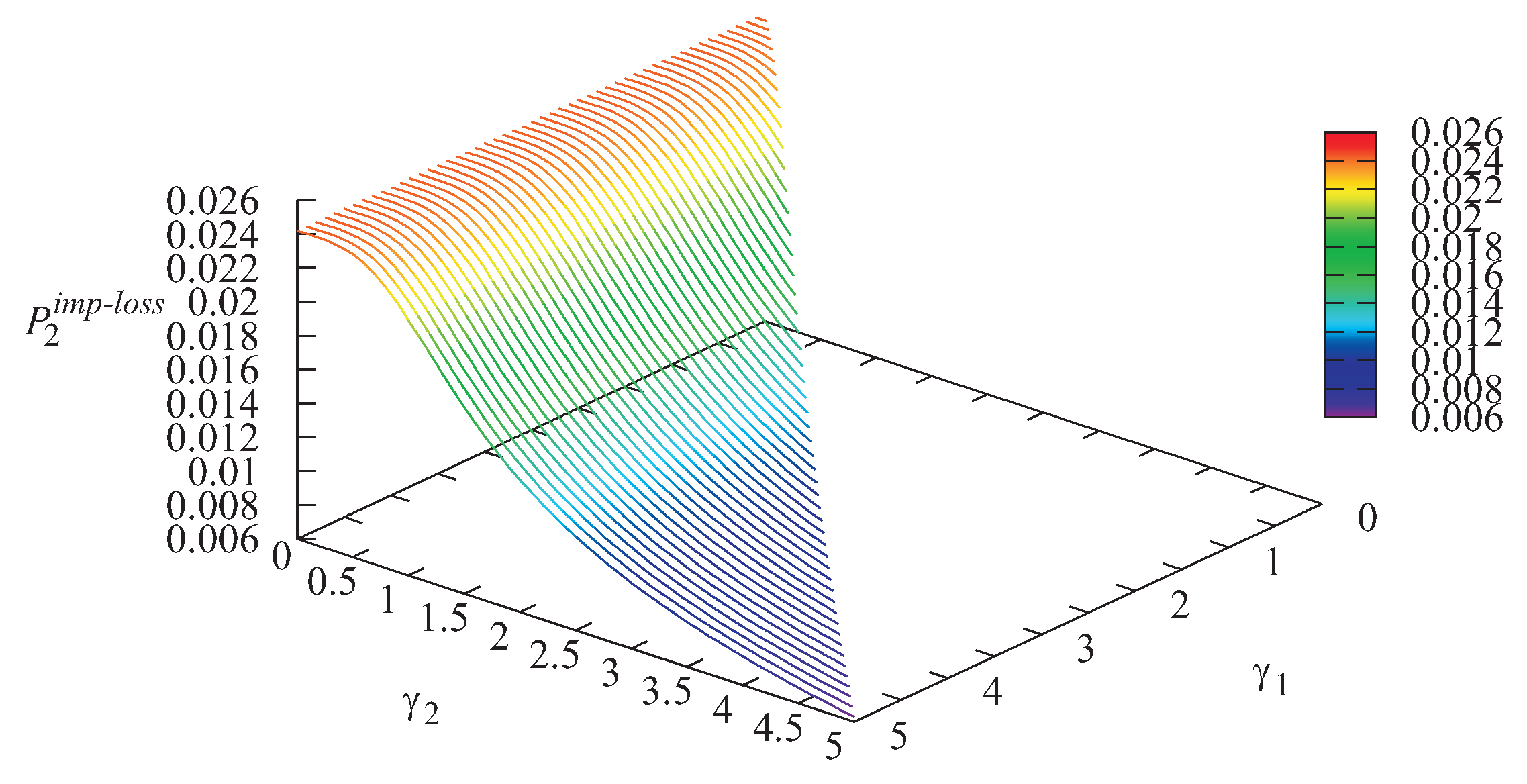
The dependencies of the loss probability $P_1^{ent-loss}$ of an arbitrary priority customer upon arrival due to Storage 1 overflow and the loss probability $P_2^{ent-loss}$ of an arbitrary non-priority customer upon arrival due to Storage 2 overflow on different values of ${\gamma }_1$ and ${\gamma }_2$ are illustrated in Figure 2 and Figure 3. The dependencies of the loss probability $P_1^{imp-loss}$ of an arbitrary priority customer due to impatience in Storage 1 and the loss probability $P_2^{imp-loss}$ of an arbitrary non-priority customer due to impatience in Storage 2 on different values of ${\gamma }_1$ and ${\gamma }_2$ are illustrated in Figure 4 and Figure 5.

As is seen from Figure 2, the loss probability $P_1^{ent-loss}$ of a priority customer due to Storage 1 overflow grows when the intensity ${\gamma }_2$ increases. This is easily explained by the fact that with the increase of ${\gamma }_2$, the loss probabilities of Type-2 customers due to buffer overflow and due to impatience essentially decrease; see Figure 3 and Figure 5. Thus, more Type-2 customers arrive at the infinite buffer, and the server becomes idle less often, while Type-1 customers are rarely chosen from Storage 1 for service without visiting the infinite buffer. Therefore, the number of Type-1 customers in the buffer grows, which causes the increase of the loss probability $P_1^{ent-loss}$. For the same reasons, the growth of the probability $P_1^{imp-loss}$ with the increase of the intensity ${\gamma }_2$ (see Figure 4) can be explained.

The dependencies of the probability $P_1^{loss}$ of an arbitrary priority customer loss from Storage 1 and the probability $P_2^{loss}$ of an arbitrary non-priority customer loss from Storage 2 on different values of ${\gamma }_1$ and ${\gamma }_2$ are illustrated in Figure 6 and Figure 7.

It is seen from Figure 6 that the minimal value of the loss probability of an arbitrary priority customer from Storage 1 is achieved when ${\gamma }_2=0.$ Note, that if ${\gamma }_2=0,$ then Type-2 customers cannot transit to the infinite buffer. Thus, a Type-2 customer can be chosen for service only in the case of the absence of Type-1 customers in the storage and system. Thus, if ${\gamma }_2=0,$ the system under study behaves as some kind of system with non-preemptive priority of Type-1 customers over Type-2 customers. If we fix ${\gamma }_1={\gamma }_2=0,$ we obtain the system with two finite buffers and non-preemptive priority. If we choose huge ${\gamma }_1$ and ${\gamma }_2=0,$ we obtain the system with the finite buffer for non-priority customers, the infinite buffer for priority customers, and non-preemptive priority. However, when ${\gamma }_2$ is equal to zero, the loss probability of Type-2 customers is very high; see Figure 7.

The dependencies of the loss probability $P^{imp-loss}$ of an arbitrary customer due to impatience from the infinite buffer and the probability $P_{loss}$ of an arbitrary customer loss on different values of ${\gamma }_1$ and ${\gamma }_2$ are illustrated in Figure 8 and Figure 9.

As is seen from Figure 8, the probability that an arbitrary customer will be lost due to impatience from the infinite buffer grows with the increase of both intensities ${\gamma }_1$ and ${\gamma }_2.$ This can be explained by the fact that when ${\gamma }_1$ and ${\gamma }_2$ grow, the number of customers in the infinite buffer grows, which causes the increase of the loss probability $P^{imp-loss}$. The minimal value of the loss probability of an arbitrary customer $P_{loss}$ is achieved for ${\gamma }_1=2.8$ and ${\gamma }_2=2.4$ and is equal to 0.04824. Minimization of the loss probability $P_{loss}$ can be considered as a problem of the optimization of the system operation. However, in the system under study, the importance (value) of Type-1 and Type-2 customers can be different. The loss of a priority customer can be more essential than the loss of a non-priority customer. Let us assume that the quality of system operation is described by the following economic criterion:

$$EM({\gamma }_1,{\gamma }_2)=a{\lambda }_1{P}_1^{loss}+b{\lambda }_2{P}_2^{loss}+c{\lambda }_{in}{P}^{imp-loss}$$

where a is a charge paid by the system for the loss of a priority customer from Storage 1, b is a charge paid for the loss of a non-priority customer from Storage 2, and c is a charge paid for the loss of a customer from the infinite buffer.

The economic criterion $EM$ describes the average losses of the system per unit of time. Thus, to optimize the system operation, we have to determine the values of the intensities ${\gamma }_1$ and ${\gamma }_2$ for which the economical criterion $EM$ admits the minimal value.

We fix the following cost coefficients in the cost criterion: $a=10,b=6,c=10.$ The dependence of the cost criterion $EM$ on the parameters ${\gamma }_1$ and ${\gamma }_2$ is presented in Figure 10.

It can be seen from Figure 10 that the optimal value of the economic criterion is $EM({\gamma }_1,{\gamma }_2)=2.14154$ and achieved for ${\gamma }_1=2.8$ and ${\gamma }_2=1.3.$ Furthermore, it can be observed that the maximal values (about 2.8) of the criterion $EM({\gamma }_1,{\gamma }_2)$ are achieved when ${\gamma }_2=0$, i.e., the system operates like a system with non-preemptive priority of Type-1 customers. Thus, the alternative mechanism of providing priorities to some type of customers presented in this paper is reasonable and can give an essential profit compared to the classical priority scheme.

6. Conclusions

In this paper, we offered a new flexible mechanism for providing preference to one type of customer via the introduction of additional storages having finite capacities. Arriving customers spent a certain amount of time in the corresponding storage before the transfer to the buffer. Customers staying in the buffer received service in order of their transfer to the buffer. A suitable choice of the rates of transfer from the storages to the buffer allowed optimizing the operation of the system. This was confirmed by the results presented of the numerical experiment. The results obtained in the paper can be used for the optimization of various real-world systems with heterogeneous customers having different importance for the system.